Non-Perturbative Renormalization of Lattice QCD.

Abstract

In this talk I will discuss a number of approaches designed to deal with the problem of setting up a fully non-perturbative renormalization procedure in lattice QCD. Methods based on Ward-Takahashi identities on hadronic states, on imposing chiral selection rules on amplitudes with external quark/gluon legs, on the use of the Schrödinger functional and on “heating and cooling” Monte Carlo steps are reviewed. I conclude with some remarks on the possibility of defining next order terms (higher twists, “condensates”, …) in short distance expansions.

1 Introduction

Renormalization is a necessary step to bring numbers extracted from Monte Carlo simulations in contact with actual physical data. Its role is threefold:

$\bullet$ to allow the construction of finite operators;

$\bullet$ to recover (modulo possible anomalies) chiral symmetry, broken by lattice regularization;

$\bullet$ to connect the high momentum perturbative regime of QCD with the low momentum non-perturbative region of the theory through the running of renormalized quantities.

Perturbative calculations of Renormalization Constants and Mixing Coefficients (RC&MC’s) can only be of limited value in numerical simulations, because

$\bullet$ uncontrollable Non-Perturbative (NP) contributions may affect dimensional MC’s,

$\bullet$ only the lowest order terms of perturbative expansions can be calculated,

$\bullet$ field theoretical perturbative series are (most probably) only asymptotic.

Methods to compute RC&MC’s beyond Perturbation Theory (PT) are thus highly desirable, if not for the fact that, in a strict sense, in a fully NP approach of QCD use of PT should nowhere be made. In the recent past, and especially in the last year, a number of significant progresses have been made in the direction of developing efficient strategies to compute RC&MC’s in a NP way, i.e. directly from appropriately designed Monte Carlo simulations. The plan of the talk is the following. In Sect. 2 I start by recalling how Ward-Takahashi identities (WTI’s) on hadronic states can be used i) to define partially conserved $SU(N_{f})_{L}\otimes SU(N_{f})_{R}$ currents, obeying Current Algebra (CA) and ii) to construct finite composite operators with well defined chiral transformation properties. In Sect. 3 I discuss the NP determination of RC&MC’s, based on imposing chiral selection rules and renormalization conditions on Green functions with (amputated) quark/gluon external legs. This approach amounts to require the validity of WTI’s on quark/gluon states. In Sect. 4 the use of the Schrödinger Functional (SF) for the determination of the O($a$) improved form of the fermionic action and of quark bilinear RC&MC’s is illustrated. For completeness I will briefly recall in Sect. 5 the “heating-cooling” method designed to extract from pure gauge Monte Carlo simulations the RC of the topological charge density and the divergent subtraction needed to arrive at a finite definition of the topological susceptibility. Finally I conclude in Sect. 6 with a few observations on the problem of giving a rigorous NP definition of large scale effective expansions beyond leading order and on the related question of the possibility of evaluating the ensuing higher dimensional corrections.

2 WTI’s on hadronic states

For the purpose of this talk lattice QCD should be considered as a regularized version of the theory described by the (euclidean) continuum Lagrangian

$$\begin{array}[]{l}{\cal L}_{QCD}\equiv{\cal L}_{YM}+{\cal L}_{F}=\frac{1}{2}\mbox{Tr}(F_{\mu\nu}F_{\mu\nu})+\\ +\bar{\psi}(\gamma_{\mu}\partial_{\mu}+ig\gamma_{\mu}A_{\mu}+m)\psi\end{array}$$ (1)

As is well known, to avoid fermion species doubling a dimension 5 (irrelevant) operator, the so-called Wilson term [1], must be added to the naive lattice discretization of (1), leading to the following expression for the fermionic part of the action

$$\begin{array}[]{l}S_{F}^{L}=a^{4}\sum_{x}\Bigl{[}{-1\over 2a}\sum_{\mu}[\bar{\psi}(x)U_{\mu}(x)(r-\gamma_{\mu})\psi(x+\mu)\\ +\bar{\psi}(x+\mu)U_{\mu}^{\dagger}(x)(r+\gamma_{\mu})\psi(x)]+\\ +\bar{\psi}(x)(M_{0}+{4r\over a})\psi(x)\Bigr{]}\end{array}$$

The Wilson term ($r\int d^{4}x\bar{\psi}D^{2}\psi$ in continuum notations) explicitly breaks global $SU(N_{f})_{L}\otimes SU(N_{f})_{R}$ chiral symmetry. Chiral symmetry is an exact property of the continuum Lagrangian, which is only softly broken by quark mass terms. Actually the Lagrangian (1) possesses two further $U(1)$ symmetries: an exact $U(1)_{V}$ vector symmetry, associated to the conservation of fermion number, and an axial $U(1)_{A}$ symmetry, which is explicitly broken at quantum level by the color anomaly and is responsible for the singlet/non-singlet pseudoscalar mass splitting. The same symmetry pattern is seen to emerge from the $a\rightarrow 0$ limit of the regularized theory.

2.1 Vector and axial currents

It has been shown, in fact, in refs. [2] [3] that in the continuum limit chiral symmetry can be fully recovered. Partially conserved vector and axial currents, $\widehat{V}^{f}_{\mu}$ and $\widehat{A}^{f}_{\mu}$, $f=1,...,N_{f}^{2}-1$, satisfying CA can be defined. In lattice QCD finite RC’s relate, in the limit $a\rightarrow 0$, operators obeying CA to their bare expressions

$$\widehat{V}_{\mu}^{f}=Z_{V}V_{\mu}^{f}\,,\qquad\widehat{A}_{\mu}^{f}=Z_{A}A^{f}_{\mu}$$ (2)

The RC’s $Z_{V}$ and $Z_{A}$ can be determined non-perturbatively precisely by requiring the validity of the non-linear constraints coming from CA [3] [4] . Once $Z_{A}$ has been determined, imposing PCAC in the (naive) continuum form fixes the linearly divergent mass subtraction term, $\bar{M}$, which allows to make the pseudoscalar operator, $\bar{\psi}\gamma_{5}\{\lambda^{f},M_{0}-\bar{M}\}\psi$, finite.

2.2 Other composite operators

The explicit breaking of chirality, induced by the Wilson term, also spoils the “nominal” chiral properties of composite lattice operators. Let $O_{[{\mbox{\boldmath{$\scriptstyle n$}}}]}=\{O^{i}_{[{\mbox{\boldmath{$\scriptstyle n$}}}]}\}$ be a basis of operators which naively (i.e. at the tree level) transform according to the irreducible representation, $[\mbox{\boldmath{$n$}}]$, of the chiral group

$$\frac{1}{i}{\delta O^{i}_{[{\mbox{\boldmath{$\scriptstyle n$}}}]}(0)\over\delta\alpha^{f}}=(r^{f}_{[{\mbox{\boldmath{$\scriptstyle n$}}}]})^{ij}O^{j}_{[{\mbox{\boldmath{$\scriptstyle n$}}}]}(0)$$ (3)

where I have denoted by $\delta O^{i}_{[{\mbox{\boldmath{$\scriptstyle n$}}}]}/\delta\alpha^{f}$ the variation of $O^{i}_{[{\mbox{\boldmath{$\scriptstyle n$}}}]}$ under an infinitesimal global chiral rotation and by $r^{f}_{[{\mbox{\boldmath{$\scriptstyle n$}}}]}$ the $f^{th}$ generator of the chiral group in the representation $[{\mbox{\boldmath{$n$}}}]$.

Explicit lattice perturbative calculations [5] show that, as expected, radiative corrections induce mixing among operators with different (nominal) chiral properties. The existence of partially conserved lattice vector and axial currents guarantees, however, that, given the set of bare operators $O_{[{\mbox{\boldmath{$\scriptstyle n$}}}]}$, it will be possible to determine the coefficients, $c^{ij}_{[{\mbox{\boldmath{$\scriptstyle n$}}},{\mbox{\boldmath{$\scriptstyle{n^{\prime}}$}}}]}$, of the linear combination

$$\widetilde{O}^{i}_{[{\mbox{\boldmath{$\scriptstyle n$}}}]}=O^{i}_{[{\mbox{\boldmath{$\scriptstyle n$}}}]}+\sum_{{\mbox{\boldmath{$\scriptstyle{n^{\prime}}$}}},j}c^{ij}_{[{\mbox{\boldmath{$\scriptstyle n$}}},{\mbox{\boldmath{$\scriptstyle{n^{\prime}}$}}}]}O^{j}_{[{\mbox{\boldmath{$\scriptstyle{n^{\prime}}$}}}]}$$ (4)

in such a way that, up to terms of O$(a)$, $\widetilde{O}^{i}_{[{\mbox{\boldmath{$\scriptstyle n$}}}]}$ will obey the set of WTI’s appropriate for an operator belonging to the representation $[{\mbox{\boldmath{$n$}}}]$. The resulting operator will automatically be multiplicatively renormalizable. In (4) the indices $[{\mbox{\boldmath{$n^{\prime}$}}}]$ and $j$ run over all operators with dimensions equal or smaller than $O_{[{\mbox{\boldmath{$\scriptstyle n$}}}]}$ and belonging to all possible representations of the chiral group with the only constraint of having the same conserved quantum numbers as $O_{[{\mbox{\boldmath{$\scriptstyle n$}}}]}$. The mixing coefficients of operators with the same dimension as $O^{i}_{[{\mbox{\boldmath{$\scriptstyle n$}}}]}$ are dimensionless and finite, while the coefficients of the lower dimensional ones will diverge as $c^{ij}_{[{\mbox{\boldmath{$\scriptstyle n$}}},{\mbox{\boldmath{$\scriptstyle{n^{\prime}}$}}}]}\sim a^{-(\mbox{dim}O^{i}_{[{\mbox{\boldmath{$\scriptstyle n$}}}]}-\mbox{dim}O^{j}_{[{\mbox{\boldmath{$\scriptstyle{n^{\prime}}$}}}]})}$, in the limit $a\rightarrow 0$.

In this talk for lack of space I will limit my considerations to the massless case. Since flavor vector symmetry is unbroken by the lattice regularization, to determine the $c$’s it will suffice to look at the axial WTI’s. One way to proceed is to impose that the renormalized, integrated, lattice axial WTI

$$\begin{array}[]{l}\sum_{x}\nabla_{\mu}\langle h_{1}|T((\widehat{A}^{f}_{\mu}(x)-\bar{\chi}_{A}^{f}(x))\widetilde{O}^{i}_{[{\mbox{\boldmath{$\scriptstyle n$}}}]}(0))\,|h_{2}\rangle=\\ =-i\langle h_{1}|{\delta\widetilde{O}_{[{\mbox{\boldmath{$\scriptstyle n$}}}]}^{i}(0)\over\delta\alpha^{f}}\,|h_{2}\rangle\end{array}$$ (5)

taken between on-shell mesonic states, $|h_{1}\rangle$ and $|h_{2}\rangle$ , has the form expected for an operator belonging to the representation $[{\mbox{\boldmath{$n$}}}]$, i.e. that

$$\begin{array}[]{l}\sum_{x}\langle h_{1}|T(\bar{\chi}^{f}_{A}(x)\widetilde{O}^{i}_{[{\mbox{\boldmath{$\scriptstyle n$}}}]}(0))\,|h_{2}\rangle-i\langle h_{1}|{\delta\widetilde{O}^{i}_{[{\mbox{\boldmath{$\scriptstyle n$}}}]}(0)\over\delta\alpha^{f}}\,|h_{2}\rangle\\ =(r^{f}_{[{\mbox{\boldmath{$\scriptstyle n$}}}]})^{ij}\langle h_{1}|\widetilde{O}^{j}_{[{\mbox{\boldmath{$\scriptstyle n$}}}]}(0)\,|h_{2}\rangle\end{array}$$

By varying the external states, one can write a sufficiently large number of (linear) equations and fix the $c$’s uniquely. $\widetilde{O}_{[{\mbox{\boldmath{$\scriptstyle n$}}}]}$ will be finally made finite multiplying it by an overall RC defined, for instance, by the condition

$$\begin{array}[]{l}\langle h_{1}|\widehat{O}_{[{\mbox{\boldmath{$\scriptstyle n$}}}]}(\mu)|h_{2}\rangle|_{{}_{\mu^{2}}}\equiv\langle h_{1}|Z(a\mu)\widetilde{O}_{[{\mbox{\boldmath{$\scriptstyle n$}}}]}(a)|h_{2}\rangle|_{{}_{\mu^{2}}}=\\ ={\mbox{continuum normalization}}\end{array}$$

In practice this procedure can only be employed for bilinear quark operators (such as currents, scalar and pseudoscalar densities,…). For more complicated operators, like the four-quark operators describing the Effective Non-Leptonic Weak Hamiltonian (ENLWH), this approach would require measuring with practically unattainable precision a much too large number of matrix elements . In the following sections I will describe alternative strategies, recently proposed to overcome this kind of difficulties.

3 WTI’s on quark and gluon states

The simple idea of [6] is to compute RC&MC’s mimicking in Monte Carlo simulations the straightforward procedure employed in continuum PT. To explain the method let me consider the physically interesting case of the $\Delta S=2$ four-quark operator $O_{0}^{\Delta S=2}=(\bar{s}\gamma_{\mu}^{L}d)(\bar{s}\gamma_{\mu}^{L}d)$, whose matrix elements control the $K\rightarrow\pi\pi|_{\Delta I=3/2}$ decay amplitudes [7] [8]. In lattice QCD this operator mixes with 4 other operators of dimension 6 with dimensionless coefficients. The finite operator, $\widehat{O}^{\Delta S=2}$, has the general expression

$$\widehat{O}^{\Delta S=2}=Z^{\Delta S=2}\big{[}O^{\Delta S=2}_{0}+\sum_{i=1}^{4}Z^{\Delta S=2}_{i}O^{\Delta S=2}_{i}\big{]}$$ (6)

The proposal of [6] is to extract from Monte Carlo data the $\langle\bar{s}d|O^{\Delta S=2}_{i}|\bar{d}s\rangle,i=0,1,...,4$ matrix elements and to fix the coefficients $Z^{\Delta S=2}_{i}$, by requiring that, at large $p_{k}^{2}=\mu^{2}$ (the $p_{k}$’s are the momenta of the external legs), all chirality violating form factors of the renormalized operator, $\widehat{O}^{\Delta S=2}$, should be identically zero. In practice this means that in the interacting theory $\widehat{O}^{\Delta S=2}$ must precisely match, at large $\mu^{2}$, the flavor, color, spin,… structure of the bare operator, $O_{0}^{\Delta S=2}$. The overall RC can be successively fixed by using, for instance, the same renormalization condition employed in the continuum. Technically the whole procedure is carried over by first defining the matrix ($i,j=0,1,...,4$)

$$D_{ij}(\mu)={\mbox{Tr}}(\hat{\mbox{I}\!\!\mbox{P}}_{i}\Lambda^{\Delta S=2}_{j}(\bar{q}q\bar{q}q;\mu))$$ (7)

where the amplitude $\Lambda^{\Delta S=2}_{j}(\bar{q}q\bar{q}q;\mu)$ is the four-legs amputated matrix element of the operator $O^{\Delta S=2}_{i}$ with each leg taken at momentum $p^{2}=\mu^{2}$

$$\Lambda^{\Delta S=2}_{i}(\bar{q}q\bar{q}q;\mu)=\langle\bar{q}(p)q(p)O^{\Delta S=2}_{i}q(p)\bar{q}(p)\rangle|_{p^{2}=\mu^{2}}^{Amp}$$

The $\hat{\mbox{I}\!\!\mbox{P}}$’s are orthogonal projectors, ${\mbox{Tr}}(\hat{\mbox{I}\!\!\mbox{P}}_{i}\hat{\mbox{I}\!\!\mbox{P}}_{j})=\delta_{ij}$, satisfying ${\mbox{Tr}}(\hat{\mbox{I}\!\!\mbox{P}}_{i}\Lambda^{\Delta S=2}_{j}(\bar{q}q\bar{q}q)|_{tree})=\delta_{ij}$. MC’s are determined from the constraints

$$\begin{array}[]{l}\mbox{Tr}(\hat{\mbox{I}\!\!\mbox{P}}_{i}\Lambda^{\Delta S=2})=0,\,i=1,...,4\\ \Lambda^{\Delta S=2}\equiv\Lambda^{\Delta S=2}_{0}+\sum_{i=1}^{4}Z^{\Delta S=2}_{i}\Lambda^{\Delta S=2}_{i}\end{array}$$ (8)

by solving the non-homogeneous set of linear equations

$$\sum_{j=1}^{4}Z^{\Delta S=2}_{j}D_{ji}=-D_{0i},\,i=1,...,4$$

The overall RC is evaluated from the condition

$$Z^{\Delta S=2}Z_{q}^{-2}{\mbox{Tr}}(\hat{\mbox{I}\!\!\mbox{P}}_{0}\Lambda^{\Delta S=2})|_{\mu^{2}}=1$$ (9)

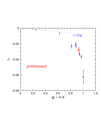
Figure 2: $c_{A}$ as a function of $g_{0}^{2}$. The dotted line is 1-loop PT.

where $Z_{q}$ is the quark wave function RC. In (9) four $Z_{q}^{-1/2}$ factors appear, because the $\Lambda$’s are four-leg amputated amplitudes. In Fig. 2 of [8] the results of a number of Monte Carlo measurements of the $\langle\bar{K}_{0}|\widehat{O}^{\Delta S=2}|K\rangle$ amplitude are shown as a function of $m_{K}^{2}$ [7]. It is clearly seen that the long sought chiral behaviour of $\langle\bar{K}_{0}|\widehat{O}^{\Delta S=2}|K\rangle$ is correctly reproduced when the NP renormalization procedure described in this section is employed, in conjunction with the SW-Clover-Leaf improved fermionic action [9] [10]. Similarly good results have also been reported by the JLQCD collaboration in the case of the standard Wilson action [11].

A possible difficulty with the idea of extracting the NP values of RC&MC’s from quark/gluon matrix elements is that a lattice gauge fixing is required in the simulations, leaving behind the problem of Gribov ambiguities.

The next obvious step within this approach is to go over to the much more complicated and interesting case of the $\Delta I=1/2$ ENLWH, where the problem of the subtraction of lower dimensional operators with power divergent MC’s has up to now forbidden a reliable computation of the $K\rightarrow\pi\pi|_{\Delta I=1/2}$ amplitude [12] [13]. The two operators relevant in this case belong to the [$8,1$] representation of the chiral group. They are usually indicated by $O^{(\pm)}$ and their bare expression is

$$\begin{array}[]{l}O^{(-)}_{0}=[(\bar{s}\gamma^{L}_{\mu}d)(\bar{u}\gamma^{L}_{\mu}u)-(\bar{s}\gamma^{L}_{\mu}u)(\bar{u}\gamma^{L}_{\mu}d)]-\\ -[u\leftrightarrow c]\\ O^{(+)}_{0}={1\over 5}[(\bar{s}\gamma^{L}_{\mu}d)(\bar{u}\gamma^{L}_{\mu}u)+(\bar{s}\gamma^{L}_{\mu}u)(\bar{u}\gamma^{L}_{\mu}d)+\\ +2(\bar{s}\gamma^{L}_{\mu}d)(\bar{d}\gamma^{L}_{\mu}d)+2(\bar{s}\gamma^{L}_{\mu}d)(\bar{s}\gamma^{L}_{\mu}s)]-\\ -[(\bar{s}\gamma^{L}_{\mu}d)(\bar{c}\gamma^{L}_{\mu}c)+(\bar{s}\gamma^{L}_{\mu}c)(\bar{c}\gamma^{L}_{\mu}d)]\end{array}$$

As we repeatedly said, the explicit breaking of chiral symmetry due to the presence of the Wilson term in the action, induces the mixing of $O^{(\pm)}_{0}$ with operators belonging to chiral representations other than the $[{\mbox{\boldmath{$8,1$}}}]$. Taking into account the symmetries left unbroken by the lattice regularization, it is easily seen that the renormalized, finite lattice operators, which in the fully interacting theory will transform as an [$8,1$] representation, must have the expression

$$\begin{array}[]{l}\widehat{O}^{(\pm)}=Z^{(\pm)}[O^{(\pm)}_{0}+\sum_{i=1}^{4}Z^{(\pm)}_{i}O^{(\pm)}_{i}+\\ +Z_{5}^{S(\pm)}\bar{s}\sigma_{\mu\nu}F_{\mu\nu}d+Z_{5}^{P(\pm)}\bar{s}\sigma_{\mu\nu}\widetilde{F}_{\mu\nu}d+\\ +Z_{3}^{S(\pm)}\bar{s}d+Z_{3}^{P(\pm)}\bar{s}\gamma_{5}d]\end{array}$$ (10)

Let us in turn examine the various terms in (10).

$\bullet$ Dimension 6 operators

The spin and color structure of the operators of dimension 6 contributing here is obviously the same as the one of the $\Delta S=2$ case discussed before. Only the flavor structure is different.

$\bullet$ Dimension 5 operators

If the GIM mechanism is operative, the coefficients $Z_{5}^{S(\pm)}$ are actually finite, because the potential $1/a$ divergence is replaced by a $m_{c}-m_{u}$ factor. As for $Z_{5}^{P(\pm)}$, GIM and CPS symmetry [12] (CPS = CP $\times$ symmetry under $s\rightarrow d$ exchange) make it finite and vanishing in the limit of exact vector flavor symmetry (exact $SU(N_{f})_{V}$).

$\bullet$ Dimension 3 operators

The GIM mechanism softens the divergence of $Z_{3}^{S(\pm)}$, reducing it from $1/a^{3}$ to $(m_{c}-m_{u})/a^{2}$. As before, CPS symmetry makes $Z_{3}^{P(\pm)}$ vanishing in the limit of exact $SU(N_{f})_{V}$.

An important observation at this point is that the Maiani-Testa no-go theorem [14] (which states that in euclidean region essentially only matrix elements of operators between one-particle states can be extracted from Monte Carlo data) forces us to limit our considerations to the $\langle K|\widehat{O}^{(\pm)}|\pi\rangle$ matrix elements, leaving the reconstruction of the $K\rightarrow\pi\pi$ amplitude to the use of the SPT’s

$$\begin{array}[]{l}\langle 0|O^{\triangle S=1}_{[\mbox{\boldmath{$\scriptstyle{8,1}$}}]}|K^{0}\rangle=i2\,\alpha_{2}\,{m^{2}_{K}-m^{2}_{\pi}\over F_{\pi}}\\ \langle\pi^{+}(p)|O^{\triangle S=1}_{[\mbox{\boldmath{$\scriptstyle{8,1}$}}]}|K^{+}(q)\rangle=-2\,\alpha_{2}\,{m^{2}_{K}\over F_{\pi}^{2}}+4\alpha_{1}\,{(p\cdot q)\over F^{2}_{\pi}}\\ \langle\pi^{+}\pi^{-}|O^{\triangle S=1}_{[\mbox{\boldmath{$\scriptstyle{8,1}$}}]}|K^{0}\rangle=i4\,\alpha_{1}\,{m^{2}_{K}-m^{2}_{\pi}\over F_{\pi}^{3}}\end{array}$$

valid for an [$8,1$] $\Delta S=1$ chiral operator. From the above equations it is in fact immediately seen that the $K\rightarrow\pi\pi$ amplitude can be obtained from the slope of $\langle\pi^{+}(p)|O^{\triangle S=1}_{[\mbox{\boldmath{$\scriptstyle{8,1}$}}]}|K^{+}(q)\rangle$ as a function of $(p\cdot q)$. Notice that, proceeding in this way, only the MC’s of the parity-conserving operators contributing to (10) will be necessary.

Let me now briefly illustrate the strategy for the construction of the $\Delta I=1/2$ ENLWH (see also [8]). The method we propose to arrive at a NP evaluation of the finite and power-divergent MC’s in (10) is a generalization of the approach described before to deal with the case of $\widehat{O}^{\Delta S=2}$.

To avoid uncontrollable numerical instabilities when the simultaneous computation of finite and infinite (in the limit $a\rightarrow 0$) MC’s from a single (large) set of linear equations is attempted, it is more convenient to separate the subtraction of power divergences from the subsequent finite mixing. We thus subdivide the whole procedure in two steps.

$\bullet$ One first defines the “intermediate” (power divergent) mixing constants, $C_{5}^{(\bar{s}d)}$ and $C_{i}^{(\bar{s}d)(\pm)}$, by requiring

$$\begin{array}[]{l}\mbox{Tr}(\hat{\mbox{I}\!\!\mbox{P}}_{\bar{s}d}\Lambda^{(\pm)}_{6,i}(\bar{q}q;\mu))=0,\ i=0,1,\ldots,4\\ \mbox{Tr}(\hat{\mbox{I}\!\!\mbox{P}}_{\bar{s}d}\Lambda_{5}(\bar{q}q;\mu))=0\end{array}$$ (11)

where $\hat{\mbox{I}\!\!\mbox{P}}_{\bar{s}d}$ is the projector over the color and spin structure of the operator $\bar{s}d$ and the amplitudes $\Lambda^{(\pm)}_{6,i}(\bar{q}q;\mu)$ and $\Lambda_{5}(\bar{q}q;\mu)$ are respectively the amputated $\bar{q},q$ matrix elements of the operators

$$\begin{array}[]{l}O^{(\pm)}_{6,i}=O^{(\pm)}_{i}+C_{i}^{(\bar{s}d)(\pm)}\bar{s}d,\,\,i=0,1,...,4\\ O_{5}=\bar{s}\sigma_{\mu\nu}F_{\mu\nu}d+C_{5}^{(\bar{s}d)}\bar{s}d\end{array}$$

$\bullet$ The second step consists in determining the finite MC’s, $Z^{(\pm)}_{i}$ and $Z^{(\pm)}_{5}$, by imposing the (non-homogeneous) set of linear conditions

$$\begin{array}[]{l}\mbox{Tr}(\hat{\mbox{I}\!\!\mbox{P}}_{5}\widetilde{\Lambda}^{(\pm)}_{PC}(\bar{q}gq;\mu))=0\\ \mbox{Tr}(\hat{\mbox{I}\!\!\mbox{P}}_{i}\widetilde{\Lambda}^{(\pm)}_{PC}(\bar{q}q\bar{q}q;\mu))=0,\ i=1,\ldots,4\end{array}$$

where the amplitudes $\widetilde{\Lambda}^{(\pm)}_{PC}$ are the appropriately amputated matrix elements of the (by now only logarithmically divergent) parity-conserving part of the operator (10), i.e. of the operator

$$\widetilde{O}_{PC}^{(\pm)}=\Big{[}O^{(\pm)}_{0}+\sum_{i=1}^{4}Z^{(\pm)}_{i}O^{(\pm)}_{6,i}\Big{]}_{PC}+Z^{S(\pm)}_{5}O_{5}$$

A feasibility study of the procedure outlined above is under way [15].

4 Schrödinger Functional

The functional integral with Dirichlet boundary conditions along the time direction

$${\cal{K}}(\Phi_{2},\Phi_{1};T)=\int_{\Phi_{1}(\vec{x})=\Phi(\vec{x},0)}^{\Phi_{2}(\vec{x})=\Phi(\vec{x},T)}{\cal{D}}\mu[\Phi]e^{-S[\Phi]}$$ (12)

yields the amplitude to find the field configuration $\Phi_{2}=\Phi_{2}(\vec{x})$ at time $t=T$, if the field configuration was $\Phi_{1}=\Phi_{1}(\vec{x})$ at time $t=0$. It thus represents the matrix element of the (Euclidean) transfer matrix, $e^{-HT}$, between the Schrödinger states $|\Phi_{2}\rangle$ and $|\Phi_{1}\rangle$:

$${\cal{K}}(\Phi_{2},\Phi_{1};T)=\langle\Phi_{2}|e^{-HT}|\Phi_{1}\rangle$$ (13)

More generally, given the functionals

$$Q_{k}(x_{k})=Q_{k}[\Phi(\vec{x}_{k},t_{k}),\delta/\delta\Phi(\vec{x}_{k},t_{k})],\,k=1,...,n$$

one can compute the expectation values

$$\begin{array}[]{l}\langle Q_{1}(x_{1})Q_{2}(x_{2})...Q_{n}(x_{n})\rangle\equiv\\ \\ \equiv\int_{\Phi_{1}}^{\Phi_{2}}{\cal{D}}\mu[\Phi]e^{-S[\Phi]}Q_{1}(x_{1})Q_{2}(x_{2})...Q_{n}(x_{n})=\\ \\ =\langle\Phi_{2}|e^{-HT}\prod_{k=1}^{n}e^{Ht_{k}}Q_{k}(x_{k})e^{-Ht_{k}}|\Phi_{1}\rangle\end{array}$$

In QCD one must take $\Phi_{2}=\{\vec{A}_{2},\bar{\psi}_{2}^{(+)},\psi_{2}^{(-)}\}$ and $\Phi_{1}=\{\vec{A}_{1},\bar{\psi}_{1}^{(-)},\psi_{1}^{(+)}\}$, where the superscripts $(\pm)$ appended to the $\bar{\psi},\psi$ fields are there to remember us that only half of the fermionic components can be assigned at each time boundary [16].

The YM and the QCD SF’s have been formally constructed in the continuum, in the temporal gauge ($A_{0}=0$), in [17] and in [18] respectively. In [18] the superscripts $(\pm)$ were taken with reference to the positive and negative frequency decomposition of the fermionic fields, as this is the most suitable choice when working in the temporal gauge. The corresponding constructions on the lattice, where no gauge fixing is necessary, were carried out in [19] and in [20]. In the QCD case Dirichlet boundary conditions on the spin projections

$$\begin{array}[]{l}\psi^{(\pm)}=\frac{1\pm\gamma_{0}}{2}\psi,\quad\bar{\psi}^{(\pm)}=\bar{\psi}\frac{1\pm\gamma_{0}}{2}\end{array}$$

were imposed [20]. Studies of the renormalization properties of the lattice QCD SF can be found in [21] and in [22].

In absence of fermions, the SF formalism was implemented in lattice simulations to study the running of the gauge coupling. A renormalized coupling, $\alpha_{s}$, as a function of $q=1/L$ ($L^{d}=$ lattice volume) is defined by looking at the response of $\cal K$ under small changes of an externally applied color-magnetic field [23]. The running of $\alpha_{s}$ with $1/L$ is extracted in a recursive way, in a two step procedure [24].

$\bullet$ Starting with a given (small) value of $g_{0}^{2}$, the variation of $\alpha_{s}$, $\Delta\alpha_{s}^{(1)}=\alpha_{s}(L)-\alpha_{s}(L_{1}=sL)$, ensuing from an increase of the number of lattice points by a factor $s^{d}$ ($L=Na\rightarrow L_{1}=sNa$), is computed and its continuum limit is extrapolated from data taken at decreasing values of $a/L$ with fixed $\alpha_{s}(L)$.

$\bullet$ Then the physical value of the lattice spacing is increased, at fixed renormalized coupling (by adjusting the bare coupling $g_{0}^{2}$), in order to have, with a number of points equal to the initial one, a renormalized coupling precisely equal to $\alpha_{s}(L_{1})$, to be in position to start a second iteration.

At this point the whole procedure is repeated, by measuring the variation $\Delta\alpha_{s}^{(2)}=\alpha_{s}(L_{1})-\alpha_{s}(L_{2}=sL_{1})$ for an increase of the number of lattice points again by a factor $s^{d}$. At each step the limit $a/L\rightarrow 0$ of the variations $\Delta\alpha_{s}^{(i)}$ is appropriately taken.

The results obtained with this method are very accurate (few % errors) and compare very nicely [25] with the results of [26], derived employing a similar iterative procedure, but using for the renormalized gauge coupling a definition given in terms of ratios of twisted Polyakov loops. For a measure of the running of $\alpha_{s}$ defined directly from the three-gluon vertex, see [27].

The introduction of fermions in the SF opens the way to a wealth of very accurate NP measurements of RC&MC’s which ultimately will allow the (on-shell) construction of the fully O($a$) improved QCD lattice theory. The use of the SF approach has the further noticeable advantages of providing a formalism which allows to perform Monte Carlo simulations

$\bullet$ directly at the chiral point, $M_{0}=M_{cr}$,

$\bullet$ with no need of fixing the gauge.

Up to now the method has been used to construct (in the quenched approximation) the O($a$) improved QCD action and the correspondingly improved bilinear quark operators. However, the approach seems to be sufficiently general to be capable to encompass the much more complicated and interesting case of the four-quark operators.

The general idea is to start with the SW nearest-neighbor improved fermion action

$$S_{{}_{SW}}=S_{{}_{W}}+a^{5}\frac{i}{4}c_{{}_{SW}}\sum_{x}\bar{\psi}(x)\sigma_{\mu\nu}P_{\mu\nu}(x)\psi(x)$$ (14)

where $S_{{}_{W}}$ is the standard Wilson action (from now on $r=1$) and $P_{\mu\nu}$ is any lattice discretization of the gauge field strength [28], and to determine the value of $c_{{}_{SW}}$ and of all the necessary RC&MC’s, by requiring that on-shell chiral WTI’s involving quark bilinear do not have O($a$) corrections. The “tree level” improvement of the Wilson action (eq. (14) with $c_{{}_{SW}}=1$) kills in on-shell Green functions all terms that in PT are of O($a\,(g_{0}^{2}\log a)^{n}$) (i.e. the terms that in the continuum limit, $g_{0}^{2}\sim 1/\log a$, are effectively of order $a$), leaving uncancelled O($a$) subleading logarithmic corrections [10].

To illustrate the SF method let me describe the strategy for the determination of quantities like $c_{{}_{SW}}$, $Z_{A}$, $Z_{V}$ or the critical mass, $M_{cr}$, which are only functions of $g_{0}^{2}$. More subtle is the problem of computing the renormalized coupling constant, $g_{R}^{2}$, or the renormalized quark mass, $m_{R}$, or certain MC’s, because it turns out that the general mass-independent renormalization scheme, consistent with O($a$) improvement, requires a rescaling of the bare parameters by mass dependent factors [22].

The crucial observation which makes the whole program actually feasible is that, for the sake of computing the functional dependence of $c_{{}_{SW}}$, $Z_{A}$, $Z_{V}$, or $M_{cr}$, on $g_{0}^{2}$, for small $g_{0}^{2}$, all the necessary numerical simulations can be quite happily performed deep in the perturbative region. This can be realized by working in a not too large volume in order to keep lattice momenta, $p_{n}=\frac{2\pi}{L}n$, much larger than the typical mass scale of the theory. Indicatively, if $N$ is the number of points per lattice side, one should have

$$2\pi/L\gg\Lambda_{QCD}\,\,\mbox{i.e.}\,\,N\ll\exp(1/2b_{0}g_{0}^{2})$$

At the same time to keep under control discretization effects, which scale like powers of $a/L$ (times possible logarithmic factors), one must also require

$$L/a=N\sim\mbox{large}$$

With the choices $g_{0}^{2}<1$ and $N\mathrel{\hbox to0.0pt{\lower 3.0pt\hbox{$\mathchar 536\relax$}\hss}\raise 2.0pt\hbox{$\mathchar 318\relax$}}10$ both conditions are well satisfied and the physical volume of the box (determined, for instance, as explained in [23]) turns out to be rather small ($L\simeq 0.5$ fm). An important consequence of these choices is that simulations can be performed directly at the critical mass, $M_{0}=M_{cr}$, as for small $g_{0}^{2}$ the lowest eigenvalue of the Dirac operator is O($1/L$) and not O($M_{0}-M_{cr}$).

Figure 1: $c_{{}_{SW}}$ for large and small $g_{0}^{2}$. Comparison with 1-loop TIPT (crosses) and PT (dots) is shown. The solid line is a numerical interpolation of the data.

To illustrate the method in a concrete way, let me discuss the determination of $c_{{}_{SW}}(g_{0}^{2})$ and $M_{cr}(g_{0}^{2})$. One starts from the lattice PCAC equation

$$\langle\partial_{\mu}A_{\mu}^{f}(\vec{x},x_{0})O^{f}\rangle=2m\langle P^{f}(\vec{x},x_{0})O^{f}\rangle+\mbox{O}(a)$$ (15)

where ($x\notin\mbox{Support of}$ $O^{f}$)

$$A_{\mu}^{f}=\bar{\psi}\gamma_{\mu}\gamma_{5}\frac{\tau^{f}}{2}\psi,\,\,P^{f}=\bar{\psi}\gamma_{5}\frac{\tau^{f}}{2}\psi$$

$O^{f}$ is an operator which creates a pseudoscalar state at $t=0$. Explicitly one can take

$$O^{f}=-\int_{0}^{L}d^{3}y\int_{0}^{L}d^{3}z\frac{\delta}{\delta\psi_{1}^{(+)}(\vec{y})}\gamma_{5}\frac{\tau^{f}}{2}\frac{\delta}{\delta\bar{\psi}_{1}^{(-)}(\vec{z})}$$

In (15) it is understood that the fermionic boundary values are set to zero after the action of the grassmannian functional derivatives. A plot of

$$R_{A}=\langle\partial_{\mu}A_{\mu}^{f}(\vec{x},x_{0})O^{f}\rangle/\langle P^{f}(\vec{x},x_{0})O^{f}\rangle$$

as a function of the current insertion time, $x_{0}/a$, shows strong violations of chirality [29], when the standard Wilson action is employed. These effects are to be attributed to the (large) O($a$) corrections affecting eq. (15). They can be eliminted from all Green functions at unequal points, following the steps described below

$\bullet$ add the SW-term, $\frac{i}{4}c_{{}_{SW}}a^{5}\sum_{x}\bar{\psi}\sigma_{\mu\nu}P_{\mu\nu}\psi$, to the standard Wilson action,

$\bullet$ construct renormalized improved quark operators, $\widehat{O}^{I}_{q}$, by adding to their bare expression, $O_{q}$, a suitable linear combination of operators, $O^{(i)}_{q}$, with dimensions up to $\mbox{dim}O_{q}^{(i)}=\mbox{dim}O_{q}+1$,

$\bullet$ fix, at any given value of $g_{0}^{2}$, $c_{{}_{SW}}$ and the corresponding MC’s by requiring O($a$) corrections to be absent from WTI’s.

The renormalized, O($a$)-improved expressions of the axial current and of the pseudoscalar density are ($m_{q}\equiv M_{0}-M_{cr}$)

$$\begin{array}[]{l}\widehat{A}_{\mu}^{fI}=Z_{A}[(1+am_{q}b_{A})A_{\mu}^{f}+ac_{A}\partial_{\mu}P^{f}]\\ \widehat{P}^{fI}=Z_{P}(1+am_{q}b_{P})P^{f}\end{array}$$ (16)

where at tree level, beside $c_{{}_{SW}}^{tree}=1$, one has $b_{A}^{tree}=b_{P}^{tree}=1$, $c_{A}^{tree}=0$ [10]. At any given $g_{0}^{2}$ the improved ratio

$$\widehat{R}^{I}_{A}=\langle\partial_{\mu}\widehat{A}_{\mu}^{aI}(\vec{x},x_{0})O^{f}\rangle/\langle\widehat{P}^{aI}(\vec{x},x_{0})O^{f}\rangle$$

is measured for different values of $x_{0}/a$ and for two different (zero and non-zero) boundary gauge field configurations. Actually to the order one is working (terms O($a^{2}$) are neglected), the behavior of $\widehat{R}^{I}_{A}$ as a function of $x_{0}/a$ is only sensitive to $c_{{}_{SW}}$ and $c_{A}$. In fact one can write

$$\begin{array}[]{l}\widehat{R}^{I}_{A}=\frac{Z_{A}}{Z_{P}}\frac{1+am_{q}b_{A}}{1+am_{q}b_{P}}\frac{\langle(\partial_{\mu}A_{\mu}^{f}+ac_{A}\partial^{2}P^{f})O^{f}\rangle}{\langle P^{f}O^{f}\rangle}+\mbox{O}(a^{2})\end{array}$$

The nice results obtained for $c_{{}_{SW}}(g_{0}^{2})$ and $c_{A}(g_{0}^{2})$ by imposing that $\widehat{R}^{I}_{A}$ is independent of i) $x_{0}/a$, ii) the particular form of the operator $O^{f}$ iii) the boundary values of the gauge fields, are shown in Figs. 1 and 2. While $c_{A}$ is negligible to all practical extents, $c_{{}_{SW}}$ appears to be a rapidly increasing function of $g_{0}^{2}$. Data for $c_{{}_{SW}}$ are larger than expected from simple “tadpole improvement” arguments [30].

Once $c_{{}_{SW}}$ and $c_{A}$ have been fixed, by varying $M_{0}$, one can determine $M_{cr}$ as the value of $M_{0}$ for which $R_{A}$ (and of course also $\widehat{R}^{I}_{A}$) vanishes. Data for $\kappa_{cr}$, measured at large and small $g_{0}^{2}$, are shown in Fig. 3, together with the results from 1-loop Tadpole Improved PT (TIPT) and from 1-loop straight PT, respectively.

Figure 3: $\kappa_{cr}$ for large and small $g_{0}^{2}$. Comparison with 1-loop TIPT (crosses) and PT (dots) is shown.

It is clearly seen that the non-monotonic behavior of $\kappa_{cr}$ is in striking contrast with tadpole improvement expectations. This is not surprising in view of the fact that a proper definition of $M_{cr}$ requires a linearly divergent subtraction.

Figure 4: $Z_{A}$ as a function of $g_{0}^{2}$. Comparison with 1-loop TIPT (crosses) and PT (dots) is shown.

Absence of O($a$) corrections in WTI’s is a strong requirement which also allows an accurate evaluation of the current RC’s. In Figs. 4 and 5 we show the results for $Z_{A}$ and $Z_{V}$, as functions of $g_{0}^{2}$, together with the predictions of 1-loop TIPT and PT. In both cases numbers from TIPT interpolate quite nicely Monte Carlo results. Perhaps the lesson we can draw from the different ability of TIPT in reproducing data directly extracted from simulations is that TIPT can be really useful only for estimating finite RC&MC’s.

We would like to conclude this section by stressing again that the use of the SF formalism in Monte Carlo simulations seems to be extremely promising and has already provided us with a lot of very accurate results. It would really be a great achievement if one could extend this approach to the construction of finite, renormalized four-quark operators.

5 NP renormalization by “heating - cooling” steps

For completeness, in this section I wish to discuss a completely different NP renormalization method based on “heating-cooling” Monte Carlo steps. The method is designed to deal with the problem of giving finite and renormalized field theoretical definitions of the topological charge density, $q(x)$ and of the topological susceptibility, $\chi$, in lattice gauge theories [31]. The method is not new, but is has been recently tested with success in certain exactly solvable $\sigma$-models [32] and, more interesting, it has revealed an unexpected vanishing of $\chi$ across the YM deconfining temperature [33].

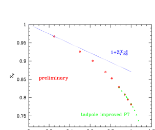
Figure 5: $Z_{V}$ as a function $g_{0}^{2}$. Comparison with 1-loop TIPT (triangles) and PT (dots) is shown.

The topological susceptibility has been the object of many theoretical and numerical investigations not only because it is directly related to the mass of the flavor singlet pseudoscalar meson ($m^{2}_{\eta_{S}}=\frac{2N_{f}}{F^{2}_{\pi}}\chi$) [34], but also because it is a natural question to ask whether and how it is possible to give on a lattice a notion which would reduce to the standard notion of topology in the continuum limit. For lack of space (see however [35] and references therein), I will not mention definitions of the topological charge, based on purely geometrical considerations (the first of which dates back to [36]), nor the construction of $\chi$, based on the use of the flavor singlet axial WTI [37]. These two topics are, anyway, outside the aim of this talk, as in both cases, by construction, no renormalization is expected to be necessary.

The formula for the topological charge in a continuum gauge theory (Pontrjagin number) is $Q=\int d^{4}xq_{c}(x)$, where $q_{c}(x)=\frac{g_{0}^{2}}{32\pi^{2}}\epsilon_{\mu\nu\rho\sigma}\mbox{Tr}(F_{\mu\nu}F_{\rho\sigma})$ is the topological charge density. On a lattice one can use the definition

$$q(x)=-\frac{1}{2^{4}32\pi^{2}}\sum_{\mu\nu\rho\sigma=\pm 1}^{\pm 4}\epsilon_{\mu\nu\rho\sigma}\mbox{Tr}(P_{\mu\nu}P_{\rho\sigma})$$

where $P_{\mu\nu}$ is a discretization of $F_{\mu\nu}$ [28]. It is, in fact, immediately seen that, in the naive $a\rightarrow 0$ limit, $q(x)\rightarrow a^{4}q_{c}(x)+\mbox{O}(a^{6})$. This means that in the continuum (field-theoretical) limit, $g_{0}^{2}\rightarrow 0$ with $g_{0}^{2}\sim 1/\log a$, we will have

$$q(x)\rightarrow Z_{Q}(g_{0}^{2})a^{4}(g_{0}^{2})q_{c}(x)+\mbox{O}(a^{6})$$ (17)

From the previous equations it naturally follows that the lattice version of the continuum topological susceptibility, $\chi_{c}=\int d^{4}x\langle T(q_{c}(x)q_{c}(0))\rangle$, can be taken to be

$$\chi=\sum_{x}\langle T(q(x)q(0))\rangle$$

According to the general rules of field theory, $\chi_{c}$ and $\chi$ will be related in the continuum limit by

$$\chi=Z_{Q}^{2}(g_{0}^{2})a^{4}(g_{0}^{2})\chi_{c}+C_{\chi}(g_{0}^{2})+\mbox{O}(a^{6})$$ (18)

The factor $Z_{Q}^{2}(g_{0}^{2})$ comes from (17), while the subtraction term, $C_{\chi}(g_{0}^{2})$, is a consequence of the mixing of $\chi$ with the operator $\mbox{Tr}(F_{\mu\nu}F_{\mu\nu})$ and the identity. A NP estimate of $Z_{Q}(g_{0}^{2})$ and $C_{\chi}(g_{0}^{2})$ relies on the simple observation that short range fluctuations (at the scale of the cut-off) are responsible for renormalization effects, while physical effects, like confinement, come from much larger distances (of the order of the correlation length, $\xi$). When approaching the continuum limit, the two scales are widely separated. Using a local Monte Carlo updating algorithm, fluctuations at distances $\sim a$ will be soon thermalized, whereas fluctuations at the scale of $\xi$ are critically slowed down.

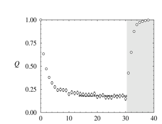
Figure 6: $Q$ as a function of the heating step, $n$.

For a standard local algorithm, like Metropolis, the time (# of sweeps) necessary to thermalize fluctuations at distances $d$ grow proportionally to $d^{z}$ with $z\sim 2$. Changes in the global (topological) properties of the gauge configuration are expected to require a much longer (exponential) time. To measure $Z_{Q}$ a gauge configuration with topological charge 1 is placed on the lattice and, at any given temperature, $\beta=2N_{c}/g_{0}^{2}$, it is progressively heated (only link-variable changes that make the action increase are accepted) for a few Monte Carlo sweeps. $Z_{Q}$ is the value at which $Q$, measured as a function of the Monte Carlo step, $n$, reaches a plateau (Fig. 6). Data have very small errors and $Z_{Q}$ can be extracted with remarkable accuracy. The last points of Fig. 6 (shaded area) are obtained by cooling back the configuration. It is seen that the initial value $Q=1$ is reobtained, thus showing that the global properties of the successive gauge configurations one has gone through were left unchanged by the heating process. Once $Z_{Q}$ is known, $C_{\chi}$ is determined starting from a (topologically) trivial gauge configuration and measuring $\chi$ for a few Monte Carlo steps, until it reaches a plateau (Fig. 7). Since in (18) the first term is zero ($Q=0$), the height of the plateau is precisely $C_{\chi}$. Cooling back the gauge configuration, one checks that no unwanted non-trivial contributions to $\chi$ have been introduced during the heating process.

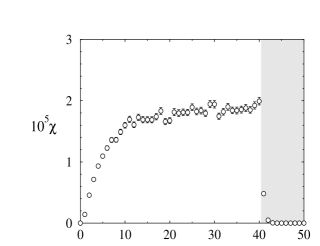
Figure 7: $\chi$ as a function of the heating step, $n$.

6 Short distance expansions, higher twists and condensates

Short Distance Expansions (SDE’s) are among the very few approaches, besides instanton calculus and SPT’s, that may provide pathways to NP analytical calculations in (non-supersymmetric) QCD. It is then of the utmost importance to understand to what extent corrections to the leading term of the expansion can be rigorously defined and reliably computed. The heart of the problem is that, while the calculation of Wilson coefficients is necessarily truncated to some finite order in $\alpha_{s}$, exponentially small ($\sim\exp(-c/\alpha_{s})$) non-perturbative corrections (as those given by next order terms) are retained.

The whole issue is complicated by the difficulties arising from the existence of renormalon ambiguities in the Borel resummation of PT. As is well known [39], perturbative series in field theories are only asymptotic and in the most interesting cases (gauge theories) are not Borel summable, as a consequence of the presence of singularities located on the positive real axis of the Borel $u$-plane. We recall that a pole at the position $u=u_{0}>0$ leads to an ambiguity of the kind $\exp(-\frac{c}{g_{0}^{2}}u_{0})$ in the Borel resummed series.

In all instances where a large scale expansion is performed ($e^{+}e^{-}$-annihilation, DIS scattering, Heavy Quark Effective Theory (HQET),…), further renormalon singularities appear. As in the full theory, they come from the factorial growth of the weight of certain classes of diagrams when the running coupling $g^{2}(k)$ ($k$ is the loop momentum) is expanded as a power series in $g^{2}(\mu)$ ($\mu$ is some fixed renormalization scale) . The situation can be summarized as follows.

$\bullet$ Borel poles coming from the loop integration region where $-b_{0}\log(k/\mu)>0$, i.e. where $k<\mu$ ($b_{0}>0$ in our conventions), are called Infra-Red (IR) renormalons and affect Wilson coefficients.

$\bullet$ Poles coming from the loop integration region where $-b_{0}\log(k/\mu)<0$, i.e. where $k>\mu$, are called Ultra-Violet (UV) renormalons. They show up in the hadronic matrix elements of the Wilson operators.

A lot of interesting work has been recently done (for a nice review see [40]) on the question of the appearance and cancellation of renormalon ambiguities. By matching the Wilson expansion against full theory calculations, it was shown that SDE-renormalon ambiguities must cancel between Wilson coefficients and hadronic matrix elements. The way it happens is rather involved and the details depend on whether one uses a soft (e.g. dimensional) or a hard (e.g. lattice) regularization.

In spite of this nice result, it has been argued in [41] that a further strong assumption on the relative magnitude of perturbative corrections vs NP terms is necessary and unavoidable, if one wants to give a precise meaning to large scale expansions beyond the leading term. To illustrate the point I will closely follow ref. [41].

Let ${\cal{P}}_{fi}(Q^{2})\equiv\langle f|\widehat{P}(Q^{2})|i\rangle$ be the Fourier transform of some bilocal T-product of operators. The expansion of ${\cal{P}}_{fi}(Q^{2})$ for large $Q^{2}$ has the form

$$\begin{array}[]{l}{\cal{P}}_{fi}(Q^{2})=C_{1}(\frac{Q^{2}}{\mu^{2}})\langle f|O_{1}(\mu)|i\rangle+\\ +\frac{1}{(Q^{2})^{n}}\,C_{2}(\frac{Q^{2}}{\mu^{2}})\langle f|O_{2}(\mu)|i\rangle\end{array}$$ (19)

where $O_{1}(\mu)$ and $O_{2}(\mu)$ are local operators normalized at scale $\mu$, with $\mbox{dim}O_{2}=\mbox{dim}O_{1}+2n$. For simplicity only two terms have been included in (19), but the argument can be readily extended to any number of terms. The operator $\widehat{P}$ is renormalized (in the full theory) at a scale $M$ and the dependence of $C_{1}$ and $C_{2}$ on $M$ is understood. The usefulness of the expansion (19) lies in the fact that short distance NP effects are contained in the matrix elements of the operators $O_{i}$, while the $C_{i}$ can be reliably computed in PT at large $\mu$. It is assumed that the matrix element of $O_{1}$ is exactly known, either because it is the identity or because it is a conserved operator. The question is whether one can unambiguously define $O_{2}$ by matching the large $Q^{2}$ (perturbative) computation of the rhs of (19) in the full theory with the form of the expansion in the lhs. Barring exceptional cases, the interesting situation is when $O_{2}$ mixes with $O_{1}$.

If dimensional regularization is used, IR renormalon singularities will appear in the Borel transform of $C_{1}$, making its perturbative series non-Borel summable. Matching implies that a compensating UV renormalon ambiguity will affect the matrix elements of $O_{2}$. This simple argument already shows where the heart of the problem with the definition of higher twist operators (such as $O_{2}$) lies: the perturbative series for the Wilson coefficients have renormalon ambiguities that are of the same (exponentially small) magnitude of the NP effects described by the higher dimensional terms one is including in the Wilson expansion.

One might imagine to overcome this difficulty by alternatively trying to define higher order terms in SDE’s by either comparing different expansions involving the same higher dimensional operators (at the expenses of a certain number of predictions) or by resorting to a NP, say lattice, determination of the matrix elements of the relevant higher twist operators. It turns out [41] that the two methods are equivalent and offer only a partial solution of the problem, in the sense that

1) - after renormalizing $O_{2}$, $C_{1}$ is free of the leading renormalon ambiguity of order $\frac{1}{(Q^{2})^{n}}\sim\exp(-\frac{4\pi}{b_{0}\alpha_{s}(Q^{2})}2n)$.

2) - Extra renormalon poles, located further away along the positive real Borel axis are assumed to be related to the presence of even higher dimensional operators in (19) and could be in turn eliminated by sacrificing extra physical predictions to fix their ambiguous matrix elements.

3) - However, since the Wilson coefficients can only be known up to a certain order in PT (say, up to order $(\alpha_{s})^{k}$) and the cancellation of the leading renormalon starts to be numerically effective at some large order in PT (the higher the dimension of the involved operators, the larger the order the cancellations start to be operative), we must require higher order perturbative contributions to be negligible with respect to the exponentially small terms we are retaining in the expansion.

In formulae this means that for the expansion (19) to be useful the inequality

$$\begin{array}[]{l}(\alpha_{s}(Q^{2}))^{k+1}\mathrel{\hbox to0.0pt{\lower 3.0pt\hbox{$\mathchar 536\relax$}\hss}\raise 2.0pt\hbox{$\mathchar 316\relax$}}\exp[-\frac{4\pi|\mbox{dim}O_{2}-\mbox{dim}O_{1}|}{b_{0}\alpha_{s}(Q^{2})}]\end{array}$$ (20)

must hold . Unfortunately, whether or not inequalities like (20) are numerically satisfied in real life cannot be decided a priori.

The situation is even more troublesome in the case of “condensates”, i.e. when one is dealing with the vacuum expectation value (v.e.v.) of the T-product of, say, two currents, like in $e^{+}e^{-}$-annihilation. The v.e.v’s of the local operators appearing in the SDE are the NP quantities one would like to define properly and utilize to make predictions in other physical processes. Naively, i.e. according to what we were taught in our graduate courses in field theory, when a local operator, $O$, can mix with the identity, its v.e.v. will be power divergent and should be subtracted out. Furthermore, whatever the subtraction prescription is, physical results should not depend on it. Thus without loss of generality, one can always use the prescription $\widetilde{O}=O-\langle O\rangle\mbox{1$\!\!$I}$. The consequence of this argument is that the v.e.v. of a local operator cannot have a physical meaning. The only exception is when the v.e.v. in question plays the role of order parameter of some symmetry. The most obvious example of this situation is $\langle\bar{\psi}\psi\rangle$, which is the order parameter of chiral symmetry. In this case one can use the WTI of the chiral symmetry to define what is to be meant by $\langle\bar{\psi}\psi\rangle$ and, if required, to relate its value to the mass of the Goldstone boson, when $m_{q}\neq 0$.

This situation should be contrasted with the case of the condensate $F^{2}\equiv\langle\mbox{Tr}(F_{\mu\nu}F_{\mu\nu})\rangle$. $F^{2}$ is not the order parameter of any symmetry and, in fact, it does not appear in any useful WTI. Besides, if we recall that the v.e.v. of the trace of the energy-momentum density tensor, $\langle\theta_{\mu\mu}\rangle$, is proportional to $F^{2}$, we would be very strongly tempted to conclude that $F^{2}=0$, to prevent the vacuum to have infinite total energy. The last statement follows from the observation that Lorentz invariance implies $\langle\theta_{\mu\nu}\rangle=kg_{\mu\nu}$, so that vacuum energy finiteness requires $\langle\theta_{00}\rangle=0$, leading to the conclusion $k=0$ and hence $F^{2}=0$.

Acknowledgments

I would like to thank all my collaborators for innumerable conversations. My special thanks go to S. Capitani, M. Lüscher, G. Martinelli, A. Pelissetto, R. Petronzio, C. T. Sachrajda, R. Sommer, M. Talevi, M. Testa, A. Vladikas. I should also thank R. Sommer and H. Wittig for sending me Figs. 1 to 5 prior to publication.

References

- [1] K.G. Wilson, Phys. Rev. D10 (1974) 2445 and in “New Phenomena in Subnuclear Physics”, A. Zichichi ed. (Plenum, 1977).
- [2] L.H. Karsten and J. Smit, Nucl. Phys. B183 (1981) 103.
- [3] M. Bochicchio, L. Maiani, G. Martinelli, G.C. Rossi and M. Testa, Nucl. Phys. B262 (1985) 331.
- [4] L. Maiani and G. Martinelli, Phys. Lett. 178B (1986) 265.
-
[5]
G. Martinelli, Phys. Lett. 141B (1984) 395;
C. Bernad, A. Soni and T. Draper, Phys. Rev. D3 (1987) 3224. - [6] G. Martinelli, C. Pittori, C.T. Sachrajda, M. Testa and A. Vladikas, Nucl. Phys. B445 (1995) 81.
- [7] A. Donini, G. Martinelli, C.T. Sachrajda, M. Talevi and A. Vladikas, Phys. Lett. 360B (1995) 83 and in preparation.
- [8] M. Talevi, these proceedings.
- [9] B. Sheikholeslami and R. Wohlert, Nucl. Phys. B259 (1985) 572.
- [10] G. Heatlie, G. Martinelli, C. Pittori, G.C. Rossi and C.T. Sachrajda, Nucl. Phys. B352 (1992) 266.
- [11] Y. Kuramashi, these proceedings.
- [12] C. Bernard, T. Draper, G. Hockney and A. Soni, Nucl. Phys B (Proc. Supp.) 4 (1988) 483.
- [13] M.B. Gavela, L. Maiani, G. Martinelli, O. Pène and S. Petrarca, Phys. Lett. 211B (1988) 139.
- [14] L. Maiani and M. Testa, Phys. Lett. 245B (1990) 585.
- [15] G. Martinelli, G.C. Rossi, M. Talevi, M. Testa and A. Vladikas, in preparation.
-
[16]
F.D. Faddeev, in “Methods in Field Theory”, Les Houches, 1985,
R. Balian and J. Zinn-Justin eds. (North Hollond, 1986);
G. Immirzi, Z. Phys. C44 (1989) 655. - [17] G.C. Rossi and M. Testa, Nucl. Phys. B163 (1980) 109; Nucl. Phys. B176 (1980) 477; Nucl. Phys. B237 (1984) 442.
- [18] J.P. Leroy, J. Micheli, G.C. Rossi and K. Yoshida, Z. Phys. C48 (1990) 653.
- [19] M. Lüscher, R. Narayanan, P. Weisz and U. Wolff, Nucl. Phys. B384 (1992) 168.
- [20] S. Sint, Nucl. Phys. B421 (1994) 135.
- [21] S. Sint, Nucl. Phys. B451 (1995) 416.
- [22] M. Lüscher, S. Sint, R. Sommer and P. Weisz, hep-lat/9605038.
- [23] M. Lüscher, R. Sommer, P. Weisz and U. Wolff, Nucl. Phys. B389 (1993) 247; Nucl. Phys. B413 (1994) 481.
-
[24]
M. Lüscher, P. Weisz and U. Wolff, Nucl. Phys. B359 (1991) 221;
S. Caracciolo, R.G. Edwards. A. Pelissetto and A.D. Sokal, Phys. Lett. 75B (1995) 1891. - [25] G. de Divitiis, R. Frezzotti, M. Guagnelli, M. Lüscher, R. Petronzio, R. Sommer, P. Weisz and U. Wolff, Nucl. Phys. B437 (1995) 447.
- [26] G. de Divitiis, R. Frezzotti, M. Guagnelli and R. Petronzio, Nucl. Phys. B422 (1994) 382; Nucl. Phys. B433 (1995) 390.
- [27] B. Allés, D. Henty, H. Panagopoulos, C. Parrinello and C. Pittori, hep-lat/9605033.
-
[28]
M. Baake, B. Gemünden and R. Oendigen, J. Math. Phys. 23 (1982)
944;
J.E. Mandula, G. Zweig and J. Govaerts, Nucl. Phys. B228 (1983) 91 and 109. - [29] K. Jansen, C. Liu, M. Lüscher, H. Simma, S. Sint, R. Sommer, P. Weisz and U. Wolff, hep-lat/9512009.
- [30] G.P. Lepage and P.B. Mackenzie, Phys. Rev. D48 (1993) 2250.
- [31] B. Allés, M. Campostrini, A. di Giacomo, Y. Gündüc and E. Vicari, Phys. Rev. D48 (1993) 2284 and Nucl. Phys B (Proc. Supp.) 34 (1994) 504.
- [32] B. Allés, M. Beccaria and F. Farchioni, Phys. Rev. D54 (1996) 1044.
- [33] B. Allés, M. D’Elia and A. di Giacomo, hep-lat 9605013.
-
[34]
E. Witten, Nucl. Phys. B156 (1979) 269;
G. Veneziano, Nucl. Phys. B159 (1979) 213. -
[35]
M. Garcia Perez, these proceedings;
P. Hernandez, these proceedings. - [36] M. Lüscher, C.M.P. 85 (1982) 29.
- [37] M. Bochicchio, G.C. Rossi, M. Testa and K. Yoshida, Phys. Lett. 149B (1984) 487.
- [38] A. Di Giacomo, these proceedings.
-
[39]
G. ’t Hooft in “The whys of Subnuclear Physics”, A. Zichichi ed.
(Plenum, 1979);
B. Lautrup, Phys, Lett. 69B (1977) 943;
G. Parisi, Phys. Lett. 76B (1978) 65 and Nucl. Phys. B150 (1979) 163. - [40] C.T. Sachrajda, Nucl. Phys B (Proc. Supp.) 47 (1996) 100 and references therein.
- [41] G. Martinelli and C.T. Sachrajda, hep-ph 9605336.