UNIGRAZ- UTP- 17-09-96 Classical ${\rm U}(1)$ Lattice Gauge Theory in $D=2$

Abstract

Under the hypothesis of no topological structure below a certain scale, we prove that any ${\rm U}(1)$ lattice configuration corresponds to a classical ${\rm U}(1)$ gauge field with zero local field strength; i.e. any local representative of the pullback connection one-form is a pure gauge and the local curvature two-form is thus identical zero. The topological information is completely carried by the chart transitions. To each such ${\rm U}(1)$ lattice configuration we assign a Chern number, which generally depends on the reconstruction of the bundle and is only unique under certain restrictions.

1 Motivation

There is a recent increased interest in $QED_{2}$. This concerns the continuum as well as the lattice version of the model (c.f. [1] - [11]). The one flavor massless continuum model [12, 13] is analytically solvable and has been studied extensively. The reason for the increased interest is that $QED_{2}$ shows $QCD_{4}$ like behavior. This applies especially to the multi flavor situation [3]. The Maxwell equations for two dimensional electrodynamics also have topologically non trivial $C^{\infty}$ solutions with finite action which can be classified by their Chern number. These topological objects called instantons are considerably simpler to imagine for ${\rm U}(1)$ in $D=2$ than for $SU(2)$ in $D=4$ which is an additional appeal to study $QED_{2}$. Therefore one finds in $QED_{2}$ three closely related problems. There is the problem of the $\theta$-vacua, which naively speaking are superpositions of all topological sectors corresponding to different Chern numbers. Also observed in both models is the occurrence of the ${\rm U}_{A}(1)$ problem [14, 15]. $QED_{2}$ further allows for a Witten-Veneziano type formula [16, 17, 3].

It is not clear how important these topological nontrivial configurations are indeed for quantum physics. Naively such $C^{\infty}\in\cal{S}^{\ast}$ solutions should not contribute in the functional integration since the subset of such smooth solutions is of measure zero for the measure over $\cal{S}^{\ast}$. Nevertheless the topological susceptibility, which is the first Chern character for $QED_{2}$ vice versa the second Chern character for $QCD_{4}$, appears in the ${\rm U}_{A}(1)$ anomaly.

The lattice situation is quite different. First of all the lattice regularized version is analytically not solvable. Further assuming that the lattice model approximates in a certain limit the continuum model and thus also contributions from topology it is a priori not clear what differential geometry means for a set of points. Any straightforward bundle reconstruction will only lead to trivial bundles with Chern number zero. One way out is to provide the lattice with a very special topology and construct partially ordered sets which allow for non trivial bundles [18]. $QED_{2}$ can be also defined on a fuzzy sphere which allows a topological classification in a surprisingly intuitive way via the Hopf fibration [19, 20]. A third possibility is to regard the lattice as a directed complex with a certain realization like ${\rm T}^{2}$. This idea was pioneered by Lüscher [21] for $SU(2)$ in $D=4$ and put on a more axiomatic approach in [22] for ${\rm U}(1)$ in $D=2$.

Without the explicit construction of bundles the $\theta$-vacuum problem and the topological charge problem on the lattice could also be addressed by possible remnants of the Atiyah Singer index theorem [23]. For the numerical simulation of these models it turns out that lattice topological charge [24] leads to an unpleasant problem. As observed by [25, 26, 27] the lattice Dirac operator indeed shows (approximate) zero modes depending on the lattice topological charge of the configuration. The lattice Dirac operator thus cannot be inverted and the numerical procedure breaks down for such configurations, although the measure of the configuration is almost zero.

In this paper we follow the strategy pioneered by Lüscher [21] and assume that the lattice is a directed two-complex with ${\rm T}^{2}$ as realization. We further assume that the topological structure is trivial below a certain scale (i.e. within a region which is about of the size of a plaquette). This means, that any local pullback connection one-form is a pure gauge. This assumption is physically justified, since in the continuum limit it is assumed that any local lattice structure does not contribute. Formally it shrinks to a point and thus has no structure.

2 Classical Lattice Gauge Theory

Let us introduce the concept of a classical lattice model which is used to approximate classical gauge theory.

Definition 2.1

Let $\Lambda$ be a $2$-d complex and ${\bf B}$ be a realization of $\Lambda$, i.e. the space underlying the complex $\Lambda$. The complex $\Lambda$ is called lattice on ${\bf B}$. A $0$-cell $x$ of $\Lambda$ is called site and a directed $1$-cell $\langle xy\rangle$ of $\Lambda$ is called link or bond.

Definition 2.2

Let $\xi=({\bf E},\pi,{\bf B})$ be a principal $G$ bundle, $\omega:{\bf T}{\bf E}\to{\mathfrak{g}}$ be a connection one-form and $\Lambda$ be a lattice on ${\bf B}$. The bundle $\xi_{\Lambda}=({\bf E}_{\Lambda},\pi_{\Lambda},\Lambda)$ is called lattice-bundle and the tuple $(\xi_{\Lambda},\omega)$ is called classical lattice model.

Let $j:\Lambda\to{\bf B}$ be the inclusion map. Then the lattice bundle $\xi_{\Lambda}$ could be identified with the restriction $\xi{\,\left|{}_{\Lambda}\right.\,}$. The induced bundle $j^{\ast}(\xi)$ of $j$ is the bundle $({\bf E}^{\prime},\pi^{\prime},\Lambda)$ with the total-space

$${\bf E}^{\prime}=\{(x,e)\in\Lambda\times{\bf E}{\,|\,}j(x)=\pi(e)\}$$

and the projection $\pi^{\prime}=\mbox{\rm pr}_{1}$. On the other hand we have an isomorphism $(u,\mbox{\rm id}_{\Lambda})$ to the induced bundle $j^{\ast}(\xi)$, i.e. the following diagram commutes

$$\begin{array}[]{rcl}{\bf E}_{\Lambda}&\smash{\mathop{\relbar\joinrel\longrightarrow}\limits^{\pi_{\Lambda}}}&\Lambda\\ \hbox to0.0pt{\hss$\vbox{\hbox{ $\scriptstyle u$}}$}\bigg{\downarrow}&&\bigg{\downarrow}\hbox to0.0pt{$\vbox{\hbox{ $\scriptstyle\mbox{\rm id}_{\Lambda}$}}$\hss}\\ {\bf E}^{\prime}&\smash{\mathop{\relbar\joinrel\longrightarrow}\limits_{\pi^{\prime}}}&{\bf B}^{\prime}\end{array}$$

with $u:{\bf E}_{\Lambda}\to{\bf E}^{\prime}:x\mapsto(\pi_{\Lambda}(e),e)$ and $e\in{\bf E}$. Finally one obtains the following commutative diagram:

$$\begin{array}[]{rcccl}{\bf E}_{\Lambda}&\smash{\mathop{\relbar\joinrel\longrightarrow}\limits^{u}}&{\bf E}^{\prime}&\smash{\mathop{\relbar\joinrel\longrightarrow}\limits^{\hat{j}}}&{\bf E}\\ \bigg{\downarrow}\hbox to0.0pt{$\vbox{\hbox{ $\scriptstyle\pi_{\Lambda}$}}$\hss}&&\bigg{\downarrow}\hbox to0.0pt{$\vbox{\hbox{ $\scriptstyle\pi^{\prime}$}}$\hss}&&\bigg{\downarrow}\hbox to0.0pt{$\vbox{\hbox{ $\scriptstyle\pi$}}$\hss}\\ \Lambda&\smash{\mathop{\relbar\joinrel\longrightarrow}\limits^{\mbox{\rm id}_{\Lambda}}}&{\bf B}^{\prime}&\smash{\mathop{\relbar\joinrel\longrightarrow}\limits^{j}}&{\bf B}\end{array}$$

where $\hat{j}$ is defined as usual by $\hat{j}:{\bf E}^{\prime}\to{\bf E}:(x,e)\mapsto e$. We also know that each fiber of the pullback $j^{\ast}(\xi)$ is homeomorphic to the fiber $G$ of $\xi$. Therefore our lattice bundle $\xi_{\Lambda}$ has typical fiber $G$ and is also a principal $G$-bundle.

Definition 2.3

Let $\Lambda$ be a lattice on ${\bf B}$ and $x_{0},x_{1}$ two neighboring $0$-cells. $\gamma:[0,1]\to{\bf B}:0\mapsto x_{0}:1\mapsto x_{1}$ be a path in ${\bf B}$. The corresponding image in $\Lambda$ is the directed $1$-cell $\langle x_{0}x_{1}\rangle$, and called path in $\Lambda$.

If the path $\gamma$ is a loop then the corresponding path in $\Lambda$ is a $1$-cycle.

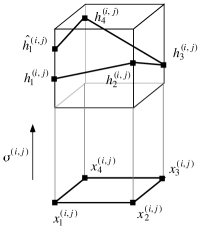
Figure 1: Path of the horizontal lift $\tilde{\gamma}$ of $\gamma$ in ${\bf E}_{\Lambda}$

Definition 2.4

Let $(\xi_{\Lambda},\omega)$ be a classical lattice model $\gamma:[0,1]\to{\bf B}$ be a path and $\langle x_{0}x_{1}\rangle$ be the corresponding path in $\Lambda$. The lattice parallel translation along the path $\gamma$ is a map

$$\tau_{\langle x_{0}x_{1}\rangle}:\pi_{\Lambda}^{-1}(x_{0})\to\pi_{\Lambda}^{-1}(x_{1}):h_{0}\mapsto h_{1}$$

where $h_{1}$ denotes the parallel transport of $h_{0}$ along the horizontal lift $\tilde{\gamma}$ of $\gamma$, i.e. $\tilde{\gamma}(0)=h_{0}$ and $h_{1}:=\tilde{\gamma}(1)$.

Let $(\xi_{\Lambda},\omega)$ be a classical lattice model, $\sigma:U\to{\bf E}_{\Lambda}$ be a local section. One obtains the lattice parallel translation $\tau_{\langle x_{0}x_{1}\rangle}$ in terms of the local connection one-form $\bar{\omega}=\sigma^{\ast}\omega$

$$\tau_{\langle x_{0}x_{1}\rangle}:h_{0}\mapsto h_{1}=h_{0}\circ{\bf P}\exp\left(-\int_{x_{0}}^{x_{1}}j^{\ast}\bar{\omega}\right),$$ (1)

where the boundary condition of the horizontal lift function

$$g(t)={\bf P}\exp\left(-\int_{x(0)}^{x(t)}j^{\ast}\bar{\omega}\right),$$

has been set to $g(0):=e$.

Definition 2.5

Let $(\xi_{\Lambda},\omega)$ be a classical lattice model. To each $1$-cell one can assign a lattice parallel translation which leads to a map

$$\langle xy\rangle\mapsto\tau_{\langle xy\rangle}$$

which is called a gauge field on $\Lambda$. The collection $\{\tau_{\langle xy\rangle}\}$ of all this lattice parallel translations is called configuration on $\Lambda$.

In general one cannot define a global gauge field on $\Lambda$ except the bundle $\xi_{\Lambda}$ is a trivial bundle. Therefore a configuration contains elements which belong to different local trivialisations.

Definition 2.6

Let $\Lambda$ be a complex such that the realization of $\Lambda$ is the 2-Torus ${\rm T}^{2}$. A directed complex $\Lambda$ with

1. $0$-cells $\{i,j\}$,

2. $1$-cells $(i,i+1)\times\{j\}$ and $\{i\}\times(j,j+1)$

3. $2$-cells $(i,i+1)\times(j,j+1)$

for all $i\in{\mathbb{Z}}_{M}$ and $j\in{\mathbb{Z}}_{N}$ is called a cubic lattice on ${\rm T}^{2}$ and is denoted by $\Lambda(N,M)$. The closure of a $2$-cell $(i,i+1)\times(j,j+1)$ is called plaquette and is denoted $\Lambda_{(i,j)}$.

Since the 2-Torus ${\rm T}^{2}$ cannot be covered by a single chart we choose an atlas

$${\cal A}({\rm T}^{2}):=\{(U_{(i,j)},\varphi_{(i,j)}){\,|\,}0\leq i\leq M-1,0\leq j\leq N-1\}$$

where the charts be all the open subsets $U_{(i,j)}\subset{\rm T}^{2}$ which cover the corresponding $2$-cells $(i,i+1)\times(j,j+1)$.

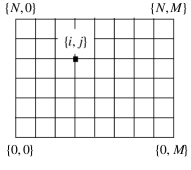
Figure 2: Cubic lattice on ${\rm T}^{2}$

Let $U_{(i,j)}$ be a chart on ${\rm T}^{2}$. We denote the corresponding local section/trivialisation by $\sigma^{(i,j)}(x)=\phi^{(i,j)}(x,g^{(i,j)})$ and $\phi^{(i,j)}$, respectively. The local connection one-form is denoted by $\bar{\omega}^{(i,j)}$. Since we denote an open interval by $(i,j)$ a site is denoted by $\{i,j\}\in{\rm T}^{2}$.

To make the lattice bundle $\xi_{\Lambda}$ unique one has to fix the collection of all transition functions $\{t_{(i,j)(k,l)}(x)\}$. Our goal is to reconstruct the transition functions, i.e. lattice bundle, from a given configuration of the lattice model.

In order to define our ${\rm U}(1)$ gauge theory over ${\rm T}^{2}$ one needs to specify a global connection one-form

$$\omega:{\bf T}{\bf E}\to{\rm i}{\mathbb{R}}.$$

Since we are interested in a connection form which has a trivial topological structure in a local trivialisation $\phi^{(i,j)}$ (no topological structure below a certain scale) we define the local connection one-forms to be

$$\bar{\omega}^{(i,j)}{\,\left|{}_{U_{(i,j)}}\right.\,}=\sigma^{(i,j)\ast}\omega:={t^{(i,j)}}^{-1}(p)\circ\mbox{\rm d}t^{(i,j)}(p),$$ (2)

for all $p\in U_{(i,j)}$, i.e. the local connection one-form restricted to the chart $U_{(i,j)}$ has to be a pure gauge in the local trivialisation $\phi^{(i,j)}$. This connection together with the lattice bundle $\xi_{\Lambda(M,N)}=({\bf E}_{\Lambda},\pi_{\Lambda},\Lambda(M,N))$ defines our model $(\xi_{\Lambda(M,N)},\omega)$.

Since the choice of all the $g^{(i,j)}$ is arbitrary this leads to $N\cdot M$ degrees of freedom. The choice of the $g^{(i,j)}$ is equivalent to the choice of the local trivialisations $\phi^{(i,j)}$, but due to left invariance of our connection one-form (Cartan Maurer form) the final result does not depend on these degrees.

3 Reconstruction of the Bundle

This property of the connection one-form $\omega$ leads to some restrictions in the choice of local trivialisations. In general, the only information one has are the ’transporters’ which are assigned to each link of the lattice, i.e. the configuration of the lattice model. Since we have an atlas ${\cal A}({\rm T}^{2})$ of the torus one has to be careful how to assign the ’transporters’ to the given charts.

Lemma 3.1

Let $(\xi_{\Lambda(M,N)},\omega)$ be our lattice model. Let $U_{(i,j)}$ be a chart on ${\rm T}^{2}$ and $\Lambda_{(i,j)}$ the corresponding plaquette. Let ${\cal A}({\rm T}^{2})$ be our atlas of ${\rm T}^{2}$ and

$$\omega^{(i,j)}{\,\left|{}_{U_{(i,j)}}\right.\,}=\sigma^{(i,j)\ast}\omega:={t^{(i,j)}}^{-1}(p)\circ\mbox{\rm d}t^{(i,j)}(p)$$

our local connection one-form. Let $\{\tau\}$ be a configuration. Only three of the four lattice parallel translations

$$\tau^{(i,j)}_{\langle x_{1}x_{2}\rangle},\,\tau^{(i,j)}_{\langle x_{2}x_{3}\rangle},\,\tau^{(i,j)}_{\langle x_{3}x_{4}\rangle}\,\mbox{and}\,\,\,\tau^{(i,j)}_{\langle x_{4}x_{1}\rangle}$$

which belong to the plaquette $\Lambda_{(i,j)}$ can be assigned to the corresponding local trivialisation $\phi^{(i,j)}$, i.e. belong to the same local representation.

Proof.

Since the local connection one-form $\omega^{(i,j)}{\,\left|{}_{U_{(i,j)}}\right.\,}$ is a pure gauge the lattice parallel translations around the plaquette must be closed. Therefore the lattice parallel translation $\tau^{(i,j)}_{\gamma}$ has to be the group identity $e$, thus three of the four lattice parallel translations have to be given in the local trivialisation and the fourth has to be the inverse of the composition of the given three. ∎

The next step is to reconstruct the transition functions $\{t_{(i,j)(k,l)}(x)\}$ from a given configuration of the lattice model.

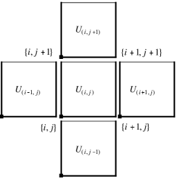
Figure 3: Choice of the charts

Take a local section $\sigma^{(i,j)}$ together with the four neighboring local sections $\sigma^{(i-1,j)}$, $\sigma^{(i+1,j)}$, $\sigma^{(i,j-1)}$ and $\sigma^{(i,j+1)}$.

Denote the transition function which maps from the fiber ${\rm U}(1)$ in the local trivialisation $\phi^{(i-1,j)}$ to the same fiber in the local trivialisation $\phi^{(i,j)}$ at $\{k,l\}$ by

$$t_{(i,j)(i-1,j)}(\{k,l\}),$$

we obtain the following relation for the elements $h^{(i-1,j)}(\{k,l\})$ and $h^{(i,j)}(\{k,l\})$ of ${\rm U}(1)$:

$$h^{(i-1,j)}(\{k,l\})=h^{(i,j)}(\{k,l\})\circ t_{(i,j)(i-1,j)}(\{k,l\}).$$ (3)

Since we want to calculate the transition function from the local sections we rewrite (3) to obtain

$$t_{(i,j)(i-1,j)}(\{k,l\})={h^{(i,j)}}^{-1}(\{k,l\})\circ h^{(i-1,j)}(\{k,l\}).$$ (4)

In each local trivialisation $\phi^{(i,j)}$ the local connection one-form $\omega^{(i,j)}{\,\left|{}_{U_{(i,j)}}\right.\,}$ has to be a pure gauge.

We choose our charts according to Fig. 3 where the three links which correspond to the three lattice parallel translation which are assigned to the corresponding local trivialisation $\phi^{(k,l)}$ are marked as bold lines.

In a trivialisation $\phi^{(i,j)}$ we can express the lattice parallel translation in terms of the local connection one-form $\bar{\omega}^{(i,j)}$ by

$$\tau^{(i,j)}_{\langle x_{1}x_{2}\rangle}:h_{1}^{(i,j)}\mapsto h_{2}^{(i,j)}=h_{1}^{(i,j)}\circ{\bf P}\exp\left(-\int_{x_{0}}^{x_{1}}j^{\ast}\bar{\omega}^{(i,j)}\right).$$ (5)

Since we have one degree of freedom per local trivialisation we choose

$$h_{1}^{(i,j)}:=g^{(i,j)}$$

where $g^{(i,j)}$ is an arbitrary ${\rm U}(1)$-element.

Denote the three lattice parallel translations along the links $\langle x_{1}x_{2}\rangle$, $\langle x_{2}x_{3}\rangle$ and $\langle x_{1}x_{4}\rangle$ by $\tau^{(i,j)}_{\langle x_{1}x_{2}\rangle},\tau^{(i,j)}_{\langle x_{2}x_{3}\rangle}$ and $\tau^{(i,j)}_{\langle x_{1}x_{4}\rangle}$, respectively. The fourth lattice parallel translation is nothing but

$$\tau^{(i,j)}_{\langle x_{3}x_{4}\rangle}:=\tau^{(i,j)}_{\langle x_{3}x_{2}\rangle}\circ\tau^{(i,j)}_{\langle x_{2}x_{1}\rangle}\circ\tau^{(i,j)}_{\langle x_{1}x_{4}\rangle},$$

since our local connection one-form has to be a pure gauge.

Table 1: Notation of local coordinates $x$ and fiber elements $h$ in different charts

point of ${\rm T}^{2}$	$U_{(i,j)}$	$U_{(i-1,j)}$	$U_{(i+1,j)}$	$U_{(i,j-1)}$	$U_{(i,j+1)}$
$\{i,j\}$	$x_{1}^{(i,j)}$	$x_{2}^{(i-1,j)}$	-	$x_{4}^{(i,j-1)}$	-
$\{i+1,j\}$	$x_{2}^{(i,j)}$	-	$x_{1}^{(i+1,j)}$	$x_{3}^{(i,j-1)}$	-
$\{i+1,j+1\}$	$x_{3}^{(i,j)}$	-	$x_{4}^{(i+1,j)}$	-	$x_{2}^{(i,j+1)}$
$\{i,j+1\}$	$x_{4}^{(i,j)}$	$x_{3}^{(i-1,j)}$	-	-	$x_{1}^{(i,j+1)}$
$\{i,j\}$	$h_{1}^{(i,j)}$	$h_{2}^{(i-1,j)}$	-	$h_{4}^{(i,j-1)}$	-
$\{i+1,j\}$	$h_{2}^{(i,j)}$	-	$h_{1}^{(i+1,j)}$	$h_{3}^{(i,j-1)}$	-
$\{i+1,j+1\}$	$h_{3}^{(i,j)}$	-	$h_{4}^{(i+1,j)}$	-	$h_{2}^{(i,j+1)}$
$\{i,j+1\}$	$h_{4}^{(i,j)}$	$h_{3}^{(i-1,j)}$	-	-	$h_{1}^{(i,j+1)}$

We ’transport’ the element $g^{(i,j)}$ at $x_{1}^{(i,j)}$ via these lattice parallel translations to obtain the fiber elements at all sites (c.f. Fig. 1) of this plaquette:

$$\begin{array}[]{l}h_{1}^{(i,j)}:=g^{(i,j)},\\ h_{2}^{(i,j)}=g^{(i,j)}\circ\tau^{(i,j)}_{\langle x_{1}x_{2}\rangle},\\ h_{3}^{(i,j)}=g^{(i,j)}\circ\tau^{(i,j)}_{\langle x_{1}x_{2}\rangle}\circ\tau^{(i,j)}_{\langle x_{2}x_{3}\rangle},\\ h_{4}^{(i,j)}=g^{(i,j)}\circ\tau^{(i,j)}_{\langle x_{1}x_{4}\rangle}.\\ \end{array}$$

Now we calculate the transition functions from the local trivialisations $\phi^{(i,j)}$.

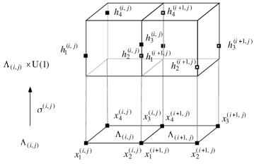
Figure 4: Notation of the local sections

Each site is covered by four charts. The first step is to recognize that only three of the four transition functions have to be calculated since the cocycle conditions give some additional relations.

We use the charts according to Fig. 3 and summarize the notation of the local coordinates in Table 1.

Our choice of charts gives the two relations

$$\tau^{(i,j)}_{\langle x_{3}x_{2}\rangle}=\tau^{(i+1,j)}_{\langle x_{4}x_{1}\rangle}\quad\mbox{and}\quad\tau^{(i,j)}_{\langle x_{4}x_{1}\rangle}=\tau^{(i-1,j)}_{\langle x_{3}x_{2}\rangle},$$ (6)

which can be used to simplify the results. Also in the non-Abelian case they are useful because if one calculates Chern classes one takes the trace over the transition functions.

For the Abelian case together with the two relations of (6) and with the use of (4) we obtain:

• Site $\{i,j\}$

  $$t_{(i,j)(i-1,j)}(\{i,j\}) = {g^{(i,j)}}^{-1}\circ g^{(i-1,j)}\circ\tau^{(i-1,j)}_{\langle x_{1}x_{2}\rangle}$$

  $$t_{(i,j)(i,j-1)}(\{i,j\}) = {g^{(i,j)}}^{-1}\circ g^{(i,j-1)}\circ\tau^{(i,j-1)}_{\langle x_{1}x_{4}\rangle}$$ (7)

• Site $\{i+1,j\}$

  $$t_{(i,j)(i,j-1)}(\{i+1,j\}) = \tau^{(i,j)}_{\langle x_{2}x_{1}\rangle}\circ{g^{(i,j)}}^{-1}\circ g^{(i,j-1)}\circ\tau^{(i,j-1)}_{\langle x_{1}x_{2}\rangle}\circ\tau^{(i,j-1)}_{\langle x_{2}x_{3}\rangle}$$

  $$t_{(i,j)(i+1,j)}(\{i+1,j\}) = \tau^{(i,j)}_{\langle x_{2}x_{1}\rangle}\circ{g^{(i,j)}}^{-1}\circ g^{(i+1,j)}$$ (8)

• Site $\{i+1,j+1\}$

  $$t_{(i,j)(i+1,j)}(\{i+1,j+1\}) = \tau^{(i,j)}_{\langle x_{2}x_{1}\rangle}\circ{g^{(i,j)}}^{-1}\circ g^{(i+1,j)}$$ (9)

  $$t_{(i,j)(i,j+1)}(\{i+1,j+1\}) = \tau^{(i,j)}_{\langle x_{3}x_{2}\rangle}\circ\tau^{(i,j)}_{\langle x_{2}x_{1}\rangle}\circ{g^{(i,j)}}^{-1}\circ g^{(i,j+1)}\circ\tau^{(i,j+1)}_{\langle x_{1}x_{2}\rangle}$$

• Site $\{i,j+1\}$

  $$t_{(i,j)(i,j+1)}(\{i,j+1\}) = \tau^{(i,j)}_{\langle x_{4}x_{1}\rangle}\circ{g^{(i,j)}}^{-1}\circ g^{(i,j+1)}$$

  $$t_{(i,j)(i-1,j)}(\{i,j+1\}) = {g^{(i,j)}}^{-1}\circ g^{(i-1,j)}\circ\tau^{(i-1,j)}_{\langle x_{1}x_{2}\rangle}$$ (10)

4 Topological Invariants

The Chern character is used to measure the twist of a bundle. Integrating the first Chern character ${\rm ch}_{1}(\mathchoice{\mbox{$\sf\displaystyle F$}}{\mbox{$\sf\textstyle F$}}{\mbox{$\sf\scriptstyle F$}}{\mbox{$\sf\scriptscriptstyle F$}})$ over the whole lattice gives an integer called Chern number

$${\rm Ch}(\xi_{\Lambda(M,N)}):=\int_{{\rm T}^{2}}{\rm ch}_{1}(\mathchoice{\mbox{$\sf\displaystyle F$}}{\mbox{$\sf\textstyle F$}}{\mbox{$\sf\scriptstyle F$}}{\mbox{$\sf\scriptscriptstyle F$}})=\frac{{\rm i}}{2\pi}\int_{{\rm T}^{2}}\mathchoice{\mbox{$\sf\displaystyle F$}}{\mbox{$\sf\textstyle F$}}{\mbox{$\sf\scriptstyle F$}}{\mbox{$\sf\scriptscriptstyle F$}},$$

which is a topological invariant and which can be used to classify the ${\rm U}(1)$-bundles over $\Lambda(M,N)$.

One has to be careful if integrating over $\Lambda(M,N)$ since our bundle is constructed by patching together local pieces via the transition functions. One also should remember that integration of a $n$-form over a manifold is done via integration over $n$-cells in the corresponding complex. Let $\bar{\omega}$ be a $2$-form and $j:\Lambda(M,N)\to{\rm T}^{2}$. Then one writes simply

$$\int_{{\rm T}^{2}}\bar{\omega}$$

for

$$\int_{{\rm T}^{2}}\bar{\omega}:=\int_{\Lambda(M,N)}j^{\ast}\bar{\omega},$$

because the integral is independent of the cellular subdivision.

Let $\{\lambda_{(i,j)}\}$ be a partition of unity subordinate to the covering $\{U_{(i,j)}\}$. Then our pullback global connection one-form can be written as

$$\bar{\omega}:=\sum_{(i,j)\in{\mathbb{Z}}_{M}\times{\mathbb{Z}}_{N}}\lambda_{(i,j)}\,\bar{\omega}=\sum_{(i,j)\in{\mathbb{Z}}_{M}\times{\mathbb{Z}}_{N}}\bar{\omega}_{(i,j)}.$$ (11)

Therefore we get

$$\mathchoice{\mbox{$\sf\displaystyle F$}}{\mbox{$\sf\textstyle F$}}{\mbox{$\sf\scriptstyle F$}}{\mbox{$\sf\scriptscriptstyle F$}}=\mbox{\rm d}\,\bar{\omega}=\sum_{(i,j)\in{\mathbb{Z}}_{M}\times{\mathbb{Z}}_{N}}\mbox{\rm d}\,\bar{\omega}_{(i,j)}.$$

Integration is now be done via partition of unity by

$$\int_{{\rm T}^{2}}\mathchoice{\mbox{$\sf\displaystyle F$}}{\mbox{$\sf\textstyle F$}}{\mbox{$\sf\scriptstyle F$}}{\mbox{$\sf\scriptscriptstyle F$}}:=\sum_{(i,j)\in{\mathbb{Z}}_{M}\times{\mathbb{Z}}_{N}}\int_{U_{(i,j)}}\mbox{\rm d}\,\bar{\omega}_{(i,j)}.$$

Since our lattice model $(\xi_{\Lambda(M,N)},\omega)$ is designed in such a way that there is no topological structure below a certain scale we have

$$\bar{\omega}^{(i,j)}:=\bar{\omega}^{(i,j)}{\,\left|{}_{U_{(i,j)}}\right.\,}=\sigma^{(i,j)\ast}\omega:={g^{(i,j)}}^{-1}(x)\circ\mbox{\rm d}g^{(i,j)}(x),$$

for all $x\in U_{(i,j)}$. We notice that the part of our pullback global connection one-form with compact support on $U_{(i,j)}$ denoted by $\bar{\omega}_{(i,j)}$ is obtained by rewriting

$$\bar{\omega}{\,\left|{}_{U_{(i,j)}}\right.\,}=\bar{\omega}_{(i,j)}+\sum_{\mbox{\scriptsize neighbors}}\bar{\omega}_{(k,l)}{\,\left|{}_{U_{(i,j)}\cap U_{(k,l)}}\right.\,}.$$

to get

$$\bar{\omega}_{(i,j)}=\bar{\omega}{\,\left|{}_{U_{(i,j)}}\right.\,}-\sum_{\mbox{\scriptsize neighbors}}\bar{\omega}_{(k,l)}{\,\left|{}_{U_{(i,j)}\cap U_{(k,l)}}\right.\,}.$$

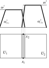
Figure 5: Partition of the connection one-form

Let $(\xi_{\Lambda(M,N)},\omega)$ be our lattice model. Take overlapping charts $U_{1}$ and $U_{2}$ on ${\rm T}^{2}$ and let $\bar{\omega}^{1}$ and $\bar{\omega}^{2}$ be the local connection one-form on $U_{1}$ and $U_{2}$, respectively. Let $\{\lambda_{(i)}\}$ be a partition of unity subordinate to the covering $\{U_{i}\}$. The corresponding pullback connection one-form is $\bar{\omega}{\,\left|{}_{U_{1}\cup U_{2}}\right.\,}=\bar{\omega}_{(1)}+\bar{\omega}_{(2)}$. With the two relations

$$\bar{\omega}_{(1)}=\bar{\omega}{\,\left|{}_{U_{1}}\right.\,}-\bar{\omega}_{(2)}{\,\left|{}_{U_{1}\cap U_{2}}\right.\,}$$

and

$$\bar{\omega}_{(2)}=\bar{\omega}{\,\left|{}_{U_{2}}\right.\,}-\bar{\omega}_{(1)}{\,\left|{}_{U_{1}\cap U_{2}}\right.\,}$$

the integral

$$\int_{U_{1}\cup U_{2}}\mbox{\rm d}\,\bar{\omega} = \int_{U_{1}}\mbox{\rm d}\,\bar{\omega}_{(1)}+\int_{U_{2}}\mbox{\rm d}\,\bar{\omega}_{(2)}$$

$$= \int_{U_{1}}\mbox{\rm d}\,\bar{\omega}{\,\left|{}_{U_{1}}\right.\,}-\int_{U_{1}}\mbox{\rm d}\,\bar{\omega}_{(2)}{\,\left|{}_{U_{1}\cap U_{2}}\right.\,}$$

$$+\int_{U_{2}}\mbox{\rm d}\,\bar{\omega}{\,\left|{}_{U_{2}}\right.\,}-\int_{U_{2}}\mbox{\rm d}\,\bar{\omega}_{(1)}{\,\left|{}_{U_{1}\cap U_{2}}\right.\,}$$

expands to

$$\int_{U_{1}\cup U_{2}}\mbox{\rm d}\,\bar{\omega}=-\int_{U_{1}}\mbox{\rm d}\,\bar{\omega}_{(2)}{\,\left|{}_{U_{1}\cap U_{2}}\right.\,}-\int_{U_{2}}\mbox{\rm d}\,\bar{\omega}_{(1)}{\,\left|{}_{U_{1}\cap U_{2}}\right.\,},$$

where we had assumed that the local connection forms have to be pure gauges, i.e. $\mbox{\rm d}\,\bar{\omega}^{1}{\,\left|{}_{U_{1}}\right.\,}\equiv 0$ and $\mbox{\rm d}\,\bar{\omega}^{2}{\,\left|{}_{U_{2}}\right.\,}\equiv 0$. Applying Stokes’ theorem gives

$$\int_{U_{1}\cup U_{2}}\mbox{\rm d}\,\bar{\omega}=-\int_{\partial U_{1}}\bar{\omega}_{(2)}{\,\left|{}_{U_{1}\cap U_{2}}\right.\,}-\int_{\partial U_{2}}\bar{\omega}_{(1)}{\,\left|{}_{U_{1}\cap U_{2}}\right.\,}.$$

Finally we realize (c.f. Fig 5) that at the boundaries of $U_{1}$ and $U_{2}$ only the local connections $\bar{\omega}^{2}$ and $\bar{\omega}^{1}$, respectively, count.

Note that due to the left invariance of our local connection one-form we have with $\tilde{t}(x)=g\circ t(x)$ and $g$ constant

$$t^{-1}(x)\circ\mbox{\rm d}\,t(x)=\tilde{t}^{-1}(x)\circ\mbox{\rm d}\,\tilde{t}(x).$$ (12)

We further notice that due to the definition of the integral over a cell-complex our map $j$ is an inclusion and can be omitted. Therefore we get

$$\int_{U_{1}\cup U_{2}}\mbox{\rm d}\,\bar{\omega}=-\int_{\langle x_{1}x_{2}\rangle}\bar{\omega}^{2}-\int_{\langle x_{2}x_{1}\rangle}\bar{\omega}^{1},$$

and together with

$$\bar{\omega}^{1}=\bar{\omega}^{2}+t_{21}^{-1}\circ\,\mbox{\rm d}\,t_{21},$$

the result

$$\int_{U_{1}\cup U_{2}}\mbox{\rm d}\,\bar{\omega} = -\int_{\langle x_{1}x_{2}\rangle}\bar{\omega}^{2}-\int_{\langle x_{2}x_{1}\rangle}\bar{\omega}^{2}-\int_{\langle x_{2}x_{1}\rangle}t_{21}(x)^{-1}\circ\,\mbox{\rm d}\,t_{21}(x)$$

$$= -\int_{\langle x_{2}x_{1}\rangle}t_{21}(x)^{-1}\circ\,\mbox{\rm d}\,t_{21}(x)$$

$$= \log t_{21}(x_{1})-\log t_{21}(x_{2}).$$

If we further assume that

$$|\int_{U_{1}\cup U_{2}}\mbox{\rm d}\,\bar{\omega}|<\pi$$ (13)

then the above equation can be written as

$$\int_{U_{1}\cup U_{2}}\mbox{\rm d}\,\bar{\omega}=\log\left(t_{21}(x_{1})\circ t_{21}^{-1}(x_{2})\right),$$ (14)

where $\log(t_{21}(x_{1})\circ t_{21}^{-1}(x_{2}))$ is defined as the principal value with range $[-\pi,\pi)$. From (13) follows that $t_{21}(x_{1})\circ t_{21}^{-1}(x_{2})\not=-1$. As we will see later there can be configurations on $\Lambda$ which violate assumption (13). Since the values of each transition function $t_{(i,j)(k,l)}(x)$ are only known on the two end points of the region of integration, a parameterization of ${\rm U}(1)$, such that at least

$$|\int_{U_{1}\cup U_{2}}\mbox{\rm d}\,\bar{\omega}|\leq\pi$$

holds, can always be assumed. Note that this assumption is an addition to (2).

Due to the fact that on $U_{(i,j)}\cap U_{(k,l)}$ the local connection one-forms are related as

$$\bar{\omega}^{(k,l)}(x)=\bar{\omega}^{(i,j)}(x)+t_{(i,j)(k,l)}^{-1}(x)\circ\mbox{\rm d}\,t_{(i,j)(k,l)}(x),$$

we obtain:

$$\int_{{\rm T}^{2}}\mathchoice{\mbox{$\sf\displaystyle F$}}{\mbox{$\sf\textstyle F$}}{\mbox{$\sf\scriptstyle F$}}{\mbox{$\sf\scriptscriptstyle F$}} = -\sum_{\langle x_{a}x_{b}\rangle}\int_{\langle x_{a}x_{b}\rangle}t_{(i,j)(k,l)}(x)^{-1}\circ\mbox{\rm d}\,t_{(i,j)(k,l)}(x)$$

$$= -\sum_{\langle x_{a}x_{b}\rangle}\left[\log t_{(i,j)(k,l)}(x_{b})-\log t_{(i,j)(k,l)}(x_{a})\right],$$

where the sum is over all directed links $\langle x_{a}x_{b}\rangle$ according to Fig. 6.

Thus the Chern number is

$${\rm Ch}(\xi_{\Lambda(M,N)})=\frac{{\rm i}}{2\pi}\sum_{\langle x_{a}x_{b}\rangle}\left[\log t_{(i,j)(k,l)}(x_{a})-\log t_{(i,j)(k,l)}(x_{b})\right].$$ (15)

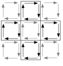
Figure 6: Orientation of the plaquettes

When integrating over all links one should remember that our lattice is a directed complex, i.e. we have an orientation (c.f. Fig. 6).

Let $M$ and $N$ be even integers, then the Chern number (c.f. (15)) gives

$${\rm Ch}(\xi_{\Lambda}) = \frac{{\rm i}}{2\pi}\sum_{\{\bar{\imath},\bar{\jmath}\}}\left[\log t_{(i,j)(i,j-1)}(\{i,j\})-\log t_{(i,j)(i,j-1)}(\{i+1,j\})\right]$$

$$+ \frac{{\rm i}}{2\pi}\sum_{\{\bar{\imath},\bar{\jmath}\}}\left[\log t_{(i,j)(i,j+1)}(\{i+1,j+1\})-\log t_{(i,j)(i,j+1)}(\{i,j+1\})\right]$$

$$+ \frac{{\rm i}}{2\pi}\sum_{\{\bar{\imath},\bar{\jmath}\}}\left[\log t_{(i,j)(i-1,j)}(\{i,j+1\})-\log t_{(i,j)(i-1,j)}(\{i,j\})\right]$$

$$+ \frac{{\rm i}}{2\pi}\sum_{\{\bar{\imath},\bar{\jmath}\}}\left[\log t_{(i,j)(i+1,j)}(\{i+1,j+1\})-\log t_{(i,j)(i+1,j)}(\{i+1,j\})\right],$$

where the sum is over all even or odd sites $\{\bar{\imath},\bar{\jmath}\}$. The last two sums give zero because we have

$$t_{(i,j)(i-1,j)}(\{i,j\})=t_{(i,j)(i-1,j)}(\{i,j+1\})$$

and

$$t_{(i,j)(i+1,j)}(\{i+1,j\})=t_{(i,j)(i+1,j)}(\{i+1,j+1\}).$$

If we straightforwardly insert the transition functions then this gives with the use of (12)

$${\rm Ch}(\xi_{\Lambda}) = \frac{{\rm i}}{2\pi}\sum_{\{\bar{\imath},\bar{\jmath}\}}\log\tau^{(i,j-1)}_{\langle x_{1}x_{4}\rangle}-\log\tau^{(i,j)}_{\langle x_{2}x_{1}\rangle}\circ\tau^{(i,j-1)}_{\langle x_{1}x_{2}\rangle}\circ\tau^{(i,j-1)}_{\langle x_{2}x_{3}\rangle}$$ (16)

$$+ \frac{{\rm i}}{2\pi}\sum_{\{\bar{\imath},\bar{\jmath}\}}\log\tau^{(i,j)}_{\langle x_{3}x_{2}\rangle}\circ\tau^{(i,j)}_{\langle x_{2}x_{1}\rangle}\circ\tau^{(i,j+1)}_{\langle x_{1}x_{2}\rangle}-\log\tau^{(i,j)}_{\langle x_{4}x_{1}\rangle}$$

Note that this definition of the Chern number is not lattice gauge invariant in the usual sense. This means that for a general configuration on $\Lambda$ different lattice gauges might lead to different results for the Chern number. We also note that reversing all transporters, which should lead to $-{\rm Ch}(\xi_{\Lambda})$, does in general not hold for the above result. To derive a unique result we must apply assumption (13) and obtain

$${\rm Ch}(\xi_{\Lambda}) = \frac{{\rm i}}{2\pi}\sum_{\{\bar{\imath},\bar{\jmath}\}}\log\Bigl{(}\tau^{(i,j-1)}_{\langle x_{1}x_{4}\rangle}\circ(\tau^{(i,j-1)}_{\langle x_{1}x_{2}\rangle}\circ\tau^{(i,j-1)}_{\langle x_{2}x_{3}\rangle}\circ\tau^{(i,j)}_{\langle x_{2}x_{1}\rangle})^{-1}\Bigr{)}$$ (17)

$$+ \frac{{\rm i}}{2\pi}\sum_{\{\bar{\imath},\bar{\jmath}\}}\log\Bigl{(}\tau^{(i,j+1)}_{\langle x_{1}x_{2}\rangle}\circ\tau^{(i,j)}_{\langle x_{3}x_{2}\rangle}\circ\tau^{(i,j)}_{\langle x_{2}x_{1}\rangle}\circ(\tau^{(i,j)}_{\langle x_{4}x_{1}\rangle})^{-1}\Bigr{)}$$

In (16) as well as in (17) the sum over all even sites can be replaced by the sum over all odd sites replacing $(i,j)$ by $(i,j-1)$ and $\log u$ by $-\log u^{-1}$. Finally, we rewrite the second sum such that we can take the sum instead of all even sites over all sites $\{i,j\}$ and obtain the following theorem.

Theorem 4.1

Let $(\xi_{\Lambda(M,N)},\omega)$ be our lattice model and choose the charts according to Fig. 3. The local connection one-form is a pure gauge and defined as in (2). Let the transition functions be as in ($\bullet$ ‣ 3) to ($\bullet$ ‣ 3). Assume that for each 1-cell (link)

$$|\int_{\langle x_{a}x_{b}\rangle}t_{(i,j)(k,l)}(x)^{-1}\circ\mbox{\rm d}\,t_{(i,j)(k,l)}(x)|<\pi$$

holds; i.e. for each 0-cell (site) $\{i,j\}$ we must have

$$\tau^{(i,j)}_{\langle x_{2}x_{1}\rangle}\circ\tau^{(i,j-1)}_{\langle x_{4}x_{1}\rangle}\circ\tau^{(i,j-1)}_{\langle x_{1}x_{2}\rangle}\circ\tau^{(i,j-1)}_{\langle x_{2}x_{3}\rangle}\neq-1$$

Choose $M$ and $N$ to be even integers. The Chern number of the lattice bundle $\xi_{\Lambda(M,N)}$ is then given by

$${\rm Ch}(\xi_{\Lambda})=-\frac{{\rm i}}{2\pi}\sum_{\{i,j\}}\log\left(\tau^{(i,j)}_{\langle x_{2}x_{1}\rangle}\circ\tau^{(i,j-1)}_{\langle x_{4}x_{1}\rangle}\circ\tau^{(i,j-1)}_{\langle x_{1}x_{2}\rangle}\circ\tau^{(i,j-1)}_{\langle x_{2}x_{3}\rangle}\right).$$ (18)

Proof.

Previous calculation. ∎

Note that such configurations for which the above Theorem holds are often called continuous configurations and the excluded ones are called exceptional configurations.

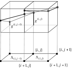
Figure 7: Two neighboring local trivialisations

If we denote the lattice parallel translations according to the standard notation in lattice field theories, i.e.

$$U_{\{i,j-1\},\hat{1}} := \tau^{(i,j-1)}_{\langle x_{1}x_{2}\rangle},$$

$$U_{\{i,j-1\},\hat{2}} := \tau^{(i,j-1)}_{\langle x_{1}x_{4}\rangle},$$

$$U_{\{i+1,j-1\},\hat{2}} := \tau^{(i,j-1)}_{\langle x_{2}x_{3}\rangle},$$

$$U_{\{i,j\},\hat{1}} := \tau^{(i,j)}_{\langle x_{1}x_{2}\rangle},$$

we obtain for (18)

$${\rm Ch}(\xi_{\Lambda})=-\frac{{\rm i}}{2\pi}\sum_{\{i,j\}}\log\left({U_{\{i,j\},\hat{1}}}^{-1}\circ{U_{\{i,j-1\},\hat{2}}}^{-1}\circ U_{\{i,j-1\},\hat{1}}\circ U_{\{i+1,j-1\},\hat{2}}\right),$$

where the logarithm

$$K_{(i,j-1)}:=\frac{{\rm i}}{2\pi}\log\left({U_{\{i,j\},\hat{1}}}^{-1}\circ{U_{\{i,j-1\},\hat{2}}}^{-1}\circ U_{\{i,j-1\},\hat{1}}\circ U_{\{i+1,j-1\},\hat{2}}\right),$$

is called the plaquette angle of the plaquette $\Lambda_{(i,j-1)}$ and corresponds to the result obtained in [22].

5 Summary

Starting with the physically reasonable assumption of a connection which is locally represented by pure gauges, we were basically able to calculate or better to assign a Chern number to each configuration on $\Lambda$. This so obtained result is unfortunately not consistent with the usual understanding of lattice gauge invariance. However even more problematic is the fact that the general result for ${\rm Ch}(\xi_{\Lambda})$ does not lead to $-{\rm Ch}(\xi_{\Lambda})$ for all configurations on $\Lambda$ when inverting all parallel translations $\tau_{\langle xy\rangle}$. These two problems can be resolved with one additional assumption on the connection which is expressed in an assumption on the parameterization of the transition functions such that the integrals over the overlap areas are less than $\pi$. This can always be assumed as far as $\tau^{(i,j)}_{\langle x_{2}x_{1}\rangle}\circ\tau^{(i,j-1)}_{\langle x_{4}x_{1}\rangle}\circ\tau^{(i,j-1)}_{\langle x_{1}x_{2}\rangle}\circ\tau^{(i,j-1)}_{\langle x_{2}x_{3}\rangle}\neq-1$ for all $\{i,j\}$. As already observed in [22] without such a condition or at least some restricting assumption there is no unique result. Depending on the parameterization of ${\rm U}(1)$ there is always one group element which, to put it crudely, allows for two results thus a tie breaker is needed.

References

[1]
M. P. Fry,
Phys. Rev. D 45 (1992) 682.
[2]
M. P. Fry,
Phys. Rev. D 47 (1993) 2629.
[3]
C. R. Gattringer and E. Seiler,
Ann. Phys. 233 (1994) 97.
[4]
H. Gausterer and C. B. Lang,
Phys. Lett. B 341 (1994) 46.
[5]
V. Azcoiti, G. D. Carlo, A. Galante, A. F. Grillo, and V. Laliena,
Phys. Rev. D 50 (1994).
[6]
M. P. Fry,
Phys. Rev. D 51 (1995) 810.
[7]
H. Gausterer and C. B. Lang,
Nucl. Phys. B 455 (1995) 785,
[8]
C. Gattringer,
and -Problem,
PhD thesis, Karl-Franzens-Universität Graz, Austria, 1995,
hep-th/9503137.
[9]
C. Gattringer,
MPI-Ph/92-52, 1995.
[10]
V. Azcoiti, G. D. Carlo, A. Galante, A. F. Grillo, and V. Laliena,
Phys. Rev. D 53 (1996) 5069,
[11]
A. C. Irving and J. C. Sexton,
Nucl. Phys. (Proc. Suppl.) 47 (1996) 679.
[12]
J. Schwinger,
Phys. Rev. 125 (1962) 397.
[13]
J. Schwinger,
Phys. Rev. 128 (1962) 2425.
[14]
S. L. Adler,
Phys. Rev. 177 (1969) 2426.
[15]
J. S. Bell and R. Jackiw,
Nuovo Cim. 60 (1969) 47.
[16]
E. Witten,
Nucl. Phys. B156 (1979) 269.
[17]
G. Veneziano,
Nucl. Phys. B 159 (1979) 213.
[18]
A. P. Balachandran et al.,
ESI 299 (1996).
[19]
H. Grosse and J. Madore,
Phys. Lett. B 283 (1992) 218.
[20]
H. Grosse, C. Klimčik, and P. Prešnajder,
Commun. Math. Phys. 178 (1996) 507.
[21]
M. Lüscher,
Commun. Math. Phys. 85 (1982) 39.
[22]
A. Phillips,
Ann. Phys. (N.Y.) 161 (1985) 399.
[23]
M. Atiyah and I. Singer,
Ann. Math. 87 (1968) 484.
[24]
E. Seiler and I. O. Stamatescu,
Phys. Rev. D25 (1982) 2177.
[25]
J. Smit and J. C. Vink,
Nucl. Phys. B 284 (1987) 234.
[26]
J. Smit and J. C. Vink,
Nucl. Phys. B 286 (1987) 485.
[27]
J. C. Vink,
Nucl. Phys. B Proc. Suppl. 4 (1988) 519.