Finite Temperature Gauge Theory on Anisotropic Lattices

1 PROBLEMS AND PROGRAM

The finite temperature transition of QCD can be seen as a change in the structure of the hadrons and as a symmetry breaking transition – a change in the structure of the vacuum (we shall take the most economical attitude that deconfining and chiral symmetry restoration are related). These phenomena are observed differently and carry complementary information. We aim at a correlated analysis involving hadronic correlators and the vacuum structure including field and density correlations, both non-trivial questions.

To understand the hadronic phenomenology at $T>0$ (see, e.g.[1]) we need to describe the dominant low energy structure in each channel. We must be prepared to cope with: wide structure replacing the well defined, $T=0$ pole; the difficulty of separating this structure from the rest of the spectrum; non-isotropic dispersion law – all intrinsic (and relevant) physical aspects. Due to breaking of the Lorentz invariance at $T>0$ we must study the general correlators. However, in lattice calculations the finite time extension $l_{\tau}=1/T$ prevents the disappearance of the higher excitations in the time propagation and more refined analyses are required. Likewise, for the description of the vacuum structure one must disentangle the physically relevant structure from UV fluctuations. We use a “gold - washing” cooling algorithm with nearly scale invariant instantons above a short range cut-off $\rho_{0}\simeq 2.3a$ [2]. Since instanton – anti-instanton (IA) pairs annihilate in any cooling their study is more sophisticated.

To allow for high $T$ with large $N_{\tau}$ but moderate $N_{\sigma}$ and $\beta$ we use anisotropic lattices:

$$a_{\sigma}/a_{\tau}=\xi>1,\ \ T=\left(\xi/N_{\sigma}\right)a_{\sigma}^{-1}$$ (1)

This ensures a fine discretization of the time axis and thus more detailed information. It also allows a fine variation of the temperature at fixed $\beta$.

We approach these questions first in quenched QCD, which shows a deconfining transition. But since chirality directly involves the quarks, in their absence the temperature effects on the hadronic correlators and on the topological structure may be delayed or modified. Therefore the final aim must be a full QCD analysis.

2 ANISOTROPIC LATTICE STUDIES

Calibration and scaling: Anisotropic lattices [3] are introduced with help of a (bare) coupling anisotropy $\gamma$, i.e. for QCD with plaquette action:

$$S_{YM}=-{{\beta}\over 3}\left[{1\over\gamma}Re\hbox{Tr}\left(P_{\sigma\sigma}\right)+\gamma Re\hbox{Tr}\left(P_{\sigma\tau}\right)\right]\$$ (2)

with $P_{\mu\nu}=W_{\mu\nu}(11)$. Euclidean symmetry should be recovered for physical quantities when expressed using the cut off anisotropy $\xi$ [3, 4]:

$$F_{n}^{\sigma}(z)=F_{n}^{\tau}(t=\xi z)$$ (3)

This fixes $\xi$ given $\gamma$ (“calibration”). If the action leads to strong artifacts, this relation cannot be fulfilled simultaneously for all observables. In a first analysis of these effects we use the tree level improved actions defined with $P$ in Eq.(2) given now by the sum of loops:

$$P_{\mu\nu}=c_{0}W_{\mu\nu}(11)+c_{1}W_{\mu\nu}(12)+c_{2}W_{\mu\nu}(22)$$ (4)

with the $W(12)$ loop averaged over directions (it is easy to see that at tree level the bare anisotropy affects all loops similarly). We compare (1): Wilson action, (2): Lüscher - Weisz Symanzik action $c_{0}=5/3,\ c_{1}=-1/12$ and (3): the “square” Symanzik action $c_{0}=16/9,\ c_{1}=-1/9,\ c_{2}=1/144$ [5]. In Table I we present $SU(2)$ results on $8^{3}\times 24$ lattices at $\gamma=3$ and $\beta=2.339,\ 1.768$ and $1.772$ (4000, 4000 and 2000 configurations respectively, separated by 10 sweeps after 10000 thermalization sweeps; $\chi^{2}$ cannot be compared between the different actions). The parameters are chosen such as to have the same cut off $a_{\sigma}$ corresponding to $\beta=2.25$ for the Wilson action at $\gamma=1$. (Notice that for the Wilson action $\Lambda(\gamma=3)\simeq 0.8\Lambda(\gamma=1)$ [3].) We fit Eq. (3) choosing for $F_{n}^{\mu}(m_{\mu})$ planar Wilson loop ratios

$$R_{n_{\sigma}}^{\mu}(m_{\mu})\equiv W_{\sigma\mu}(n_{\sigma},m_{\mu})/W_{\sigma\mu}(n_{\sigma}-1,m_{\mu}).$$ (5)

for $m_{\mu}=1,\ldots,N_{\mu}/2+1,\ \mu=\sigma,\tau$. For the Wilson action $\xi_{pert.}\simeq 3.3$, hence we have rather large non-perturbative corrections. The tree level improved actions already seem to reduce both the non-perturbative effects and the lattice artifacts. Results for $SU(3)$ and for non-planar loops and physical isotropy checks for instantons on anisotropic lattices will be reported elsewhere.

Deconfining transition: Once the calibration has been performed at $T=0$ it is assumed that $\xi$ does not depend on the lattice size, and therefore we can increase the temperature by reducing $N_{\tau}$.

$action{\vrule height=13.0pt,depth=1.4pt,width=0.0pt}$ $R_{2}{\vrule height=13.0pt,depth=1.4pt,width=0.0pt}$ $R_{3}{\vrule height=13.0pt,depth=1.4pt,width=0.0pt}$ $R_{4}{\vrule height=13.0pt,depth=1.4pt,width=0.0pt}$ $R_{5}{\vrule height=13.0pt,depth=1.4pt,width=0.0pt}$ $(1):\ \xi{\vrule height=13.0pt,depth=1.4pt,width=0.0pt}$ $4.02(6){\vrule height=13.0pt,depth=1.4pt,width=0.0pt}$ $3.90(2){\vrule height=13.0pt,depth=1.4pt,width=0.0pt}$ $3.89(2){\vrule height=13.0pt,depth=1.4pt,width=0.0pt}$ $3.93(4){\vrule height=13.0pt,depth=1.4pt,width=0.0pt}$ $\chi^{2}/d.f.{\vrule height=13.0pt,depth=1.4pt,width=0.0pt}$ $86{\vrule height=13.0pt,depth=1.4pt,width=0.0pt}$ $2{\vrule height=13.0pt,depth=1.4pt,width=0.0pt}$ $.4{\vrule height=13.0pt,depth=1.4pt,width=0.0pt}$ $.2{\vrule height=13.0pt,depth=1.4pt,width=0.0pt}$ $(2):\ \xi{\vrule height=13.0pt,depth=1.4pt,width=0.0pt}$ $3.52(3){\vrule height=13.0pt,depth=1.4pt,width=0.0pt}$ $3.44(1){\vrule height=13.0pt,depth=1.4pt,width=0.0pt}$ $3.43(2){\vrule height=13.0pt,depth=1.4pt,width=0.0pt}$ $3.42(2){\vrule height=13.0pt,depth=1.4pt,width=0.0pt}$ $\chi^{2}/d.f.{\vrule height=13.0pt,depth=1.4pt,width=0.0pt}$ $33{\vrule height=13.0pt,depth=1.4pt,width=0.0pt}$ $1{\vrule height=13.0pt,depth=1.4pt,width=0.0pt}$ $.3{\vrule height=13.0pt,depth=1.4pt,width=0.0pt}$ $.2{\vrule height=13.0pt,depth=1.4pt,width=0.0pt}$ $(3):\ \xi{\vrule height=13.0pt,depth=1.4pt,width=0.0pt}$ $3.51(1){\vrule height=13.0pt,depth=1.4pt,width=0.0pt}$ $3.46(2){\vrule height=13.0pt,depth=1.4pt,width=0.0pt}$ $3.46(3){\vrule height=13.0pt,depth=1.4pt,width=0.0pt}$ $3.45(4){\vrule height=13.0pt,depth=1.4pt,width=0.0pt}$ $\chi^{2}/d.f.{\vrule height=13.0pt,depth=1.4pt,width=0.0pt}$ $36{\vrule height=13.0pt,depth=1.4pt,width=0.0pt}$ $10{\vrule height=13.0pt,depth=1.4pt,width=0.0pt}$ $3{\vrule height=13.0pt,depth=1.4pt,width=0.0pt}$ $1.3{\vrule height=13.0pt,depth=1.4pt,width=0.0pt}$ Table I: Cut off anisotropy for $SU(2)$.

In Fig. 1 we show the Polyakov loop susceptibility as function of $\gamma$ for 3 lattice lengthes $N_{\tau}=20,18,16$ at $\beta=5.68$ (pure $SU(3)$ theory with Wilson action, $N_{\sigma}=8$).

Figure 1: Polyakov loop susceptibility $\chi$ vs $\gamma$.

Mesonic correlators near $T_{c}$: Methods for projecting onto the low energy part must be carefully defined, since a simple reweighting of the spectral function may deform a wide peak (while it would not change a pole). Using the quark propagators $S$ we measure the “wave function”

$$F^{\Gamma}({\bf P},x,t)=\sum_{\bf z}\hbox{e}^{i{\bf Pz}}\sum_{{\bf y_{1}},{\bf y_{2}}}w({\bf y_{1}},{\bf y_{2}})\times$$

$$\langle Tr\left[\Gamma S({\bf y_{1}},0;{\bf z},t)\Gamma S({\bf y_{2}},0;{\bf z}+x,t)\right]\rangle$$ (6)

Here $\Gamma$ defines the channel ($\pi,\ \rho$) and $w({\bf y_{1}},{\bf y_{2}})$ is the source, to be determined iteratively, aimed at optimizing the signal of the ground state. Pure $SU(3)$, $12^{3}\times N_{\tau}$ lattices at $\beta=5.68$ and $\gamma=4$ are used (Wilson action). At this $\gamma$ one finds $T\simeq 0.93T_{c},\ 1.03T_{c}$ and $1.15T_{c}$ with $N_{\tau}=20,\ 18$ and $16$, respectively (see Fig. 1). The calibration has been done with $N_{\tau}=72$ ($T\simeq 0$) and found $\xi\simeq 5.9$ from Wilson loops. On this $T\simeq 0$ lattice we measured also quenched pion propagators in space and time directions. They are found to show the same cut off anisotropy $\xi=5.9$ for $\gamma_{F}\equiv\kappa_{\tau}/\kappa_{\sigma}=5.4$ in the fermionic action for Wilson quarks ($\kappa$: the hopping parameter). About 20 configurations at $N_{\tau}=20$ and $18$ have been analyzed, $N_{\tau}=16$ is under way. We pursue a number of strategies:

(a) Using $F^{\Gamma}({\bf 0},x,t)$ from a simple source like point (“$pp$”: $w({\bf y_{1}},{\bf y_{2}})=\delta_{y_{1}0}\delta_{y_{2}0}$) or wall (“$ww$”: $w({\bf y_{1}},{\bf y_{2}})=1$) we fit an ansatz with three poles corresponding to the ground state exp$(-ax^{p})$ and two radial excitations [6]. We obtain in this way the wave function parameters $a,\ p$ and a first estimation of the lowest mass. These $a,\ p$ are then used to project onto the ground state at the sink.

(b) Using the same $a,\ p$ a new, shell model type source is constructed by smearing one (“$ep$”) or both (“$ee$”) quark propagators with exp$(-ax^{p})$.

(c) “Effective” masses are extracted by fitting a cosh around each t for $F^{\Gamma}({\bf 0},0,t)$ for the various sources and sinks.

(d) We make an analysis of $F^{\Gamma}({\bf 0},0,t)$ corresponding to binning of the spectral function, again using the various sources and sinks and checking the stability of the low energy structure.

(e) We analyze $F^{\Gamma}({\bf P},0,t)$ for the dispersion law.

This program is presently in work. Partial results from analyses on smaller lattices have been presented before [6]. Now we show in Fig. 2 the effective mass plots for various sources and the wave functions $F^{\Gamma}({\bf 0},x,t)$ for the “$ep$” source. There is a strong dependence of the effective mass on the sources, even in the region where it seems to saturate. This signals a low energy structure of significant width. A second observation is that there seems to be little change, both in the effective mass and in the wave function, inside few percents around $T_{c}$. Typical wave function parameters are $a=0.4,\ p=1.35$. However, before interpreting these results we want to do the full analysis, also of further quantities such as the scalar propagator and the condensate, and at a higher temperature $N_{\tau}=16$. Also a signal from free quark propagation, again a wide structure in the spectrum, may show up above $T_{c}$.

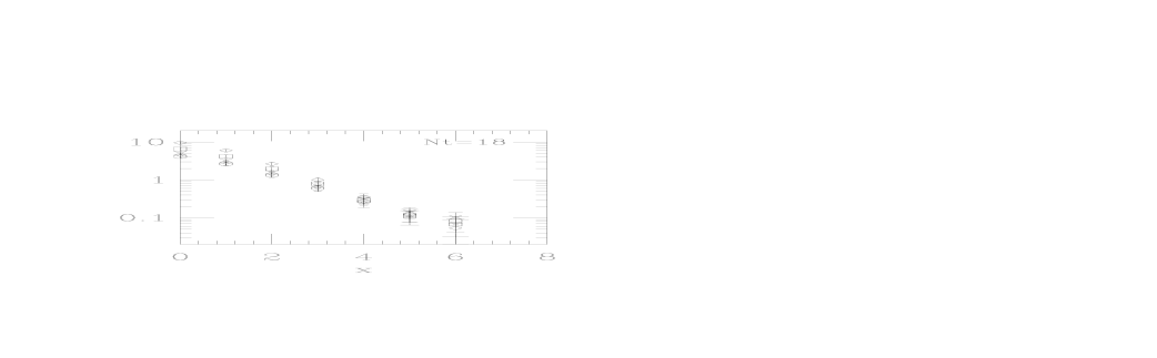
Figure 2: Pseudo-scalar effective mass vs $t$ (upper plots: “$pp$” circles, “$ep$” diamonds, “$ee$” squares, “$ww$” crosses) and “$ep$” wave function vs x, $t=1,3,5,7,10(9)$ (diamonds, bars, squares, crosses, hexagons: lower plots), at $N_{\tau}=20\ (0.93T_{c})$ and $N_{\tau}=18\ (1.03T_{c})$. No reliable estimation for the effective mass errors is available; they may be compatible with the “$ep$” - “$ee$” difference.

Acknowledgments: We are indebted to Fujitsu Ltd. for offering us computing facilities. IOS thankfully acknowledges support from DFG.

References

• [1] J. Stachel, talk at Quark Matter 96, Heidelberg, may 1996
• [2] Ph. de Forcrand, M. García Pérez and I.-O. Stamatescu, Nucl. Phys. B (Proc. Suppl.) 47 (1996) 777 and these proceedings.
• [3] F. Karsch, Nucl. Phys. B205[FS5] (1982) 239
• [4] G. Burgers, F. Karsch, A. Nakamura and I.-O. Stamatescu, Nucl.Phys. B304 (1988) 587
• [5] M. García Pérez, J. Snippe and P. van Baal, hep-lat 9608015
• [6] QCD-TARO: K. Akemi et al, Confinement 95, World Scientific, p 129