Parton Distribution Functions

Abstract

Talk at Lattice 96 Conference, St. Louis, June 1996.

Parton distribution functions give the probability to find partons (quarks and gluons) in a hadron as a function of the fraction $x$ of the proton’s momentum carried by the parton. They are conventionally defined in terms of matrix elements of certain operators. They are determined from experimental results on short distance scattering of the partons. Integrals of these functions weighted with $x^{n}$ are calculable using lattice QCD. Some simple models for their behavior have implications that could also be tested in lattice QCD.

1 Intuitive meaning of parton distribution functions

Let $d\sigma$ be a cross section involving short distances. For instance, we may consider the process hadron $A$ + hadron $B$ $\to$ jet + $X$ at the Fermilab collider. Let the jet have a high transverse momentum $P_{T}$. Intuitively, the observed jet begins as a single quark or gluon that emerges from a parton-parton scattering event with large $P_{T}$, as illustrated in Fig. 1. (Typically, this parton recoils against a single parton that carries the opposite $P_{T}$.) The large $P_{T}$ parton fragments into the observed jet of hadrons.

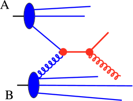
Figure 1: Hadron $A$ + hadron $B$ $\to$ 2 partons.

The physical picture illustrated in Fig. 1 suggests how we may write the cross section to produce the jet as a product of three factors. A parton of type $a$ comes from from a hadron of type $A$. It carries a fraction $x_{A}$ of the hadron’s momentum. The probability to find it is given by $f_{a/A}(x_{A})\,dx_{A}$. A second parton of type $b$ comes from a hadron of type B. It carries a fraction $x_{B}$ of the hadron’s momentum. The probability to find it is $f_{b/B}(x_{B})\,dx_{B}$. The functions $f_{a/A}(x)$ are the parton distribution functions that are the subject of this talk. The third factor is the cross section for the partons to make the observed jet, $d\hat{\sigma}$. This parton level cross section is calculated using perturbative QCD.

1.1 Factorization

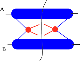
Figure 2: Factorization for hadron collisions.

We have been led by the intuitive parton picture of Fig. 1 to write the cross section for jet production in the following form

$${d\sigma\over dP_{T}}\sim$$

$${\hskip-19.91684pt}\sum_{a,b}\int\!dx_{A}\,f_{a/A}(x_{A},\mu)\ \int\!dx_{B}\,f_{b/B}(x_{B},\mu)\ {d\hat{\sigma}\over dP_{T}}.$$

Here the parton level cross section has a well behaved expansion in powers of $\alpha_{s}$,

$${d\hat{\sigma}\over dP_{T}}\sim\sum_{N}\left(\!\alpha_{s}(\mu)\over\pi\right)^{\!N}\!H_{N}(x_{A},x_{B},P_{T};a,b;\mu).$$ (2)

The coefficients $H_{N}$ are calculable in perturbative QCD.

The principle of factorization asserts that Eq. (1.1) holds up to corrections of order

$\bullet$ $(m/P_{T})^{n}$ where $m$ is a typical hadronic mass

scale and the power $n$ depends on the

process, and

$\bullet$ $\left(\alpha_{s}(\mu)\right)^{\!L}$ from truncating the expansion of

$d\hat{\sigma}/dP_{T}$.

For our purposes, we can regard factorization as an established theorem of QCD, although this subject is not without its loose ends. A review may be found in Ref. [1].

As we have seen, Eq. (1.1) has a simple intuitive meaning. However, the appearance of a parameter $\mu$ in Eq. (1.1) hints that there is more to the equation than just a model. The parameter $\mu$, which has dimensions of mass, is related to the renormalization of the strong coupling $\alpha_{s}(\mu)$ and of the operators in the definition of the parton distribution functions $f_{a/A}(x_{A},\mu)$. (Often, one uses two separate parameters in these two places.)

At the Born level, the parton level cross section $d\hat{\sigma}/dP_{T}$ is calculated in a straightforward manner. At the next-to-leading order and beyond, the calculation is not so straightforward. Various divergences appear in a naive calculation. The divergences are removed and the dependence on the scale $\mu$ appears in their place. The precise rules for calculating $d\hat{\sigma}/dP_{T}$ follow once you have set the definition of the parton distribution functions $f_{a/A}(x,\mu)$. These rules enable one to do practical calculations. For example, for jet production, the first two terms in $d\hat{\sigma}/dP_{T}$ are known in the form of computer code that puts together the pieces of Eq. (1.1) and produces a numerical cross section [2].

1.2 Reality Check

Sets of parton distribution functions, one function for each kind of parton in a proton, are produced to fit experiments. We will examine the fitting process in a later section. Fig. 3 is a graph of the gluon distribution and the up-quark distribution in a proton, according to a parton distribution set designated CTEQ3M [3]. The figure [4] shows $x^{2}f_{a/A}(x,\mu)$ for $a=g$ and $a=u$, $A=p$. Note that

$$\int_{0}^{1}dx\ x\,f_{a/A}(x,\mu)=\int d\log x\ x^{2}f_{a/A}(x,\mu),$$ (3)

so the area under the curve is the momentum fraction carried by partons of species $a$.

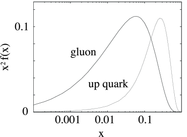
Figure 3: Gluon and up quark distributions in the proton according to the CTEQ3M parton distribution set.

1.3 Significance

Knowledge of parton distribution functions is necessary for the description of hard processes with one or two hadrons in the initial state. With two hadrons in the initial state, as at Fermilab or the future Large Hadron Collider, observed short distance cross sections take the form

$${d\sigma}\sim$$

$${\hskip-11.38092pt}\sum_{a,b}\int\!dx_{A}\,f_{a/A}(x_{A},\mu)\ \int\!dx_{B}\,f_{b/B}(x_{B},\mu)\ {d\hat{\sigma}}.$$

With one hadron in initial state, as in deeply inelastic lepton scattering at HERA (Fig. 4), the cross section has the form

$${d\sigma}\sim\sum_{a}\int dx_{A}\,f_{a/A}(x_{A},\mu)\ {d\hat{\sigma}}.$$ (5)

In either case, one has no predictions without knowledge of the parton distribution functions.

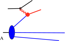
Figure 4: Deeply inelastic scattering.

The essence of Eqs. (1.3) and (5) above is that in high energy, short distance collisions a hard scattering probes the system quickly, while the strong binding forces act slowly. Thus one needs to know probabilities to find partons in a fast moving hadron as seen by an approximately instantaneous probe. This is the information encoded in the parton distribution functions. It should be evident that this information is not only useful, but also valuable in understanding hadron structure. Parton distribution functions are not everything, however. They provide a relativistic view only, a view quite different from the view that might be most economical for the description of a hadron at rest. Furthermore, they provide no information on correlations among the partons.

2 Translation to operators

We are now ready to examine the technical definition of parton distribution functions. There are, in fact, two definitions in current use. I will describe the  MS  definition, which is the most commonly used. There is also a DIS definition, in which deeply inelastic scattering plays a privileged role. The interested reader may consult the CTEQ Collaboration’s Handbook of Perturbative QCD [5] for information on the DIS definition. There are also different ways to think about the  MS  definition. In this talk, I define the parton distributions directly in terms of field operators along a light-like line, as in [6]. An equivalent construction from a different point of view may be found in [7]. As we will see, moments of the parton distribution functions are related to matrix elements of certain local operators, which appear in the operator product expansion for deeply inelastic scattering. This relation could be also used as the definition.

I distinguish between the parton distribution functions $f_{a/A}(x,\mu)$ and the structure functions $F_{1}(x,Q^{2})$, $F_{2}(x,Q^{2})$, and $F_{3}(x,Q^{2})$ that are measured in deeply inelastic lepton scattering.

2.1 Null coordinates

I will use null plane coordinates and momenta defined by

$$x^{\pm}=(x^{0}\pm x^{3})/\sqrt{2}\,,\hskip 8.5359ptP^{\pm}=(P^{0}\pm P^{3})/\sqrt{2}\,.$$ (6)

Imagine a proton with a big $P^{+}$, a small $P^{-}$, and $\vec{P}_{T}=0$. The partons in such a proton move roughly parallel to the $x^{+}$ axis, as illustrated in Fig. 5. One can treat $x^{+}$ as “time,” so that the system propagates from one plane of equal $x^{+}$ to another. For our fast moving proton, the interval in $x^{+}$ between successive interactions among the partons is typically large.

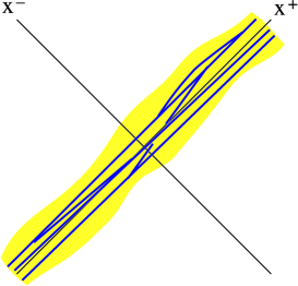
Figure 5: World lines of the partons in a fast-moving proton.

Notice that the invariant dot product between $P^{\mu}$ and $x^{\mu}$ is

$$P\cdot x=P^{+}x^{-}+P^{-}x^{+}-\vec{P}_{T}\cdot\vec{x}_{T}\,.$$ (7)

Thus the generator of “time” translations is $P^{-}$.

2.2 Null plane field theory

We will define parton distribution functions by taking a snapshot of the proton on a plane of equal $x^{+}$ in Fig. 5. To motivate the definition, we use field theory quantized on planes of equal $x^{+}$ [8]. This quantization uses the gauge $A^{+}=0$. Then the unrenormalized quark field operator $\psi_{0}$ is expanded in terms of

$\bullet$ quark destruction operators $b$ and

$\bullet$ antiquark creation operators $d^{\dagger}$

using simple spinors $w(s)$ normalized to $w^{\dagger}w=1$:

$${\scriptstyle{1\over 2}}\gamma^{-}\gamma^{+}\psi_{0}(x^{+},x^{-},\vec{x}_{T})=$$

$$\hskip-8.5359pt{1\over(2\pi)^{3}}\int_{0}^{\infty}{dk^{+}\over 2k^{+}}\,\int d\vec{k}_{T}\sum_{s}(\sqrt{2}k^{+})^{1/2}$$

$$\hskip-8.5359pt\times\biggl{\{}e^{-i\,(k^{+}x^{-}-\vec{k}_{T}\cdot\vec{x}_{T})}\,w(s)\,b(k^{+},\vec{k}_{T};s;x^{+})$$

$${}+e^{+i\,(k^{+}x^{-}-\vec{k}_{T}\cdot\vec{x}_{T})}\,w(-s)\,d^{\dagger}(k^{+},\vec{k}_{T};s;x^{+})\biggr{\}}.$$

The factor ${\scriptstyle{1\over 2}}\gamma^{-}\gamma^{+}$ here serves to project out the components of the quark field $\psi_{0}$ that are the independent dynamical operators in null plane field theory.

2.3 The quark distribution function

We are now ready to define the (unrenormalized) quark distribution function. Let $|P\rangle$ be the state vector for a hadron of type $A$ carrying momentum $P^{\mu}$. Take the hadron to be spinless in order to simplify the notation. Construct the unrenormalized distribution function for finding quarks of flavor $j$ in hadron $A$ as

$$f^{(0)}_{j/A}(x)\times\langle P^{+\prime},\vec{P}_{T}^{\prime}|P^{+},\vec{P}_{T}\rangle=$$ (9)

$$\hskip 14.22636pt{1\over 2x(2\pi)^{3}}\int d\vec{k}_{T}\sum_{s}\,\langle P^{+\prime},\vec{P}_{T}^{\prime}|$$

$$\hskip 14.22636pt\times b^{\dagger}_{j}(xP^{+},\vec{k}_{T};s;x^{+})\,b_{j}(xP^{+},\vec{k}_{T};s;x^{+})$$

$$\hskip 14.22636pt\times|P^{+},\vec{P}_{T}\rangle\ .$$

In Eq. (9) there are factors relating to the normalization of the states and the creation/destruction operators. There is a quark number operator $b^{\dagger}b$ for flavor $j$. We integrate over the quark transverse momentum $\vec{k}_{T}$ and sum over the quark spin $s$.

2.4 Translation to coordinate space

With a little algebra, we find

$$f^{(0)}_{j/A}(x)={1\over 4\pi}\int dy^{-}e^{-ixP^{+}y^{-}}$$

$$\hskip-17.07182pt\times\langle P^{+}\!,\vec{0}_{T}|\overline{\psi}_{0,j}(0,y^{-},\vec{0}_{T})\gamma^{+}{\psi}_{0,j}(0,0,\vec{0}_{T})|P^{+}\!,\vec{0}_{T}\rangle.$$

Notice that the (still unrenormalized) quark distribution function is an expectation value in the hadron state of a certain operator. The operator is not local but “bilocal.” The two points, $(0,y^{-},\vec{0}_{T})$ and $(0,0,\vec{0}_{T})$, at which the field operators are evaluated are light-like separated. The formula directs us to integrate over $y^{-}$ with the right factor so that we annihilate a quark with plus momentum $xP^{+}$.

2.5 Gauge invariance

Before turning to the renormalization of the operator that occurs in the quark distribution function, we note that the definition as it stands relies on the gluon potential $A^{\mu}(x)$ being in the gauge $A^{+}=0$. Let us modify the formula so that

$\bullet$ the operator is gauge invariant and

$\bullet$ we match the previous definition in

$A^{+}=0$ gauge.

The gauge invariant definition is

$$f^{(0)}_{j/A}(x)={1\over 4\pi}\int\!dy^{-}e^{-ixP^{+}y^{-}}\ \langle P^{+}\!,\vec{0}_{T}|$$ (11)

$$\hskip 28.45274pt\times\overline{\psi}_{0,j}(0,y^{-},\vec{0}_{T})\gamma^{+}{\cal O}_{0}\ {\psi}_{0,j}(0,0,\vec{0}_{T})$$

$$\hskip 28.45274pt\times|P^{+}\!,\vec{0}_{T}\rangle\ ,$$

where

$${\cal O}_{0}={\cal P}\exp\left(ig_{0}\int_{0}^{y^{-}}\!\!\!dz^{-}\,{A}_{0,a}^{+}(0,z^{-},\vec{0}_{T})\,t_{a}\right).$$ (12)

Here ${\cal P}$ denotes a path-ordered product, while the $t_{a}$ are the generators for the 3 representation of SU(3). There is an implied sum over the color index $a$.

2.6 Interpretation of the eikonal gauge operator

The appearance of the operator $\cal O$, Eq. (12), in the definition (11) seems to be just a technicality. However, this operator has a physical interpretation that is of some importance. Let us write this operator in the form

$${\cal O}_{0}=\overline{\cal P}\exp\left(-ig_{0}\int_{y^{-}}^{\infty}\!\!\!dz^{-}\,{A}_{0,a}^{+}(0,z^{-},\vec{0}_{T})\,t_{a}\right)$$ (13)

$$\times{\cal P}\exp\left(ig_{0}\int_{0}^{\infty}\!\!\!dz^{-}\,{A}_{0,a}^{+}(0,z^{-},\vec{0}_{T})\,t_{a}\right).$$

Inserting this form in the definition (11), we can introduce a sum over states $|N\rangle\langle N|$ between the two exponentials in Eq. (13). We take these states to represent the final states after the quark has been “measured.”

Consider now a deeply inelastic scattering experiment that is used to determine the quark distribution. The experiment doesn’t just annihilate the quark’s color. In a suitable coordinate system, a quark moving in the plus direction is struck and exits to infinity with almost the speed of light in the minus direction, as illustrated in Fig. 6. As it goes, the struck quark interacts with the gluon field of the hadron.

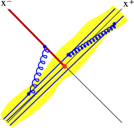
Figure 6: Effect of the eikonal gauge operator.

We can now see that the role of the operator $\cal O$ is to replace the struck quark with a fixed color charge that moves along a light-like line in the minus-direction, mimicking the motion of the actual struck quark in a real experiment.

2.7 Renormalization

We now discuss the renormalization of the operator products in the definition (11). We use  MS  renormalized fields ${\psi}(x)$ and ${A}^{\mu}(x)$ and we use the  MS  renormalized coupling $g$. The field operators are evaluated at points separated by $\Delta x$ with $\Delta x^{\mu}\Delta x_{\mu}=0$. For this reason, there will be ultraviolet divergences from the operator products. We elect to renormalize the operator products with the  MS  scheme.

For instance, Fig. 7 illustrates one of the diagrams for the distribution of quarks in a proton. Before it is measured, the quark emits a gluon into the final state. There is a loop integration over the minus and transverse components of the measured quark’s momentum. This loop integration is ultraviolet divergent. To apply  MS  renormalization, we perform the integration in $4-2\epsilon$ dimensions, including a factor $(\mu^{2}e^{\gamma}/4\pi)^{\epsilon}$ that keeps the dimension constant while supplying some conventional factors. The integral will consist of a pole term proportional to $1/\epsilon$ plus terms that are finite as $\epsilon\to 0$. We simply subtract the pole term. Notice that  MS  renormalization introduces a scale $\mu$.

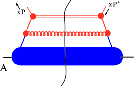
Figure 7: Renormalization of an ultraviolet divergent loop integration.

The definition of the renormalized quark distribution function is thus

$$f_{j/A}(x,\mu)={1\over 4\pi}\int dy^{-}e^{-ixP^{+}y^{-}}\ \langle P^{+},\vec{0}_{T}|$$ (14)

$$\hskip 28.45274pt\times\overline{\psi}_{j}(0,y^{-},\vec{0}_{T})\gamma^{+}{\cal O}\ {\psi}_{j}(0,0,\vec{0}_{T})$$

$$\hskip 28.45274pt\times|P^{+},\vec{0}_{T}\rangle_{{\vbox{\hrule\kern 1.0pt\hbox{\smallrm MS}}}}\,,$$

where the  MS  denotes the renormalization prescription and where

$${\cal O}={\cal P}\exp\left(ig\int_{0}^{y^{-}}\!\!\!dz^{-}\,{A}_{a}^{+}(0,z^{-},\vec{0}_{T})\,t_{a}\right).$$ (15)

2.8 Antiquarks and gluons

We now have a definition of parton distribution functions for quarks. For antiquarks, we use charge conjugation to define

$${f_{\bar{j}/A}(x,\mu)}={1\over 4\pi}\int dy^{-}e^{-ixP^{+}y^{-}}\ \langle P^{+}\!\!,\vec{0}_{T}|$$ (16)

$$\hskip 17.07182pt\times{\rm Tr}\!\left\{\!\gamma^{+}{\psi}_{j}(0,y^{-},\vec{0}_{T}){{\cal O}}\ \overline{\psi}_{j}(0,0,\vec{0}_{T})\right\}\!$$

$$\hskip 17.07182pt\times|P^{+}\!\!,\vec{0}_{T}\rangle_{\vbox{\hrule\kern 1.0pt\hbox{\smallrm MS}}}\ ,$$

where

$${{\cal O}}={\cal P}\exp\left(-ig\int_{0}^{y^{-}}\!\!\!dz^{-}\,{A}_{a}^{+}(0,z^{-},\vec{0}_{T})\,t^{T}_{a}\right).$$ (17)

For gluons we begin with the number operator in $A^{+}=0$ gauge. Proceeding analogously to the quark case, we obtain an expression involving the field strength tensor $F_{a}^{\mu\nu}$ with color index $a$:

$${f_{g/A}(x,\mu)}={1\over 2\pi\,xP^{+}}\int dy^{-}e^{-ixP^{+}y^{-}}\ \langle P^{+}\!\!,\vec{0}_{T}|$$ (18)

$$\hskip 34.14322pt\times{F}_{\!a}(0,y^{-},\vec{0}_{T})^{+\nu}{{\cal O}}_{ab}\ {F}_{\!b}(0,0,\vec{0}_{T})_{\nu}^{\ +}$$

$$\hskip 34.14322pt\times|P^{+}\!\!,\vec{0}_{T}\rangle_{\vbox{\hrule\kern 1.0pt\hbox{\smallrm MS}}}\ ,$$

where

$${{\cal O}}={\cal P}\exp\left(ig\int_{0}^{y^{-}}\!\!\!dz^{-}\,{A}_{c}^{+}(0,z^{-},\vec{0}_{T})\,t_{c}\right).$$ (19)

Here the $t_{c}$ generate the 8 representation of SU(3).

3 Renormalization group

A change in the scale $\mu$ induces a change in the parton distribution functions $f_{a/A}(x,\mu)$. The change comes from the change in the amount of ultraviolet divergence that renormalization is removing. Since the operators are non-local in $y^{-}$, the ultraviolet counterterms are integral operators in $k^{+}$ or equivalently in momentum fraction $x$. Since the ultraviolet divergences mix quarks and gluons, so do the counterterms.

One finds

$$\mu^{2}{d\over d\mu^{2}}{f_{a/A}(x,\mu)}=$$ (20)

$$\int_{x}^{1}{d\xi\over\xi}\sum_{b}\ {P_{a/b}(x/\xi,\alpha_{s}(\mu))}\ {f_{b/A}(\xi,\mu)}.$$

The Altarelli-Parisi (= GLAP = DGLAP) kernel $P_{a/b}$ is expanded in powers of $\alpha_{s}$. The $\alpha_{s}^{1}$ and $\alpha_{s}^{2}$ terms are known and used.

3.1 Renormalization group interpretation

The derivation of the renormalization group equation (20) is rather technical. One should not lose sight of its intuitive meaning. Parton splitting is always going on as illustrated in Fig. 8. A probe with low resolving power doesn’t see this splitting. The renormalization parameter $\mu$ corresponds to the physical resolving power of the probe. At higher $\mu$, field operators representing an idealized experiment can resolve the mother parton into its daughters.

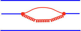
Figure 8: A quark can fluctuate into a quark plus a gluon in a small space-time volume.

3.2 Renormalization group result

One can use the renormalization group equation (20) to find the parton distributions at a scale $\mu$ if they are known at a lower scale $\mu_{0}$. Fig. 9 shows an example, the gluon distribution at $\mu=10{\ \rm GeV}$ and at $\mu=100{\ \rm GeV}$ (using the CTEQ3M parton distribution set). Notice that with greater resolution, a gluon typically carries a smaller momentum fraction $x$ because of splitting.

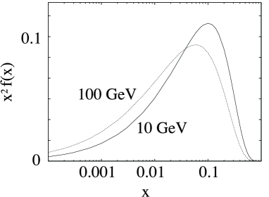
Figure 9: Evolution of the gluon distribution between $\mu=10{\ \rm GeV}$ and $\mu=100{\ \rm GeV}$.

4 Translation to local operators

We have defined the parton distributions as hadron matrix elements of certain operator products, where the operators are evaluated along a light-like line. Now we relate the parton distributions to products of operators all at the same point. It is these local operator products that were originally used in the interpretation of deeply inelastic scattering experiments. For lattice QCD, evaluation of operator products at light-like separations would be, at best, very difficult, so the translation to local operator products seems essential.

4.1 Quarks

Note that, according to the definitions (14) and (16),

$$f_{j/A}(x,\mu) = 0\,,\hskip 56.9055pt{x>1}\,,$$

$$f_{\bar{j}/A}(x,\mu) = 0\,,\hskip 56.9055pt{x>1}\,,$$

$$f_{j/A}({-x},\mu) = {-}f_{{\bar{j}}/A}(x,\mu).$$ (21)

Consider the moments of the quark/antiquark distributions defined by

$$M_{j}^{(J)}(\mu)=$$

$$\int_{0}^{1}{dx\over x}\,{x^{J}}\left\{f_{j/A}(x;\mu)+{(-1)^{J}}f_{{\bar{j}}/A}(x;\mu)\right\}$$

for $J=1,2,\dots$. Given the properties above, this is

$$M_{j}^{(J)}(\mu)=\int_{{-\infty}}^{{\infty}}{dx\over x}\,{x^{J}}f_{j/A}(x;\mu)\,.$$ (23)

Obtaining $\int_{-\infty}^{\infty}dx$ is the essential step.

From the operator definitions of the $f$s, this is

$$M_{j}^{(J)}(\mu)=$$ (24)

$${1\over 4\pi}\int dy^{-}\int_{-\infty}^{\infty}dx\ e^{-ixP^{+}{y^{-}}}\ \left({-i\over P^{+}}{{\partial\over\partial y^{-}}}\right)^{J-1}$$

$$\ \ \times\langle P|\overline{\psi}_{j}({y^{-}})\gamma^{+}{\cal O}({y^{-}},0)\ \psi_{j}(0)|P\rangle_{\vbox{\hrule\kern 1.0pt\hbox{\smallrm MS}}}\ .$$

Performing the $x$-integration gives a $\delta(y^{-})$. Thus we get a local operator. The ${\partial/\partial y^{-}}$ differentiates either the quark field or the exponential of gluon fields in $\cal O$, Eq. (15). We find

$$M_{j}^{(J)}(\mu)=$$

$$\hskip-8.5359pt{1\over 2}(P^{+})^{-J}\,\langle P|\overline{\psi}_{j}(0)\gamma^{+}\left(i{D^{+}}\right)^{J-1}\psi_{j}(0)|P\rangle_{\vbox{\hrule\kern 1.0pt\hbox{\smallrm MS}}}\,,$$

where

$${D^{\mu}}={\partial\over\partial y_{\mu}}-ig\,A^{\mu}_{a}(y)\,t_{a}\,.$$ (26)

We have now related the moments of the quark distribution to products of operators evaluated at the same point. However, this is not yet ready for the lattice because it would not be easy to differentiate the operators with respect to $y^{-}$. To obtain a more useful expression, consider ${\langle{\cal O}_{j}^{(J)}\rangle}$ defined by

$$\{P^{\mu_{1}}P^{\mu_{1}}\cdots P^{\mu_{J}}\}_{\rm TS}\ {\langle{\cal O}_{j}^{(J)}\rangle}=$$

$$\hskip-14.22636pt{1\over 2}\langle P|\overline{\psi}_{j}(0)\,\{\gamma^{\mu_{1}}iD^{\mu_{2}}\cdots iD^{\mu_{J}}\}_{\rm TS}\,\psi_{j}(0)|P\rangle_{\vbox{\hrule\kern 1.0pt\hbox{\smallrm MS}}}\ .$$

where TS denotes taking the traceless symmetric part of the tensor enclosed.

Then

$${\langle{\cal O}_{j}^{(J)}\rangle}=M_{j}^{(J)}(\mu)=$$

$$\int_{0}^{1}{dx\over x}\,{x^{J}}\left\{{f_{j/A}(x;\mu)}+(-1)^{J}{f_{\bar{j}/A}(x;\mu)}\right\}.$$

This is our final result.

We can now imagine the following program for a lattice calculation. One could measure ${\langle{\cal O}_{j}^{(J)}\rangle}$ on the lattice for $J=1,2,\dots$. Of course, this would not be so easy, but it would gives moments of the quark/antiquark distributions that could be compared to the corresponding moments of the distributions determined from experiments.

4.2 Gluons

We follow a similar analysis to relate the gluon distribution function to local operator products. From the definition (18), it follows that

$$f_{g/A}(x,\mu) = 0\,,\hskip 56.9055pt{x>1}\,,$$

$$f_{g/A}({-x},\mu) = {-}f_{g/A}(x,\mu)\,.$$ (29)

For $J=2,4,6,\dots$, we relate moment integrals over the interval $0<x<1$ to moment integrals over all $x$

$$\int_{0}^{1}\!{dx\over x}\,{x^{J}}f_{g/A}(x;\mu)={1\over 2}\int_{{-\infty}}^{{\infty}}\!{dx\over x}\,{x^{J}}f_{g/A}(x;\mu).$$ (30)

Define operator matrix elements ${\langle{\cal O}_{g}^{(J)}\rangle}$ for $J=2,4,6,\dots$ by

$$\{P^{\mu_{1}}P^{\mu_{1}}\cdots P^{\mu_{J}}\}_{\rm TS}\ \langle{\cal O}_{g}^{(J)}\rangle=$$

$$\hskip-17.07182pt{1\over 2}\langle P|\{F^{\mu_{1}\!\nu}\!(0)\,iD^{\mu_{2}}\cdots iD^{\mu_{\!J-1}}\,F_{\nu}^{\ \mu_{\!J}}\!(0)\,\}_{\rm TS}\,|P\rangle_{\vbox{\hrule\kern 1.0pt\hbox{\smallrm MS}}}\,.$$

Then these operator matrix elements are the moments of the gluon distribution:

$${\langle{\cal O}_{g}^{(J)}\rangle}=M_{g}^{(J)}(\mu)=\int_{0}^{1}{dx\over x}\,{x^{J}}{f_{g/A}(x;\mu)}\,.$$ (32)

Again, one can contemplate measuring ${\langle{\cal O}_{g}^{(J)}\rangle}$ on the lattice for $J=2,4,\dots$. The result could be compared to the corresponding moments of the phenomenological gluon distribution.

5 Determination from experiments

I have alluded several times to the fact that parton distribution functions are related to experimental results. Let us look at this in some more detail.

5.1 Example

Fig. 10 shows data for the cross section to observe one jet plus anything in high energy $p\bar{p}$ collisions. The data from the CDF Collaboration [9] are compared to theory using CTEQ3M parton distributions that did not have this data as input. (In the figure, $E_{T}$ denotes essentially the transverse momentum of the jet.)

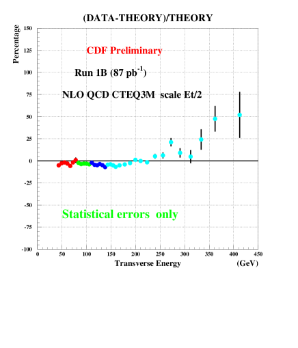
Figure 10: One jet inclusive jet cross section $d\sigma/dE_{T}$, (Data $-$ Theory)/Theory versus $E_{T}$. Source: CDF.

One notes that the data do not agree with the theory at the highest values of $E_{T}$. Does this indicate a breakdown of QCD at the smallest distances? An alternative explanation [10] is that the gluon distribution used in the theory was actually poorly constrained at large $x$ ($x\sim 0.5$) by other experiments. In support of this explanation, the CTEQ collaboration offered the theory curve shown in Fig. 11. This theory curve was obtained using modified parton distributions that still fit other data well. (Note: the data in this figure predates that in Fig. 10 and has lower statistics.)

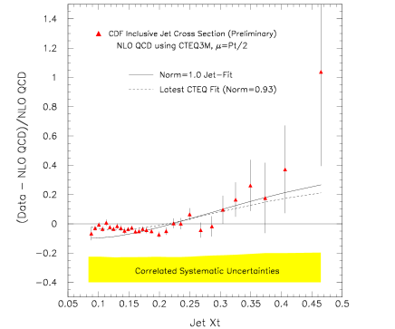
Figure 11: (Data $-$ Theory)/Theory versus $x_{T}=2E_{T}/\sqrt{s}$ for CTEQ4HJ partons, “Norm = 1.0 Jet-Fit.” Source: CTEQ.

Could a lattice measurement of moments of the gluon distribution distinguish between these possibilities? In Table 1, I show the lowest moments of the gluon distributions from the two parton distribution sets in question. The two gluon distributions are very different at large $x$, but almost the same at small $x$. Thus one has to go to the $J=6$ moment to see a substantial difference. Measurement of $M^{(6)}_{g}(2{\ \rm GeV})$ in a lattice calculation would, I think, be quite difficult.

Table 1: Moments of gluon distribution for two sample parton distributions sets

	CTEQ3M	CTEQ4HJ
$M^{(2)}_{g}(2{\ \rm GeV})$	$4.5\times 10^{-1}$	$4.3\times 10^{-1}$
$M^{(4)}_{g}(2{\ \rm GeV})$	$1.6\times 10^{-2}$	$1.9\times 10^{-2}$
$M^{(6)}_{g}(2{\ \rm GeV})$	$2.1\times 10^{-3}$	$4.4\times 10^{-3}$

5.2 What parton people do

There are three main groups currently doing “global fitting” of parton distributions:

$\bullet$ Martin, Roberts and Stirling (MRS) [11],

$\bullet$ Gluck, Reya, and Vogt (GRV) [12],

$\bullet$ Botts, Huston, Lai, Morfin, Owens, Qiu,

Tung, Weerts,…(CTEQ) [3].

Other groups have done this in the past, e.g. Duke and Owens and Eichten, Hinchliffe, Lane and Quigg.

The idea of the global fitting is to adjust the parton distribution functions to make theory and experiment agree for a wide range of processes. For example, recent CTEQ fits have used the following processes:

$e+p\to X$

$\mu+p\to X$                  $\mu+{}^{2}\!H\to X$

$\nu+Fe\to X$                $\bar{\nu}+Fe\to X$

$p+p\to\mu+\bar{\mu}+X$       $p+{}^{2}\!H\to\mu+\bar{\mu}+X$

$p+Cu\to\mu+\bar{\mu}+X$

$p+\bar{p}\to W\to\ell+\bar{\ell}+X$

$p+\bar{p}\to\gamma+X$  .

The main features of a program of global fitting are as follows. One chooses a starting scale $\mu_{0}$ (say 2  GeV ). Then one writes the $f_{a/p}(x;\mu_{0})$ in terms of several parameters for $a=g,u,\bar{u},d,\bar{d},s,\bar{s}$. (Typically the heavy quark distributions, for $a=c,\bar{c},b,\bar{b},t,\bar{t}$, are generated from evolution, not fit to data.) For example, one may choose

$$f(x;\mu_{0})=Ax^{B}(1-x)^{C}(1+Ex^{D})\,.$$ (33)

The parton distribution functions obey certain flavor and momentum sum rules, such as

$$\int_{0}^{1}dx\ \left[f_{u/p}(x,\mu)-f_{\bar{u}/p}(x,\mu)\right] = 2,$$

$$\sum_{a}\int_{0}^{1}dx\ xf_{a/p}(x,\mu) = 1.$$ (34)

These sum rules follow from the operator definitions (14), (16), (18). The parametrizations are chosen so that the flavor and momentum sum rules are obeyed exactly.

Now one picks a trial set of parameters. This determines $f(x;\mu_{0})$, from which one calculates $f(x;\mu)$ for all $\mu$ by evolution. Next, given the $f(x;\mu)$, one generates theory curves for each type of experiment used. Finally, one compares the results to the data.

This sequence is iterated, adjusting the parameters to get a good fit. There are more than 1000 data and only about 25 parameters to be fit, so the fact that this procedure works at all is an indication that QCD is the correct theory of the strong interactions.

6 Relation to lattice QCD

Let me give here a personal view about how lattice calculations of the lowest moments of parton distributions, continuing the work reported at this conference [13], might enhance our understanding of particle physics.

First, what do we know now? To a reasonable approximation, the parton distribution functions have already been determined from experiment. Furthermore, there is partial understanding of parton distributions in two limits: one has some idea about $x\to 0$ behavior from Regge physics and from the evolution equation; one has some idea about $x\to 1$ behavior from Feynman graphs. However, this understanding is of a rather limited nature. In general there is little theoretical understanding of why parton distributions are what they are.

A lattice calculation of moments of parton distributions could, first of all, test QCD. One could calculate something about hadron structure instead of simply measuring that structure. It is possible, in principle, that lattice calculations could add to the precision of parton determinations, particularly for the gluon distribution. However it seems to me that the goal of doing better by calculation than by experiment is rather distant at this point. Finally, and perhaps most importantly, it seems to me that lattice calculations might lead to an improved understanding of hadron structure by either validating or falsifying simple pictures about how the partons are arranged in a hadron. I turn to this question in the sections that follow.

7 Are partons inside “valence quarks”?

Figure 12 illustrates a simple picture of how partons might be arranged in a proton. A proton consists of three valence quarks, U U D. A valence quark in this sense is a big object. Each valence quark consists of short distance quarks and gluons. I do not know the history of this simple idea, but one illustrative paper on the subject is Ref. [14].

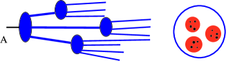
Figure 12: A hadron may contain valence quarks that in turn are made of short distance quarks and gluons.

This idea may be expressed in the formula

$${f_{a/A}(x;\mu)}=\int_{x}^{1}\!{d\xi\over\xi}\!\sum_{J=U,D}\!{F_{J/A}(\xi)}\,{f_{a/J}(x/\xi;\mu)}.$$ (35)

Here $F_{J/A}(\xi)$ represents the distribution of valence quarks of flavor $J$ in a hadron of type $A$. Then $f_{a/J}(x/\xi;\mu)\,d(x/\xi)$ is the probability to find a parton of type $a$ carrying a fraction $x/\xi$ of the valence quark’s momentum.

Note that, without an additional hypothesis for ${F_{J/A}(\xi)}$, this formula has negative predictive value: in order to predict the values of the functions $f_{a/p}(x;\mu)$ we introduce unknown functions $f_{a/J}(x/\xi;\mu)$ and $F_{J/A}(\xi)$. However, if you look not just at hadrons $p$ and $n$ but at hadrons $p,n,\pi,\rho,\omega,\dots$ then there is predictive power. There is experimental information on the distribution of hadrons in the pion from $\pi+p\to\mu^{+}+\mu^{-}+X$. In addition, there is some experimental information on the distribution of hadrons in the $\rho^{0}$ from deeply inelastic scattering from photons. However, experimental information on the distribution of partons in other hadrons is lacking. Here one sees an advantage of calculation: it is much easier to create all kinds of hadrons on a lattice than in an accelerator.

7.1 Possibilities for $F_{J/A}(x)$

One simple hypothesis for $F_{J/A}(x)$ would be that a constituent quark is simply an elementary quark as seen at a very low resolution scale $\mu$. Thus one might identify ${F_{J/A}(x)}={f_{J/A}(x,0.3{\ \rm GeV})}$. However, this hypothesis does not seem to work [12].

Another possibility is that the constituent quarks are very weakly bound in a hadron. Then

$${F_{U/p}(x)} \approx 2\,\delta(x-1/3),$$

$${F_{D/p}(x)} \approx 1\,\delta(x-1/3).$$ (36)

If one investigates only protons and neutrons, then this hypothesis has zero predictive power. (That is better, of course, than negative predictive power.) However, of one looks at $p,n,\rho,\omega...$ then there is some predictive power.

7.2 Parton correlations

The valence quark picture appears to say something about multiparton correlations. Examining Fig. (13), we see that the partons in a proton are clumped together more than they would be if they were spread throughout the proton. Thus a suitably defined two parton correlation function would be larger at short distances than it would be in an uncorrelated model.

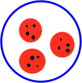
Figure 13: If the short distance partons are contained inside valence quarks, then the probability that two partons are close together is larger.

There is some experimental information about two parton correlations from double parton scattering. Such an experiment is illustrated in Fig. 14.

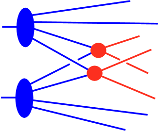
Figure 14: Parton correlations can be examined experimentally by looking for double parton scattering.

One could investigate this issue in a lattice calculation. One would define a two parton distribution function $f_{(a,b)/A}(x_{a},x_{b},r)$ where $x_{a}$ and $x_{b}$ are the momentum fractions of two partons and $r$ is the transverse separation between them. The simplest uncorrelated model (ignoring even correlations due to momentum conservation) would be that this function is the product of $f_{a/A}(x_{a})$, $f_{b/A}(x_{b})$, and a theta function that requires that both partons are not more than a distance $R$ from each other, $\theta(r<R)$. There must be more correlation than this. The question is, how much?

8 Partons in the pion cloud

Figure 15 illustrates another simple picture, usually known as the Sullivan model [15]. Sometimes a proton is a proton. Sometimes a proton is a proton plus a pion. More generally, a proton can exist virtually as a baryon plus a meson. Each baryon or meson consists of short distance quarks and gluons.

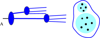
Figure 15: A physical hadron may consist of bare hadrons that in turn are made of quarks and gluons.

A formula for the parton distributions in this model is

$${f_{a/A}(x;\mu)}=\int_{x}^{1}{d\xi\over\xi}\sum_{H}{F_{H/A}(\xi)}\ {f_{a/H}(x/\xi;\mu)}.$$ (37)

Here $H$ represents hadrons that might be virtual constituents of the proton and $F_{H/A}(\xi)$ represents the distribution of these virtual hadrons in the proton. One makes a model for ${F_{H/A}(\xi)}$ based on measured meson-baryon couplings.

Note that $A$ could be a proton, a “physical proton,” while $H$ could be a proton, a “bare proton.” The relation between these is, in my opinion at least, rather murky. Nevertheless, there must be some truth to the model. If there is some truth to it, the model suggests that sometimes a hadron fluctuates to a much bigger size. Again, an investigation of multiparton correlations could help to pin the question down.

9 Conclusion

I conclude that lattice calculations continuing the work [13] presented at this conference could test QCD by predicting parton distributions directly from the QCD lagrangian. One also has the possibility of asking and answering questions about hadron structure that go beyond what can be easily measured experimentally.

References

- [1] J. C. Collins and D. E. Soper, Ann. Rev. Nucl. Part. Sci. 37 (1987) 383; J. C. Collins, D. E. Soper and G. Sterman, in A. H. Mueller, ed., Perturbative Quantum Chromodynamics (World Scientific, 1989).
- [2] S. D. Ellis, Z. Kunszt and D. E. Soper, Phys. Rev. Lett. 64 (1990) 2121; F. Aversa, M. Greco, P. Chiappetta and J. P. Guillet, Phys. Rev. Lett. 65 (1990) 401; W. T. Giele, E. W. N. Glover and D. A. Kosower, Phys. Rev. Lett. 73 (1994) 2019.
- [3] H. L. Lai et al. (CTEQ Collaboration), Phys. Rev. D 51 (1995) 4763.
- [4] P. Anandam and D. E. Soper, World Wide Web page, “A Potpourri of Partons,” http://zebu.uoregon.edu/~parton/.
- [5] G. Sterman et al. (CTEQ Collaboration), Rev. Mod. Phys. 67 (1995) 157.
- [6] J. C. Collins and D. E. Soper, Nucl. Phys. B 194 (1982) 445.
- [7] G. Curci and W. Furmanski and R. Petronzio, Nucl. Phys. B 175 (1980) 27.
- [8] J. B. Kogut and D. E. Soper, Phys. Rev. D 1 (1970) 2901; J. D. Bjorken, J. B. Kogut and D. E. Soper, Phys. Rev. D 3 (1971) 1382.
- [9] F. Abe et al. (CDF Collaboration), Phys. Rev. Lett. 77 (1996) 438.
- [10] J. Huston et al. (CTEQ Collaboration), Phys. Rev. Lett. 77 (1996) 444.
- [11] A. D. Martin, R. G. Roberts and W. J. Stirling, Phys. Lett. B 354 (1995) 155.
- [12] M. Glück, E. Reya and A. Vogt, Z. Phys. C 67 (1995) 433.
- [13] See the talks by Capitani, Pochinsky et al., Scheu and Kröger, Stephenson, Rakow, and Perit et al. in these proceedings.
- [14] R. C. Hwa and M. S. Zahir, Phys. Rev. D 23 (1981) 2539.
- [15] J. D. Sullivan, Phys. Rev. D 5 (1972) 1732; see, for example, H. Holtmann, A. Szczurek and J. Speth, preprint hep-ph/9601388.