Effect of Improving the Lattice Gauge Action on QCD Topology

Abstract

We use lattice topology as a laboratory to compare the Wilson action (WA) with the Symanzik-Weisz (SW) action constructed from a combination of $(1\times 1)$ and $(1\times 2)$ Wilson loops, and the estimate of the renormalization trajectory (RT)[1] from a renormalization group transformation (RGT) which also includes higher representations of the $(1\times 1)$ loop. Topological charges are computed using the geometric (Lüscher’s) and plaquette methods on the uncooled lattice, and also by using cooling to remove ultraviolet artifacts. We show that as the action improves by approaching the RT, the topological charges for individual configurations computed using these three methods become more highly correlated, suggesting that artificial lattice renormalizations to the topological susceptibility can be suppressed by improving the action.

1 Improved Actions

In lattice QCD, one of the fundamental challenges is to minimize the errors caused by discretizing space-time. This is accomplished through a combination of advances in computer technology, and advances in the formulation of methods to solve the problem computationally, including the development of improved numerical algorithms. We show an example of how an improved gauge field action can be used to suppress artificial lattice contributions to physical measurements.

We consider gluon actions that are constructed in a gauge invariant fashion, from a combination of Casimir invariants of closed Wilson loops. In principle, a lattice action of this type can consist of an arbitrary sum of Wilson loops, but a truncation to a small set of localized loops is necessary due to computational expense. We study actions constructed from $(1\times 1)$ and $(1\times 2)$ loops:

$S=K^{1\times 1}$		$\displaystyle\sum{\rm Re}\,{\rm Tr}\,W^{(1\times 1)}$
$+$	$K^{1\times 2}$	$\displaystyle\sum{\rm Re}\,{\rm Tr}\,W^{(1\times 2)}$
$+$	$K_{6}^{1\times 1}$	$\displaystyle\sum{\rm Re}\,[{3\over 2}({\rm Tr}\,W^{(1\times 1)})^{2}-{1\over 2}{\rm Tr}\,W^{(1\times 1)}]$
$+$	$K_{8}^{1\times 1}$	$\displaystyle\sum[{9\over 8}{\rm Tr}\,W^{(1\times 1)}|^{2}-{1\over 8}]$

where the actions and coefficients, in order of increasing improvement (approximation to the renormalization trajectory) are given by:

Action	$K^{1\times 1}$	$K^{1\times 2}$	$K_{6}^{1\times 1}$	$K_{8}^{1\times 1}$
WA	$1$	$0$	$0$	$0$
SW	$5/3$	$-1/12$	$0$	$0$
RGT	$k$	$-0.04k$	$-0.12k$	$-0.12k$ .

To compare these three actions, we generate four ensembles:

Action	Size	$\beta$	$\approx\beta_{Wil}$	$\ \ N$
Wilson	$(16^{3}\times 40)$	$\ \ 6.0$	$6.0\,\,\,$	$35$
SW	$(16^{3}\times 32)$	$\ \ 4.2$	$5.8\,\,\,$	$36$
SW	$(16^{3}\times 32)$	$\ \ 4.43$	$6.0\,\,\,$	$40$
RGT	$(18^{3}\times 36)$	$k=10.58$	$6.0\,\,\,$	$28$

The two SW ensembles allow us to study the effect of increasing $\beta$, we have used estimates of corresponding Wilson action $\beta$ from the deconfining phase transition temperature calculation by Cella et al.[2]. Since we have used a modest number of configurations in each case, we focus on the qualitative comparison between Wilson and improved actions. Further calculations with a larger number of lattices would be needed for quantitative studies, for example, to determine the consistency and scaling of $\chi_{t}/m_{\rho}$.

2 Topology: Comparing Actions

Lattice topology provides a test case for comparing various gauge field actions. There are several prescriptions for measuring topological charge

$$Q={1\over 32\pi^{2}}\int d^{4}xF(x)\tilde{F}(x)$$

on the lattice, and each prescription is subject to a different set of lattice cutoffs and renormalizations which affect the measurement of the topological susceptibility $\chi_{t}=\left\langle Q^{2}\right\rangle/V$. In the plaquette method the topological density $F(x)\tilde{F}(x)$ is constructed from a product of lattice $(1\times 1)$ Wilson loops. This method in general gives noninteger values of the topological charge, and is affected by large multiplicative and additive lattice renormalizations[3]. The geometric method[4] does guarantee an integer topological charge (except for “exceptional” configurations) but is not guaranteed to obey physical scaling in the continuum limit, and is in fact known to violate scaling for the Wilson action[5]. Low-action dislocations which can be suppressed by improving the action[5] contaminate the geometric $\chi_{t}$.

In the cooling prescription, ultraviolet fluctuations in the fields are removed by locally minimizing the action in successive sweeps, isolating instanton-like configurations. After cooling, a single instanton configuration spanning several lattice spacings has a computed charge of nearly one using either the geometric or plaquette formula; we therefore apply the plaquette formula to the cooled configurations to obtain a value for $Q$. Lattice artifacts are very different among these methods, and we can in general get different results for plaquette ($Q_{p}$), the geometric ($Q_{g}$), and the cooling ($Q_{c}$) topological charges computed on the same original configuration. For improved actions, we expect lattice artifacts such as dislocations to be suppressed, therefore we test this prediction by comparing the different topological charge methods with each other.

The cooling prescription actually encompasses a family of cooling algorithms. Typically one cools by selecting a link $U$ to minimize some action $S_{c}$, and since cooling is merely used as a tool to isolate instantons, there is no reason to tie $S_{c}$ to the Monte Carlo gauge action $S$. The cooling algorithms $S_{c}$ we consider here are linear combinations of Wilson loops with coefficients $c_{(1\times 1)}$ and $c_{(1\times 2)}$, and since action is minimized only the ratio $r_{12}=c_{(1\times 2)}/c_{(1\times 1)}$ is significant. The cooling algorithm with $r_{12}=-0.05$ removes the leading scaling violation from the classical instanton action, and we also include cooling algorithms with $r_{12}=0$ and $r_{12}=-0.093$, which has been derived from a linear weak coupling approximation to the RGT action, for comparison. For the case $r_{12}=0$, the lack of barrier to a decrease in the instanton size causes the instanton to disappear by implosion during the cooling process, and for $r_{12}=-0.093$ a large instanton expands until halted by the boundary. We cool for $200$ sweeps for all three algorithms, and the comparison between these three in an indication of the systematic effect of picking some particular means of cooling. We note that with $200$ sweeps of Wilson cooling most of the topological charges are retained, since the large instantons haven’t had enough time to implode. In general, we do not see any effect from the selection of the cooling algorithm, except perhaps in one ensemble.

Figure 1: Comparison of geometric and cooled topological charges for Wilson action lattices at $a\approx 0.1{\rm fm}$. Each point represents one configuration, with the cooled charge as the absicca and the geometric charge on the uncooled lattice as the ordinate. The least squares linear fit is shown. Due to close overlaps there appear to be fewer that $35$ points.

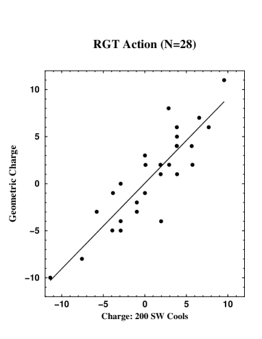
Figure 2: Comparison of geometric and cooled topological charges for RGT action lattices at $a\approx 0.1{\rm fm}$.

3 Results

As described above, we compute $Q_{p}$, $Q_{g}$, and $Q_{c}$ on all of our lattices. We show two scatter plots (Figures 1, 2) highlighting the discrepancy between $Q_{g}$ and $Q_{c}$. The best fit line is constructed through the points on a scatter plot. The slope of this line is an estimate of the ratio of multiplicative renormalizations, and should be close to $1$ since both the geometric and cooling methods give integer charges. The correlation

$$z_{gc}=\frac{\left\langle\left(Q_{g}-\bar{Q}_{g}\right)\left(Q_{c}-\bar{Q}_{c}\right)\right\rangle}{\sqrt{\left\langle\left(Q_{g}-\bar{Q}_{g}\right)^{2}\right\rangle\left\langle\left(Q_{c}-\bar{Q}_{c}\right)^{2}\right\rangle}}$$

between $Q_{g}$ and $Q_{c}$ is a measure of random additive artifacts seen by one method but not the other, such as dislocations which disappear during cooling therefore contributing only to $Q_{g}$ but not to $Q_{c}$. The scatter plots show a strong correlation between $Q_{g}$ and $Q_{c}$ for the RGT action, and a far weaker correlation for the WA, suggesting that the effect of lattice artifacts on topological charge is far less pronounced for the improved action.

Figure 3: Correlation $z_{gc}$ between geometric and cooled topological charges, for WA, SW, and RGT ensembles. Results for three different cooling methods are shown.

Figure 4: Statistical correlation $z_{pc}$ between plaquette and cooled topological charges, for same ensembles, three cooling methods.

Table 1: Correlations, SW Cooling Linear Fits

Corr.	WA	SW, $4.2$	SW, $4.43$	RGT
$z_{gc}$	$0.28(13)$	$0.77(8)$	$0.80(6)$	$0.88(5)$
$z_{pc}$	$0.04(16)$	$0.29(16)$	$0.31(13)$	$0.32(16)$

In Fig. 3 we show a comparison between the WA, SW, and RGT actions of the correlation between $Q_{g}$ and $Q_{c}$. Fig. 4 similarly shows the correlation between $Q_{p}$ and $Q_{c}$, computed in the same manner as $z_{gc}$, and numerical values are in Table 1. The SW action serves as an intermediate point between the other two actions, since the RGT action represents a better estimate of the renormalization trajectory than the WA and SW actions. It is unclear whether the spread in $z_{gc}$ at $\beta=4.43$ is due to any systematic effect of the cooling algorithm. It is possible that for better improved actions, where the exponential suppression of dislocations is greater than for the S-W action, increasing beta will have a more profound effect than we have seen here for the S-W action. For the plaquette method, we have shown previously[6] that the multiplicative $Z_{P}$ becomes less severe as the action improves, and the increased correlation $z_{pc}$ suggests that the additive renormalization also decreases. In addition, improving the action is far more effective than increasing $\beta$ for suppressing lattice artifacts.

Future calculations can include a more comprehensive study of other improved actions. Other methods for $\chi_{t}$, including the fermionic method[7], and an indirect measurement by calculating the $\eta^{\prime}$ mass[8, 9], should also be tested. Having established a correlation between cooled and uncooled topology and located individual instantons, we are now prepared to investigate Shuryak’s picture of a dilute instanton gas, and the influence of instantons on hadronic physics by working directly on uncooled lattices.

Acknowledgement. The calculations were performed at the Ohio (OSC) and National Energy Research (NERSC) supercomputer centers, and the Advanced Computing Laboratory.

References

- [1] Gupta, Patel, Phys.Lett. B183, 193 (1987).
- [2] Cella, Phys. Lett. B333, 457 (1994).
- [3] Christou, Phys.Rev. D53, 2619 (1996).
- [4] Lüscher, Comm.Math.Phys.85, 39 (1982).
- [5] Göckeler, Phys.Lett.B233, 192 (1989).
- [6] Grandy, J. and R. Gupta, Nucl. Phys. B (Proc. Suppl.) 42, 246 (1995).
- [7] Smit & Vink, Phys.Lett. B194, 433 (1987).
- [8] Kuramashi, Phys.Rev.Lett. 72, 3448 (1994).
- [9] Kilcup, Nucl. Phys. B (Proc. Suppl.) 47, 358 (1996).