The Staggered $\eta^{\prime}$ with Smeared Operators

Abstract

We present a refined calculation of the $\eta^{\prime}$ mass using staggered fermions and Wuppertal smeared operators to suppress excited state contributions. We use quenched and dynamical configurations of size $16^{3}\times 32$, with $N_{f}=0$, $N_{f}=2$ and $N_{f}=4$, and compare our results with the expected theoretical forms from quenched, partially quenched, and unquenched chiral perturbation theory.

1 INTRODUCTION

The pseudoscalar spectrum of QCD consists of an octet of mesons which are approximate Goldstone bosons of spontaneously broken $SU(3)$ axial flavor symmetry, plus an anomalously heavy flavor singlet meson, the $\eta^{\prime}$. The heaviness of the $\eta^{\prime}$ is attributed to the effects of topology [1]. In an $SU(3)$ symmetric world, $m_{\eta^{\prime}}$ would obey

$$m_{\eta^{\prime}}^{2}=m_{0}^{2}+m_{8}^{2}$$ (1)

where $m_{8}^{2}$ is the average mass squared of the octet mesons which vanishes in the chiral limit, while $m_{0}^{2}$ is the topological contribution which does not vanish in the chiral limit. Neglecting $\eta$-$\eta^{\prime}$ mixing, one plugs in the known meson masses to obtain the “experimental” value $m_{0}(N_{f}=3)=860{\rm MeV}$.

2 LATTICE CALCULATION OF $m_{\eta^{\prime}}$

Extraction of $m_{\eta^{\prime}}$ from first principles has received much attention [2, 3, 4, 5]. The focus in all these studies has been to calculate the ratio $R(t)$ defined below

$$R(t)=\frac{\langle\eta^{\prime}(t)\eta^{\prime}(0){\rangle}_{2-loop}}{\langle\eta^{\prime}(t)\eta^{\prime}(0){\rangle}_{1-loop}}$$ (2)

where $\eta^{\prime}(t)$ is the operator that creates or destroys an $\eta^{\prime}$ meson (in terms of quark fields, for staggered fermions, this becomes $\overline{Q}{\gamma}_{5}\otimes IQ$). Two point correlation function of this operator yields both a disconnected diagram (referred to as 2-loop in eqn 2) and a connected diagram (1-loop).

On dynamical configurations, when $m_{val}=m_{dyn}$, $R(t)$ takes the following asymptotic form

$$R(t)=\frac{N_{v}}{N_{f}}\,\,[1\,\,-\,\,B\exp(-\Delta mt)]$$ (3)

where $N_{v}$ is the number of valence fermions, $N_{f}$ is the number of dynamical fermions, B is a constant and $\Delta m=m_{\eta^{\prime}}-m_{8}$.

For the quenched configurations, infinite iteration of the basic double pole vertex does not exist and it can be shown that the ratio is a linear function of time [2].

$$R(t)=const.+\frac{m_{0}^{2}}{2m_{8}}\,t$$ (4)

This style of calculation was employed by the authors of [2] who obtained a result of $m_{0}(N_{f}=3)=751(39){\rm MeV}$ using quenched configurations and Wilson fermions. We used staggered fermions and both dynamical and quenched configurations and reported a value of $m_{0}(N_{f}=3)=730(250){\rm MeV}$ extracted from dynamical configurations in [3].

3 SIMULATION DETAILS

The parameters of the ensemble used in the simulation are shown in table 1. For all of the configurations listed in table 1 the inverse lattice spacing is about 2 GeV as obtained from $m_{\rho}$ [7]. $m_{val}$ for the quenched configurations has been chosen 10% higher than that corresponding to dynamical ($m_{dyn}=0.01$, $N_{f}=2$) so that $m_{8}$ is same for both. Propagators were computed using conjugate gradient on the 128 node OSC Cray T3D machine. For details concerning performance, the type of source, the method adopted for calculating the disconnected propagator etc., the reader is referred to  [3].

Table 1: The Statistical Ensemble

$N_{f}$	$m_{dyn}$	$\beta$	$N_{samp}$	$m_{val}$
0	$\infty$	6.0	83	0.011
				0.022
				0.033
2	0.01	5.7	79	0.01
				0.02
				0.03
2	0.015	5.7	50	0.01
				0.015
2	0.025	5.7	34	0.01
				0.025
4	0.01	5.4	70	0.01

3.1 Smearing

The disconnected data is noisy and clean signals exist only for the first few time slices. Smearing helps in reducing excited state contributions from the first few time slices, thus enabling a reliable extraction of $\Delta m$. We use the gauge invariant Wuppertal smearing technique.

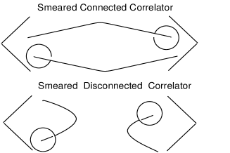
Figure 1: Correlators from Smeared Operators

For the connected contraction we computed two propagators, one with a smeared source and point-like sink and the other with a point-like source and smeared sink (see Fig. 1). Correspondingly, for the disconnected loops, the sink end was smeared in the same way(SS).

Figure 2: Ratio from SS and LL correlators at $m_{val}=m_{dyn}=0.01$

Fig. 2 compares the ratio plot with and without smearing on dynamical configurations. In the initial few time slices both the data are different but they begin to coincide after a few time slices as they should.

4 RESULTS

Fig. 3 shows the form of the ratio on all the configurations listed in Table 1. For $N_{f}=2$ and $N_{f}=4$, the points shown are for $m_{val}=m_{dyn}$, while for $N_{f}=0$ we plot $m_{val}=0.011$. It is gratifying to see that this observable clearly distinguishes the number of flavors.

Figure 3: $N_{f}$ dependence of ratio

One extracts $m_{0}^{2}$ from a linear fit to the quenched data. Fig. 4 shows $m_{0}^{2}$ versus $m_{val}$ obtained from both local and the smeared data, fit linearly and extrapolated to the chiral limit. As is expected, $m_{0}^{2}$ does not vanish in the chiral limit.

Figure 4: Chiral extrapolation of $m_{0}^{2}$

The $N_{f}=2$ data shown in Fig. 3 is fit to the form of eqn 3. From the fit one extracts $\Delta m$ and hence $m_{\eta^{\prime}}$ for all the values of $m_{dyn}$ shown. It can be seen in Fig. 5 that $m_{\eta^{\prime}}$ does not vanish in the chiral limit.

Figure 5: Chiral extrapolation of $m_{\eta^{\prime}}^{2}$

When $m_{val}\neq m_{dyn}$, the ratio $R(t)$ takes the form

$$R(t)=\,\,\frac{N_{v}}{N_{f}}\,[\,At\,\,-\,\,B\exp(-\Delta mt)\,\,+\,\,C]$$ (5)

Our data are not precise enough to allow a four parameter fit, but using lowest order $PQ\chi PT$ (and neglecting the small momentum dependent self-interaction $\alpha$) we can express $A$, $B$ and $C$ in terms of one unknown parameter, $m_{0}^{2}$. For $m_{val}>m_{dyn}$ ($N_{f}=2,m_{dyn}=0.01$) data we get reasonable fits and find a partially quenched result of $m_{\eta^{\prime}}(N_{f}=3)=876\pm 16$ MeV, remarkably consistent with the fully quenched and fully dynamical data. For $m_{val}\leq m_{dyn}$ the $\chi^{2}$ is not reasonable. On the other hand, one need not venture far from lowest order $PQ\chi PT$ to fit the data. For example, from two parameter fits to the dynamical data, one obtains $Z^{\prime}/Z$, the ratio of the residues for creating $\eta$ and $\eta^{\prime}$. While this ratio is set to unity at lowest order, the data prefer values 20-30% larger, an amount which could easily be accommodated by higher order chiral and $O(1/N_{c})$ corrections.

Figure 6: $Z^{\prime}/Z$ versus $m_{dyn}$

5 CONCLUSIONS

The value, we obtain for $m_{\eta^{\prime}}$ in the chiral limit are summarized in the table below. Smeared operators have produced a lower value for $m_{\eta^{\prime}}$ than that obtained from local operators.

Table 2: $m_{\eta^{\prime}}(N_{f}=3)$ in the chiral limit

	Quenched	Dynamical ($m_{dyn}=m_{val}$)
	(MeV)	(MeV)
LL	1156(95)	974(133)
SS	891(101)	780(187)

Within the quoted statistical errors, the values obtained above are consistent with experiment.

References

- [1] E. Witten, Nucl. Phys. B156 (1979) 269.
- [2] Y. Kuramashi et al., Phys. Rev. Lett. 72 (1994) 3448.
- [3] G. Kilcup et al., Proceedings of Lattice ’95.
- [4] M. Masetti et al., these proceedings.
- [5] H. Thacker et al., these proceedings.
- [6] C. Bernard and M. Golterman Phys. Rev. D49 (1994) 486-494
- [7] D. Chen et al., these proceedings.