Dynamical Fermion on Random-Block Lattice

Abstract

Massless fermion field interacting with abelian dynamical gauge field on 2-dimensional random-block lattices are investigated using Hybrid Monte Carlo simulations. Preliminary results of the Wilson loop and the chiral correlation function are in agreement with the continuum Schwinger model.

1 INTRODUCTION

The problem of formulating the chiral fermion field on space-time lattices has been discussed from the viewpoint of funtional integrals [1]. I argued that the functional integral measure provided by any $single$ lattice ( hypercubical lattice or random lattice ) is not sufficent to yield fermionic functional integrals to agree with the continuum field theory. My proposal of using an ensemble of random-block lattices ( RBL ) to provide a proper measure has been investigated. RBL regularization has been tested for the free fermion ( massive and massless ) in $2d$ and $4d$ [2, 3] respectively, and for $2d$ massless fermion in an external abelian gauge field [4, 5]. All observables including fermion propagators, gauge invariant currents, axial anomaly and current-current correlations are all in good agreement with the continuum field theory. It is natural for us to proceed to investigations involving dynamical fermion field on RBL. In this paper, massless fermion field interacting with the dynamical abelian gauge field on 2d RBL is studied. Using Hybrid Monte Carlo simulations, the Wilson loop and the chiral correlation function are measured and preliminary results of these observables are in agreement with the continuum Schwinger model. More extensive measurements involving higher statistics and larger lattices are now in progress and will be reported elsewhere.

2 SCHWINGER MODEL on RBL

The action of a massless fermion field interacting with the dynamical abelian gauge field on a $2d$ RBL is

$$A_{rbl}=\sum_{i,\mu}\omega_{i}K_{i}^{\mu}{\bar{\psi}_{i}}\gamma_{\mu}[U_{\mu}(i)\psi_{i+\hat{\mu}}-U_{\mu}^{\dagger}(i-\hat{\mu})\psi_{i-\hat{\mu}}]$$

$$+\beta\sum_{p}w_{p}[1-{\rm Re}(U_{p})]$$

where $\psi_{i}$ and $\bar{\psi}_{i}$ are two independent 2-component spinors at site $i$, $\omega_{i}=\prod_{\mu}\frac{(x_{i+{\hat{\mu}}}-x_{i-{\hat{\mu}}})}{2}$ is the site weight at site $i$, $K_{i}^{\mu}=(x_{i+{\hat{\mu}}}-x_{i-{\hat{\mu}}})^{-1}$ is the inverse of the distance between the sites $i+\hat{\mu}$ and $i-\hat{\mu}$ and $U_{\mu}(i)=\exp[{\rm ie}\int_{x_{i}}^{x_{i+\mu}}\vec{A}\cdot\vec{dl}]$ is the link variable pointing from the site $i$ to the site $i+\hat{\mu}$, and the $\gamma$ matrices are chosen to be $\gamma_{1}=\sigma_{1}$, $\gamma_{2}=\sigma_{2}$ and $\gamma_{5}=-i\gamma_{1}\gamma_{2}=\sigma_{3}$. The last term in the action $A_{rbl}$ is due to the pure gauge field and is conveniently labeled as

$$A_{g}[U]=\beta\sum_{p}w_{p}[1-{\rm Re}(U_{p})]$$

where $\beta=\frac{1}{e^{2}}$, $U_{p}$ is the path-ordered product of the link variables around a plaquette $p$, $w_{p}=\frac{1}{S_{p}}$ is the weight of the plaquette $p$ and $S_{p}$ the area of the plaquette. The action $A_{rbl}$ is invariant under the $U_{V}(1)$ transformation

$$\psi_{i} \rightarrow \exp({\rm-ie}\theta_{i})\psi_{i}$$

$$\bar{\psi}_{i} \rightarrow \bar{\psi}_{i}\exp({\rm ie}\theta_{i})$$

$$U_{\mu}(i) \rightarrow \exp({\rm-ie}\theta_{i})U_{\mu}(i)\exp({\rm ie}\theta_{i+\hat{\mu}})$$

and the $U_{A}(1)$ transformation

$$\psi_{i} \rightarrow \exp({\rm ie}\gamma_{5}\alpha)\psi_{i}$$

$$\bar{\psi}_{i} \rightarrow \bar{\psi}_{i}\exp({\rm ie}\gamma_{5}\alpha)$$

where $\alpha$ is a global parameter. In the continuum limit, $A_{rbl}$ goes to the Schwinger model [6]

$$A_{S}=\int d^{2}x\left({\bar{\psi}}(x)\gamma_{\mu}[\partial_{\mu}+{\rm ie}A_{\mu}(x)]\psi(x)+\frac{1}{4}F_{\mu\nu}^{2}\right)$$

The partition function of $A_{rbl}$ is

$$Z = \int[dU][d\psi][d\bar{\psi}]\exp(-A_{rbl})$$

$$= \int[dU]det(G)\exp(-A_{g}[U])$$

where $G$ is the matrix

$$G_{ij}^{\alpha\beta}=\gamma_{\mu}^{\alpha\beta}\omega_{i}K_{i}^{\mu}[U_{\mu}(i)\delta_{j,i+\hat{\mu}}-U_{\mu}^{\dagger}(i-\hat{\mu})\delta_{j,i-\hat{\mu}}]$$

and $det(G)$ is positive definite even for one single flavor of the fermion field . With $\gamma_{1}=\sigma_{1}$, $\gamma_{2}=\sigma_{2}$, $G$ can be written as

$$G=\left(\begin{array}[]{cc}0&T_{1}-iT_{2}\\ T_{1}+iT_{2}&0\end{array}\right)$$

where $T_{1}$ and $T_{2}$ are anti-hermitian matrices, $T_{1}^{\dagger}=-T_{1}$ and $T_{2}^{\dagger}=-T_{2}$. Then

$$G = \left(\begin{array}[]{cc}0&-(T_{1}+iT_{2})^{\dagger}\\ T_{1}+iT_{2}&0\end{array}\right)$$

and

$$\det G = \det(T_{1}+iT_{2})\cdot\det(T_{1}+iT_{2})^{\dagger}(-1)^{n_{s}}$$

$$= \left|\det(T_{1}+iT_{2})\right|^{2}$$

$$\equiv \det(K^{\dagger}K)>0$$

where $K\equiv T_{1}+iT_{2}$ and $n_{s}$ is the total number of sites which is assumed to be even. Therefore the probability distribution function is positive definite for any gauge configurations and thus amenable for Monte Carlo simulations. Complex scalar fields {$\phi_{i},\phi_{i}^{*}$} are introduced to convert $det(G)$ to a functional integral over the complex scalar fields. The partition function becomes

$$Z\simeq\int[dU][d\phi^{\dagger}][d\phi]\exp\left(-A_{g}[U]-\phi^{\dagger}(K^{\dagger}K)^{-1}\phi\right)$$

$$\simeq\int[dU][d\xi^{\dagger}][d\xi]\exp\left(-A_{g}[U]-\xi^{\dagger}\xi\right)$$

where $\xi\equiv(K^{\dagger})^{-1}\phi$. Then the system is equivalent to that of effective action $A_{eff}=A_{g}[U]+\xi^{\dagger}\xi$ in which quantum expectation value of any observables can be computed by the Hybrid Monte Carlo ( HMC ) simulation [7]. The procedures of performing the HMC simulation are similar to those on a hypercubical lattice.

3 OBSERVABLES

Measurements of the Wilson loop and the chiral correlation function at $\beta=10.0$ were performed using an ensemble of $64$ random-block lattices each of size $12\times 12$ and average lattice spacing $a=1.0$. On each RBL, $2000$ sweeps are used for thermalization, $1000$ measurements were performed with consecutive measurements separated by $10$ sweeps. More extensive measurements with higher statistics and on larger lattices are now in progress and will be presented elsewhere.

CHIRAL CORRELATION FUNCTION

One remarkable feature of the continuum Schwinger model is that all gauge-invariant quantities can be computed exactly. The most interesting physics of the model is that the chiral symmetry is dynamically broken by quantum corrections. This can be observed in the chiral correlation function

$$C(x,y)\equiv<\bar{\psi}(x)\frac{1+\gamma_{5}}{2}\psi(x)\bar{\psi}(y)\frac{1-\gamma_{5}}{2}\psi(y)>$$

which goes to a non-vanishing constant for large $|x-y|$, directly indicating the breakdown of clustering and degenerate vacua in the theory. In a finite square of size $L\times L$, $C(x,y)$ can be evaluated in the following.

$$C(x,y)=\left[\sum_{\mu}S_{\mu}^{2}(x,y)\right]\times$$

$$\exp[4\pi(\Delta_{0}(x,x)-\Delta(x,x)-\Delta_{0}(x,y)+\Delta(x,y))]$$

where $S_{\mu}(x,y)$ are components of the massless fermion propagator, $\Delta_{0}(x,y)$ is the massless scalar propagator and $\Delta(x,y)$ is the massive scalar propagator with mass $\sqrt{\frac{{\rm e}^{2}}{\pi}}$. They can be expressed in the following.

$$S_{F}(x,y)=\gamma_{\mu}S_{\mu}(x,y)=\gamma_{\mu}\partial_{\mu}\Delta_{F}(x,y)$$

where

$$\Delta_{F}(x,y)=\frac{1}{L^{2}}\sum_{n_{1},n_{2}=-\infty}^{\infty}\frac{\exp[i\pi(\frac{2\vec{n}+1}{L})\cdot(\vec{x}-\vec{y})]}{[\frac{(2n_{1}+1)\pi}{L}]^{2}+[\frac{(2n_{2}+1)\pi}{L}]^{2}}$$

$$\Delta_{0}(x,y)=\frac{1}{L^{2}}\sum_{n_{1},n2=-\infty}^{\infty}\frac{\exp[i\ \frac{2\pi}{L}\vec{n}\cdot(\vec{x}-\vec{y})]}{(\frac{2n_{1}\pi}{L})^{2}+(\frac{2n_{2}\pi}{L})^{2}}$$

$$\Delta(x,y)=\frac{1}{L^{2}}\sum_{n_{1},n_{2}=-\infty}^{\infty}\frac{\exp[i\frac{2\pi}{L}\vec{n}\cdot(\vec{x}-\vec{y})]}{(\frac{2n_{1}\pi}{L})^{2}+(\frac{2n_{2}\pi}{L})^{2}+\frac{{\rm e}^{2}}{\pi}}$$

On a RBL, the chiral correlation function can be measured as

$$C_{l}(x,y)=\frac{1}{Z}\int[dU]\ det(G)\ \exp(-A_{g}[U])\times$$

$$\qquad\qquad{\rm(-1)Tr}[G^{-1}(x,y)\frac{1-\gamma_{5}}{2}G^{-1}(y,x)\frac{1+\gamma_{5}}{2}]$$

$$=\frac{1}{Z}\int[dU][d\xi][d\xi^{\dagger}]|K^{-1}(x,y)|^{2}\exp(-A_{g}[U]-\xi^{\dagger}\xi)$$

where $K^{-1}(x,y)$ is the right-handed fermion propagator in background gauge field and complex scalar field, which can be computed in the following.

$$K_{ij}^{-1}=[(K^{\dagger})^{-1}K^{\dagger}K]_{ij}^{-1}=Q_{il}^{-1}K_{lj}^{\dagger}$$

where $Q\equiv K^{\dagger}K$ and the last step is computed by the conjugate gradient method. The ensemble average is obtained by repeating the same calculation for each RBL while holding the end-points $x$ and $y$ fixed in all RBL,

$$<C(x,y)>=\frac{1}{V^{N_{s}-2}}\int\prod_{i=1}^{N_{s}}d^{2}z_{i}$$

$$\qquad\qquad\qquad\qquad\qquad\delta(z_{1}-x)\delta(z_{2}-y)C(x,y)$$

$$\simeq\frac{1}{N_{latt}}\sum_{l=1}^{N_{latt}}C_{l}(x,y)$$

This RBL regularized chiral correlation function $<C(x,y)>$ is then compared to the continuum result. In Fig. 1, $<C(x,y)>$ is plotted for an ensemble of 64 RBL each of size $12\times 12$ and average lattice spacing $a=1.0$. It agrees with the continuum Schwinger model and goes to a non-vanishing constant at large $|x-y|$.

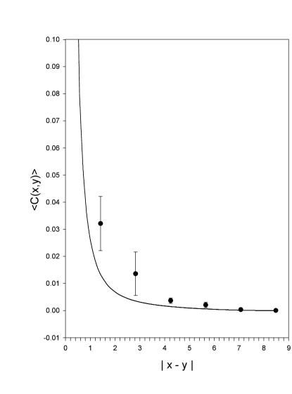
Figure 1: The chiral correlation function  $<~{}C~{}(x,y)~{}>$ plotted vs. $|x-y|$ at $\beta=10.0$. The solid line corresponds to the continuum Schwinger model.

WILSON LOOP

The chiral symmetry breaking in the Schwinger model results in complete screening of the linear confinement potential of external charges in the pure gauge theory, and the quantum expectation of the Wilson loop $W(C)=\exp\left(i{\rm e}\oint_{C}\vec{A}\cdot d\vec{x}\right)$ would display asymptotically perimeter law rather than the area law. In continuum,

$$<W(C)>=\exp\left[-\frac{{\rm e}^{2}}{4\pi}\oint_{C}\oint_{C}dx_{\mu}dy^{\mu}K_{0}(m|x-y|)\right]$$

where $m=\sqrt{\frac{{\rm e}^{2}}{\pi}}$. On a RBL, the Wilson loop can be measured as

$$W(C)_{l}=\frac{\int[dU][d\psi][d\bar{\psi}]W(C)\exp(-A_{rbl})}{\int[dU][d\psi][d\bar{\psi}]\exp(-A_{rbl})}$$

$$=\frac{\int[dU][d\xi][d\xi^{\dagger}]W(C)\exp(-A_{g}[U]-\xi^{\dagger}\xi)}{\int[dU][d\xi][d\xi^{\dagger}]\exp(-A_{g}[U]-\xi^{\dagger}\xi)}$$

The ensemble average can be obtained by repeating the same calculation for each RBL while holding the boundary of the Wilson loop fixed in all RBL. For a square Wilson loop of size $D\times D$, in practice, we can increase the statistics by measuring all Wilson loops having $D$ links in both directions respectively, and the average area of these Wilson loops is $D\times D$. Unlike the chiral correlation function or other observables involving fermion fields, the fluctuations of the Wilson loop from one RBL to another is rather small and the number of RBL used for ensemble averaging can be minimum. In Fig. 2, the quantum expectation values of $D\times D$ Wilson loops for an ensemble of 64 RBL are plotted vs. $D$. The values are in good agreement with the continuum Schwinger model, indicating the complete screening of the confinment potential in the pure gauge theory.

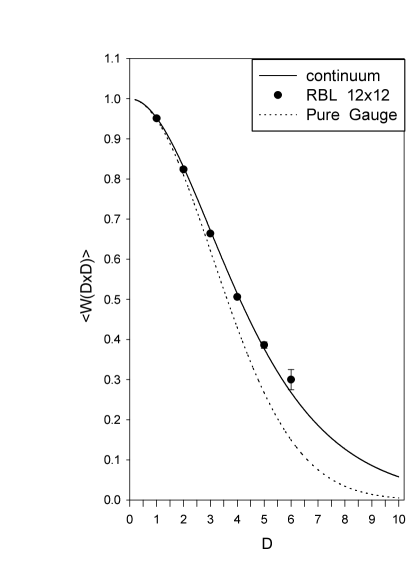
Figure 2: The values for $D\times D$ Wilson loop plotted vs. $D$ at $\beta=10.0$. The solid line corresponds to the continuum Schwinger model while the dotted line to the pure gauge theory.

4 CONCLUSIONS and DISCUSSIONS

The present investigation of the dynamical fermion field on RBL is far from completed yet. Besides the Wilson loop and the chiral correlation function, other observables must also be measured, all must be with higher statistics and on larger lattices as well as for many different $\beta$ values. These measurements are now in progress and the results will be presented elsewhere. The present preliminary results are consistent with the conclusions drawn from previous studies of free fermion and fermion in a background gauge field on RBL, that an ensemble of RBL could provide a proper measure for functional integrals involving fermion fields. Without breaking the chiral symmetry at the tree level, RBL regularization uses the naive fermion which presumably suffers from the species doubling on any one of the lattices, however miraculously gives the correct result when the functional integrals are sumed over all RBL. The most remarkable feature is that it produces the correct chiral symmetry breaking through quantum corrections. Whether RBL regularization also works for the chiral guage theories, say chiral Schwinger model or the Electroweak theory is still an open but very interesting question.

References

• [1] T.W. Chiu, Nucl. Phys. B ( Proc. Suppl.) 42 (1995) 603.
• [2] T.W. Chiu, Phys. Lett. B 206 (1988) 510.
• [3] T.W. Chiu, Phys. Lett. B 217 (1989) 151.
• [4] T.W. Chiu, ”Massless Fermion Field on 2D Random-Block Lattice”, NTUTH-93-16, September, 1993.
• [5] T.W. Chiu, Nucl. Phys. B ( Proc. Suppl.) 34 (1994) 599.
• [6] J. Schwinger, Phys. Rev. 128 (1962) 2425.
• [7] S. Duane, A.D. Kennedy, B.J. Pendleton and D. Roweth, Phys. Lett., B195 ( 1987) 216.