Approximate Actions for Lattice QCD Simulation

Abstract

We describe a systematic approach to generating approximate actions for the lattice simulation of QCD. Three different tuning conditions are defined to match approximate with true actions, and it is shown that these three conditions become equivalent when the approximate and true actions are sufficiently close. We present a detailed study of approximate actions in the lattice Schwinger model together with an exploratory study of full QCD at unphysical parameter values. We find that the technicalities of the approximate action approach work quite well. However, very delicate tuning is necessary to find an approximate action which gives good predictions for all physical observables. Our best view of the immediate applicability of the methods we describe is to allow high statistics studies of particular physical observables after a low statistics full fermion simulation has been used to prepare the stage.

I Introduction

The design of improved algorithms for simulation with dynamical fermions has provided an important challenge for lattice QCD. Perturbative arguments and numerical experiments suggest that a significant component of the effect of dynamical quarks can be accounted for by a shift in the effective lattice spacing. The quenched approximation takes this view to its extreme, and ignores all dynamical quark effects except for this shift in scale. In most cases, the systematic errors introduced by quenching have so far turned out to be of the same order as the best presently achievable statistical errors in full dynamical simulations. As available computer power grows, and as we study larger volumes and smaller lattice spacings, we can expect this situation to change, and to begin to see significant discrepancies between quenched and full theory results. Systematic errors due to quenching will then turn out be larger than full theory statistical errors, and the quenched approximation will loose its usefulness.

In a recent paper [1] it has been shown that the quenched algorithm is a single member of a large class of approximate QCD simulation algorithms. The members of this class interpolate in a smooth fashion between the extreme cases of quenched QCD simulations on the one hand, and full dynamical QCD simulations on the other. Individual members can be considered as different approximations to the full dynamical QCD action. So long as the quenched approximation represents the only significant example of an approximate simulation algorithm, it is possible to consider it in isolation and to accept its historically important contributions to lattice QCD while remaining wary of its mathematical correctness. However, once one begins to consider variants which seek to improve on the quenched approximation without themselves being exact, a number of important issues arise, and a more critical approach is needed.

First, of course, is the question of what we mean mathematically by the term ‘approximate action’. The qualitative view of quenched QCD which we normally adopt is that, at fixed lattice spacing and coupling, it produces ensembles which are reasonably close to the ensembles which would be generated for full QCD at some shifted coupling. Reasonable closeness is however a vague term. What it tends to mean in practice is that ensemble expectations of a set of operators in quenched and full QCD seem to agree within statistical errors, so long as one allows for an effective lattice spacing shift.

In this paper we consider the general principles which can be applied to define what is meant by a simulation algorithm based on an approximate action in the sense defined by the quenched approximation. We will describe a systematic approach to generating approximate actions and will discuss conditions which allow the tuning of any candidate approximate action to optimize its matching to a true action of interest. The methods we develop, while motivated by the approximate action view, are also applicable whenever we wish to match results from different lattice simulations. In particular, the tuning we propose defines the optimum matching conditions between Wilson and Kogut-Susskind fermion simulations, and between naive and improved action simulations.

A second issue of concern, when considering simulations with approximate actions, is the question of their computational performance. The results reported in [1] were obtained on very small systems, and for these systems it was found that approximate action simulations were very competitive with exact simulations including full fermions. However, a question left unanswered was whether this competitiveness would continue when the method was applied to more realistic situations. The basic proposal of [1] was to attempt an approximation of the fermion determinant in QCD using Wilson loop operators of increasing size. On a small system there are relatively few such operators, but the number of operators grows very fast as the size of the system increases and the computational work required would also grow. Some preliminary data which we reported in [2] for the case of the Schwinger model seems to bear out this view. There we found that only very slow improvements in the quality of the approximation were achieved as Wilson loops of systematically increasing size were added to the approximate action. An independent study of QCD at realistic lattice sizes [3] was also somewhat negative. This study found that the plaquette operator was actually a very poor approximation to the fermion determinant in typical large simulation. Both of these results suggest that very many Wilson loops would be needed to get a numerically useful approximation in realistic situations.

We report in this paper, however, that the pessimistic view just described is an artifact of the particular approximation prescription defined in [1]. The systematic approach to tuning approximate actions which we develop here allows us to generate much more aggressive approximations than are otherwise possible, and we find that it is not necessary to include Wilson loops of all shapes and sizes to get useful approximate actions. Indeed, the best approximate actions in the Schwinger model and QCD cases which we have studied are found to include only a few Wilson loop operators of quite surprising shape and dimension.

An issue which we do not address in this paper is that of the behaviour of approximate actions in the continuum limit. The quenched case is clearly problematic in this limit [4]. However, the strategy we propose here is a numerical one in which one may choose the most appropriate approximate action for any given simulation at fixed lattice spacing and coupling. If one varies the lattice spacing and coupling, then the corresponding approximate action would also vary. It seems conceivable to us that the variations in approximate action which result would be sufficient to allow a mathematically correct continuum limit of the approximate action to be taken.

The plan of the remainder of this paper is as follows. In Section II, we define a simple cumulant expansion method which allows direct comparison of the expectations of operators calculated in two different path integral measures. We argue that this expansion method is the most efficient way of determining the shifts introduced in expectations of physical observables due to changes in the underlying path integral measure.

The concept of an approximate action is defined in Section III. The quenched QCD action is the prototypical example here. Approximate actions allow us to define corresponding approximate simulation algorithms, and we develop in this section three different ways in which approximate actions might be defined. We then argue that all three definitions become equivalent when the approximate action is sufficiently close to the action which it attempts to approximate.

As an initial test, we consider the Schwinger model. Section IV gives the explicit form of this two-dimensional model which we have used, and describes some necessary technical features of the calculations. Simulation results are presented in the following two sections. In Section V, we consider the quenched approximation in some detail. Physical quantities calculated here include the static potential and the mass of the mesonic bound state of the model. We present comparisons of these observables calculated in the quenched approximate simulation and full dynamical simulation. Section VI describes a variety of different extensions to the quenched approximation. The analysis begins with the scenario proposed in [1] in which the fermion determinant is expanded in terms of Wilson loops of increasing size. We show first that this expansion technique is quite straightforward to execute and appears to be numerically stable. We argue, however, that this ordered expansion is very slow to converge. Instead, we propose an aggressive approach to developing approximate actions which directly targets the interesting physics. This approach is seen to improve considerably the slow convergence apparent in [1].

In Section VII, we describe a trial application of the approximate action approach to QCD. The purpose of the test is to gain some understanding of the potential of the method for QCD simulation and to identify practical problems which remain to be solved. The test described is for a small lattice with heavy quarks.

Finally, our conclusions are presented in Section VIII.

II The Comparison of Path Integral Measures

In all lattice simulation, the goal is to calculate expectation values of interesting operators in some path integral measure. The measure is given by some action which we think of as the true action and denote by $S_{t}$. Our goal is to find an action $S_{a}$ which allows us to approximate the measure generated by $S_{t}$. The prototypical example is given by lattice QCD. The fundamental degrees of freedom here are the $SU(3)$ link matrices $U_{\mu}(x)$ assigned to edges which join nearest neighbouring sites on a four dimensional hypercube. A possible ‘true’ action for this system is the lattice QCD action which includes a Wilson fermion determinant term,

$$S_{t}=-\beta\sum_{\Box}\frac{1}{3}{\rm Re}{\rm Tr}{U_{\Box}}-{\rm Tr}\log M_{\kappa}^{\dagger}M_{\kappa}$$ (1)

while a possible approximate action is the quenched lattice QCD action,

$$S_{a}=-\beta^{\prime}\sum_{\Box}\frac{1}{3}{\rm Re}{\rm Tr}{U_{\Box}}\,.$$ (2)

$U_{\Box}$ here represents the product of gauge links around a fundamental plaquette, while $M_{\kappa}$ is the Wilson fermion matrix for hopping parameter $\kappa$. We have also implicitly allowed for a bare coupling shift between exact and approximate cases by including different $\beta$’s in the different actions.

Expectation values of operators $F$ in the path integral measures generated by $S_{t}$ and $S_{a}$ are denoted respectively by $\langle F\rangle_{t}$ and $\langle F\rangle_{a}$, and are given by

$$\langle F\rangle_{t}=\frac{\int{[dU]\;{F}\;e^{-S_{t}}}}{\int{[dU]\;e^{-S_{t}}}}\quad\text{and}\quad\langle F\rangle_{a}=\frac{\int{[dU]\;{F}\;e^{-S_{a}}}}{\int{[dU]\;e^{-S_{a}}}}\,.$$ (3)

Before addressing the problem of how to choose an approximate action, we first need a technique to compare these expectations. The simplest numerical comparison technique is to generate independent sequences of configurations for each measure, to evaluate expectations on these sequences, and then compare. For our purposes, this simple approach is not computationally feasible. We are attempting to find approximate actions for a given true action because the computational work needed to generate independent configurations in the true measure is very large. Our eventual goal is to find a tuning technique which allows us to generate an approximate action without ever having to simulate the measure of the true action. Thus we are lead to consider methods by which we can use ensembles of configurations generated in one measure to estimate expectations of operators in a second measure.

Provided the fundamental degrees of freedom of two action functionals, $S_{1}$ and $S_{2}$, are the same (i.e. provided the configuration space upon which they are defined is the same), we can directly relate expectations in the corresponding measures,

$$\langle F\rangle_{j}=\frac{\langle Fe^{S_{i}-S_{j}}\rangle_{i}}{\langle e^{S_{i}-S_{j}}\rangle_{i}}=\langle F\rangle_{i}+\langle\left(F-\langle F\rangle_{i}\right)C_{i}(\Delta_{ij})\rangle_{i}\,,$$ (4)

where

$$\Delta_{ij}=S_{i}-S_{j}=-\Delta_{ji}$$ (5)

and

$$C_{i}(\Delta)=\frac{1}{\langle e^{\Delta}\rangle_{i}}e^{\Delta}\,.$$ (6)

This comparison formula is exact. However, the calculation of the overlap expectations of $C_{i}(\Delta_{ij})$ with $F-\langle F\rangle_{i}$ is very difficult numerically, since $\Delta_{ij}$ is typically a quantity which is of $O(V)$, where $V$ is the volume of our system. If we use this formula, therefore, to calculate expectations for $S_{j}$ by correcting an ensemble of configurations generated for $S_{i}$, we find that we must re-weight with factors which are $O(e^{V})$. The fluctuations in expectations so calculated are also of $O(e^{V})$, so the work needed to get reasonable statistics is exponential in $V$. As a result, a direct application of this formula to compare $\langle F\rangle_{i}$ and $\langle F\rangle_{j}$ is not feasible numerically.

We adopt instead a cumulant expansion technique which is generated by expanding $C_{i}(\Delta)$ in a Taylor series,

$$C_{i}(\Delta) = 1+\left(\Delta-\langle\Delta\rangle_{i}\right)$$ (8)

$$+\frac{1}{2}\left(\left(\Delta-\langle\Delta\rangle_{i}\right)^{2}+\langle\Delta\rangle_{i}^{2}-\langle\Delta^{2}\rangle_{i}\right)+\cdots.$$

Substituting this expansion in (4), we find

$$\langle F\rangle_{j}-\langle F\rangle_{i} = \langle\left(F-\langle F\rangle_{i}\right)\left(\Delta_{ij}-\langle\Delta_{ij}\rangle_{i}\right)\rangle_{i}$$ (10)

$$+\frac{1}{2}\langle\left(F-\langle F\rangle_{i}\right)\left(\Delta_{ij}-\langle\Delta_{ij}\rangle_{i}\right)^{2}\rangle_{i}+\cdots.$$

The leading term on the right hand side here is the connected part of the correlation of the operator $F$ with the difference in the actions $\Delta_{ij}$. As before, $\Delta_{ij}$ is a quantity of $O(V)$; but now we don’t have to exponentiate, and so we expect fluctuations only of $O(V)$ rather than $O(e^{V})$. Since any numerical simulation must be carried out at finite volume, we can expect that at least this leading correction between the expectation values in the different measures will be calculable with finite work. Of course, higher order terms will require calculation of connected correlations involving higher powers of $\Delta_{ij}$. These correlations will have correspondingly larger fluctuations. The connected correlations involving $\Delta_{ij}^{n}$ will have fluctuations of $O(V^{n})$, for example, and will be correspondingly harder to calculate. One should view this cumulant expansion technique, therefore, as the numerical version of an asymptotic expansion. If the difference $\Delta_{ij}$ is sufficiently small, one or perhaps two terms in this expansion may be calculable with reasonable work.

III Tuning the Approximate Action

In our prototypical example introduced in the last section, the true action $S_{t}$ is the lattice QCD action which combines a single plaquette gauge term and a Wilson fermion determinant term expressed as the trace of the log of the Wilson hopping matrix. Our prototypical approximate action $S_{a}$ includes just the single plaquette gauge term but with a possibly different coupling from that in the true action. More generally, we imagine that the approximate action depends on a finite number of couplings $a_{1},\ldots,a_{n}$,

$$S_{a}\equiv S_{a}(a_{1},\ldots,a_{n})\,.$$ (12)

One possibility, for example, is that $S_{a}$ includes a sum of different translationally invariant Wilson loop operators [1]. The $a_{i}$ are then the couplings multiplying each different Wilson loop operator in the sum. Another possibility is to replace the fermion determinant term with an approximate bosonic term proposed by Lüscher [5]. The $a_{i}$ then include the plaquette coupling for the gauge term together with all the roots of the polynomial used to approximate the inverse of the fermion matrix in the Lüscher approach. The question we now address is how to choose the couplings $a_{i}$ so that $S_{a}$ becomes a good approximation to the true action $S_{t}$. We define three different tuning schemes for the coefficients, and show that these three different schemes are closely related.

A Minimizing the Distance Norm

The first tuning procedure is described in [1]. There it is observed that the measure defined by an action functional $S$ allows us to define an inner product $(\,,\,)$ on the space of gauge invariant functionals of the link matrices, which takes the form,

$$(F,G)=\langle F^{*}G\rangle=\frac{\int{[dU]\;{F^{*}G}\;e^{-S}}}{\int{[dU]\;e^{-S}}}\,,$$ (13)

where $F$, $G$, and $S$ are all functions of the link matrices $U_{\mu}(x)$. This inner product turns the space of gauge invariant functions into a Hilbert space, and allows us to define the distance $d(F,G)$ between any two functions as

$$d(F,G)=((F-G),(F-G))=\langle(F-G)^{*}(F-G)\rangle\,.$$ (14)

Functions of link matrices can now be considered as vectors in this Hilbert space and the natural tuning condition in this language is to minimize the distance, or equivalently to maximize the overlap, between the two vectors which represent the true and approximate actions. Since an overall constant shift in an action functional has no effect on the measure it generates, the tuning should minimize the connected part only. Thus, the first prescription is to minimize

$$d(S_{a}-\langle S_{a}\rangle,S_{t}-\langle S_{t}\rangle)=\langle(\Delta_{at}-\langle\Delta_{at}\rangle)^{2}\rangle$$ (15)

over the space of couplings $a_{1},\dots,a_{n}$. $\Delta_{at}$ is the difference in the approximate and true actions,

$$\Delta_{at}=S_{a}-S_{t}=-\Delta_{ta}$$ (16)

and the object to be minimized is simply the variance $\sigma^{2}(\Delta_{at})$ of this difference,

$$\sigma^{2}(\Delta_{at})=\langle(\Delta_{at}-\langle\Delta_{at}\rangle)^{2}\rangle$$ (17)

evaluated in the measure $\langle\ \rangle$. Differentiating with respect to each of these couplings in turn, we generate a set of $n$ simultaneous equations to determine the minimum,

$$\langle({\cal S}_{i}-\langle{\cal S}_{i}\rangle)(\Delta_{at}-\langle\Delta_{at}\rangle)\rangle=0\quad\text{ for {\hbox{i = 1, \dots, n}},}$$ (18)

where

$${\cal S}_{i}=\frac{\partial}{\partial a_{i}}S_{a}(a_{1},\dots,a_{n})\,.$$ (19)

In deriving this particular tuning condition, we have been purposefully vague about the measure in which expectations are to be evaluated. There are two obvious measures available, that generated by $S_{t}$, and that generated by $S_{a}$. Either measure will allow a calculation of the tuned values for the couplings $a_{i}$, so this first tuning condition actually has two possible variants. Our preferred choice is to minimize in the true measure. This minimization is an explicit problem, but in principle requires generating a set of configurations in the full measure. In practice, we could also use the cumulative expansion methods of the last section to estimate expectations in the true measure using our best guess as to the approximate measure. Minimizing in the approximate measure, on the other hand, is an implicit problem since we only learn the correct values for the coefficients $a_{i}$ after the minimization is completed. Minimization in this case requires an iterative method which first guesses the correct couplings, then evaluates the corrections to those guesses.

For notational simplicity in what follows, we will assume that equations of the form (18) apply for all values of $i$, and we will drop the phrase ‘for $i=1,\dots,n$’ in such equations.

B Operator Matching

A different approach to tuning the approximate action is suggested by the observation that, in some cases at least, both true and approximate actions represent different regularizations of the same continuum theory. For the prototypical case of full Wilson fermion action versus quenched action this is, of course, not correct since the quenched approximate action does not have a unitary continuum limit. However, it is possible to imagine cases where this is indeed true. For example, one could consider the case where one action was the full Wilson fermion action, while the second action was an $O(a)$ improved action. In this view, the couplings in both actions are bare parameters in different regularizations of the same continuum theory.

Normally, one fixes the mapping from bare to renormalized couplings by specifying renormalization conditions for each bare parameter whose finite part needs to be fixed. These conditions directly relate regularized theories to the renormalized continuum theories which they regulate. In our case, imposing renormalization conditions which relate the regularized theories to continuum renormalized theories is not feasible, since this requires that we separately generate a full continuum limit extrapolation of each regularized theory. What one can do, however, is to impose renormalization conditions directly between the two lattice regularized theories. If these conditions are maintained in the passage to the continuum limit, then both regularized theories will proceed to the same renormalized continuum theory as we require.

Consider, therefore, matching the approximate action $S_{a}(a_{1},\ldots,a_{n})$ with the true action $S_{t}$. The approximate action has $n$ couplings which must be determined, so we must impose $n$ independent matching conditions between the approximate and true measures to fix these $n$ couplings. The obvious possibilities include matching operators such as $m_{\pi}$, $m_{\rho}$, $m_{N}$ [6]. These particular operators however are not ideal for our purposes since they are difficult to measure accurately on a small number of configurations, and they are not particularly sensitive to small changes in the couplings $a_{i}$ which we need to determine. The choice of matching conditions which we make, however, is not really very important since any set of conditions will correctly fix the cutoff dependent divergences of the couplings being matched, and will differ only in the way they fix finite parts. Different matchings will differ by finite renormalizations only, so we are free to choose some simply implemented matching conditions. An alternative set which is simple to calculate, and which should be sensitive to changes in the $a_{i}$, is to match the operators ${\cal S}_{i}=\partial S/\partial a_{i}$ between the approximate and true actions.

Thus, the second tuning condition we propose is to match the expectations of the $n$ operators ${\cal S}_{i}$ ($i=1,\dots,n$) in the approximate and true measures,

$$\langle{\cal S}_{i}\rangle_{t}=\langle{\cal S}_{i}\rangle_{a}.$$ (20)

Applying the cumulant expansion to $\langle S_{i}\rangle_{a}$, we find

$$\langle{\cal S}_{i}\rangle_{t}=\langle{\cal S}_{i}\rangle_{t}+\langle({\cal S}_{i}-\langle{\cal S}_{i}\rangle_{t})C_{t}(-\Delta_{at})\rangle_{t}\,,$$ (21)

which directly gives

$$\langle({\cal S}_{i}-\langle{\cal S}_{i}\rangle_{t})C_{t}(-\Delta_{at})\rangle_{t}=0\,.$$ (22)

C Maximizing Acceptance

Consider using an approximate action as part of an exact Markov process which generates configurations distributed according to the measure of the true action. The particular exact algorithm we propose involves a standard Markov transition step which satisfies detailed balance for the approximate action. This step generates new trial configurations which do not have the correct true action distribution. One can then correct to the true distribution by executing a Metropolis accept/reject on the trial configurations. Our third tuning condition for the approximate action is to maximize acceptance in this exact algorithm.

Let $P_{a}(U\rightarrow U^{\prime})$ be a Markov transition probability for link configuration $U$ to go (reversibly) to link configuration $U^{\prime}$. If this transition probability satisfies detailed balance for the approximate action $S_{a}$, then

$$\left.e^{-S_{a}}\right|_{U}P_{a}(U\rightarrow U^{\prime})=\left.e^{-S_{a}}\right|_{U^{\prime}}P_{a}(U^{\prime}\rightarrow U)\,,$$ (23)

where the notation $\left.\right|_{U,U^{\prime}}$ indicates that the relevant action terms are evaluated on the link configurations labeled by $U$ and $U^{\prime}$. To get an exact algorithm for the true action $S_{t}$ we must now execute an accept/reject step. The probability, $A_{at}$, to accept a trial step generated by $P_{a}$ must satisfy a modified detailed balance,

$$\left.e^{\Delta_{at}}\right|_{U}A_{at}(U\rightarrow U^{\prime})=\left.e^{\Delta_{at}}\right|_{U^{\prime}}A_{at}(U^{\prime}\rightarrow U)$$ (24)

and the optimum choice for this acceptance probability is

$$A_{at}(U\rightarrow U^{\prime})=\min\left(1,e^{\delta_{U\rightarrow U^{\prime}}(\Delta_{at})}\right)$$ (25)

where

$$\delta_{U\rightarrow U^{\prime}}(\Delta_{at})=\left.\Delta_{at}\right|_{U^{\prime}}-\left.\Delta_{at}\right|_{U}\,.$$ (26)

Maximizing acceptance for this compound algorithm requires maximizing the weighted average of $A_{at}$ over all configurations $U$ which can occur at the start of a trial step, and all configurations $U^{\prime}$ which can occur at the end of such a step. If we denote this weighted average as $\langle\langle A_{at}\rangle\rangle$, we have

$$\langle\langle A_{at}\rangle\rangle=\int d[U^{\prime}]d[U]\;A_{at}\;\left.\frac{e^{-S_{t}}}{\int d[U]e^{-S_{t}}}\right|_{U}P_{a}(U\rightarrow U^{\prime}).$$ (27)

Since $P_{a}$ satisfies detailed balance for action $S_{a}$, it is straightforward to show that

$$e^{\langle\langle\delta_{U\rightarrow U^{\prime}}(\Delta_{at})\rangle\rangle}\quad\leq\quad\langle\langle e^{\delta_{U\rightarrow U^{\prime}}(\Delta_{at})}\rangle\rangle=1$$ (28)

which implies

$$\langle\langle\delta_{U\rightarrow U^{\prime}}(\Delta_{at})\rangle\rangle\quad\leq\quad 0.$$ (29)

Further, if $\langle\langle\delta(\Delta_{at})\rangle\rangle$ is small, and if only the leading terms in the Taylor expansion of $e^{\langle\langle\delta(\Delta_{at})\rangle\rangle}$ are significant, the acceptance probability is given approximately by [13]

$$\langle\langle A_{at}\rangle\rangle\approx\hbox{erfc}\left(\frac{1}{2}\sqrt{-\langle\langle\delta(\Delta_{at})\rangle\rangle}\right)\,.$$ (30)

Acceptance, therefore, is maximized when $-\langle\langle\delta(\Delta_{at})\rangle\rangle$ is minimized. The worst case for acceptance occurs when the transition probability $P_{a}(U\rightarrow U^{\prime})$ defines a perfect heat bath transition for the approximate action,

$$P_{a}(U\rightarrow U^{\prime})\rightarrow\left.\frac{e^{-S_{a}}}{\int d[U]e^{-S_{a}}}\right|_{U^{\prime}}.$$ (31)

Trial configurations $U^{\prime}$ in this case are completely independent of the configurations $U$ which they attempt to replace. In this worst case, we have:

$$-\langle\langle\delta(\Delta_{at})\rangle\rangle = -\langle\langle\left.\Delta_{at}\right|_{U^{\prime}}-\left.\Delta_{at}\right|_{U}\rangle\rangle$$ (32)

$$= -\left(\langle\Delta_{at}\rangle_{a}-\langle\Delta_{at}\rangle_{t}\right)$$ (33)

$$= -\langle(\Delta_{at}-\langle\Delta_{at}\rangle_{t})C_{t}(-\Delta_{at})\rangle_{t}\,.$$ (34)

Maximizing acceptance requires maximizing this last term over the couplings $a_{1},\dots,a_{n}$ in the approximate action $S_{a}$. If we differentiate with respect to the couplings $a_{i}$, we find the following condition:

$$\langle({\cal S}_{i}-\langle{\cal S}_{i}\rangle_{t})C_{t}(-\Delta_{at})\rangle_{t}-\langle({\cal S}_{i}-\langle{\cal S}_{i}C_{t}(-\Delta_{at})\rangle_{t})(\Delta_{at}-\langle\Delta_{at}\rangle_{t})C_{t}(-\Delta_{at})\rangle_{t}=0.$$ (35)

An important question to ask once an approximate action has been tuned to maximize acceptance is whether the acceptance achieved by this maximization is large enough to generate a practical exact algorithm. The answer, of course, is given by the value of $\langle\langle A_{at}\rangle\rangle$ which results. $\langle\langle A_{at}\rangle\rangle$ is given in (30). We can rearrange this equation by using the worst case formula for $-\langle\langle\delta(\Delta_{at})\rangle\rangle$ given in (32). When expanded, this latter equation takes the very simple form,

$$-\langle\langle\delta(\Delta_{at})\rangle\rangle = \langle(\Delta_{at}-\langle\Delta_{at}\rangle_{t})^{2}\rangle_{t}+O(\Delta_{at}^{3})$$ (36)

$$= \sigma^{2}_{t}(\Delta_{at})+O(\Delta_{at}^{3})\,.$$ (37)

(The subscript $t$ on $\sigma_{t}^{2}$ denotes that the expectations involved are to be evaluated in the true action measure). Thus, we find

$$\langle\langle A_{at}\rangle\rangle\approx\hbox{erfc}\left(\frac{1}{2}\sqrt{-\langle\langle\delta(\Delta_{at})\rangle\rangle}\right)\approx\hbox{erfc}\left(\frac{1}{2}\sigma_{t}(\Delta_{at})\right)\,.$$ (38)

The actual minimum value for $\langle\langle A_{at}\rangle\rangle$ which defines a practical algorithm is a function of the ratio of work involved in generating uncorrelated trial configurations with approximate and true actions. In QCD, the generation of uncorrelated configurations with, for example, an exact hybrid algorithm is very expensive. This suggests that even very small acceptances might suffice to generate practical exact algorithms based on approximate actions. A 50% acceptance is achieved when $\sigma^{2}_{t}(\Delta_{at})\approx 1$, while a 10% acceptance is achieved when $\sigma^{2}_{t}(\Delta_{at})\approx 5$.

D Tuning Procedure

We have, at this point, proposed three different tuning conditions, (18, 22, 35), to define the adjustable parameters $a_{i}$ in an approximate action. Two of these equations involve the cumulant expansion factor $C_{t}(\pm\Delta_{at})$. As we have argued in the last section, this factor is not directly calculable in a single numerical experiment with a single ensemble generated by either the approximate or true action. Instead, to apply these tuning conditions, we must expand $C_{t}(\pm\Delta_{at})$ in powers of $\Delta_{at}$ using (8). The tuning conditions which result when we keep just the leading and next to leading terms of this expansion take the following forms. First, if vector overlap in the true measure is maximized using (18), we have unchanged

$$\langle({\cal S}_{i}-\langle{\cal S}_{i}\rangle_{t})(\Delta_{at}-\langle\Delta_{at}\rangle_{t})\rangle_{t}=0\,.$$ (39)

Second, if operators are matched in approximate and true measures (22), then we have

$$\langle({\cal S}_{i}-\langle{\cal S}_{i}\rangle_{t})(\Delta_{at}-\langle\Delta_{at}\rangle_{t})\rangle_{t}-\frac{1}{2}\langle({\cal S}_{i}-\langle{\cal S}_{i}\rangle_{t})(\Delta_{at}-\langle\Delta_{at}\rangle_{t})^{2}\rangle_{t}+\cdots=0\,.$$ (40)

Finally, if acceptance is maximized using (35), we have

$$\langle({\cal S}_{i}-\langle{\cal S}_{i}\rangle_{t})(\Delta_{at}-\langle\Delta_{at}\rangle_{t})\rangle_{t}-\frac{3}{4}\langle({\cal S}_{i}-\langle{\cal S}_{i}\rangle_{t})(\Delta_{at}-\langle\Delta_{at}\rangle_{t})^{2}\rangle_{t}+\cdots=0\,.$$ (41)

These three conditions all agree to leading order in $\Delta_{at}$, and only begin to disagree at next to leading order in the cumulant expansion. If we have managed to find approximate and true actions which agree sufficiently closely that the cumulant expansion is a numerically useful tool for comparing expectations in the two measures, then we would expect the terms at next to leading order in these equations to be much smaller than the leading order terms.

These observations suggests the following self-consistent approach to generating approximate actions for lattice simulation. First, apply one of the three conditions listed here to tune the effective action. This tuning can be carried out for an ensemble of configurations generated either for the approximate or for the full measure, so long as the cumulant expansion is used appropriately. Once the approximate action is determined, a variety of operators should be calculated in this approximate action, and further, the shift between expectations in approximate and true actions should be determined for these operators using the cumulant expansion. If the shift in operators so calculated is small, then we expect that the approximate action provides a good representation of the true action. Further, we expect that all three possible tuning conditions will be approximately satisfied, and that the cumulant expansion will work well for most operators. On the other hand, if the shift in the operators so calculated is large, then the approximate action is not a good representation of the true action. In this case, we find that the different matching conditions will produce significantly different values for the approximate action couplings. The situation which will then prevail is that we will be able to adjust certain operators to match between the approximate and true measures. However, this adjustment will not cause other different operators to match, and simulation with the approximate action will not provide a useful approximate ensemble for the study of properties of the true action ensemble.

At leading order in the cumulant expansion, the common tuning condition from all three methods takes the form

$$\langle({\cal S}_{i}-\langle{\cal S}_{i}\rangle_{t})(\Delta_{at}-\langle\Delta_{at}\rangle_{t})\rangle_{t}=0\,.$$ (42)

As written, this condition requires that expectations are to be evaluated in the true measure. As we suggested above, we can use the cumulant expansion to apply this condition using operators evaluated in the approximate measure also, so long as we use the cumulant expansion to correct appropriately. We have

$$\langle({\cal S}_{i}-\langle{\cal S}_{i}\rangle_{t})(\Delta_{at}-\langle\Delta_{at}\rangle_{t})\rangle_{t}\quad$$ (43)

$$= \langle({\cal S}_{i}-\langle{\cal S}_{i}\rangle_{t})(\Delta_{at}-\langle\Delta_{at}\rangle_{a})\rangle_{a}+\langle O(\Delta_{at}^{2})\rangle_{a}.$$ (44)

These two forms differ only by terms which we have already neglected when we work to leading order. Thus we can quite consistently choose to drop the next to leading terms on the right hand side of (43) when we wish to use an approximate action ensemble rather than a true action ensemble to perform tuning.

Our leading order approximate action tuning condition now takes the simple form

$$\langle({\cal S}_{i}-\langle{\cal S}_{i}\rangle)(\Delta_{at}-\langle\Delta_{at}\rangle)\rangle=0$$ (45)

where expectations are evaluated in either true or approximate measures. This condition represents a set of coupled equations for the tunable coefficients $a_{i}$ in the approximate action $S_{a}$, and are precisely the equations which minimize $\sigma^{2}(\Delta_{at})$ over these coefficients. $\sigma^{2}(\Delta_{at})$ therefore provides a key measure of the quality of an approximate action. It also, according to (36), determines whether a practical exact algorithm can be built using a global accept/reject step to correct from approximate to true action. In what follows, we use this variance to discriminate between candidate approximate actions and to guide our search for an exact update algorithm based on the approximate action.

E Wilson Loop Approximations

To close this section, let us consider the technicalities of minimizing $\sigma^{2}$. The approximate actions which we study in the remainder of this paper are simple sums of Wilson loop operators of different sizes and shapes. We will use the notation ${\cal W}_{i}$ to denote a particular Wilson loop operator which we always take to be translationally and rotationally invariant. A typical example of such an operator in QCD is the $1\times 1$ plaquette summed over all sites and orientations,

$${\cal W}_{1\times 1}=\sum_{\Box}\frac{1}{3}{\rm Re}{\rm Tr}U_{\Box}\,.$$ (46)

Wilson loop operators are always summed over all distinct orientations and locations on the lattice. Thus the operators we consider are rotationally and translationally invariant. This is sufficient for our purposes since our major effort is to find an approximation for the fermion determinant which is also rotationally and translationally invariant.

The class of approximate actions which we will consider now takes the simple form

$$S_{a}(a_{1},\dots,a_{n})=-\sum_{i=1}^{n}a_{i}{\cal W}_{i},$$ (47)

and our goal will be to find the best approximation within this class to the true action

$$S_{t}=-\beta{\cal W}_{1\times 1}-T$$ (48)

where $T$, defined as,

$$T=\frac{n_{f}}{2}{\rm Tr}\log M^{\dagger}M$$ (49)

is the trace of the log of the fermion determinant for $n_{f}$ equal mass fermions. We have immediately that

$$\frac{\partial}{\partial a_{i}}S_{a}(a_{1},\dots,a_{n})={\cal S}_{i}=-{\cal W}_{i}\,.$$ (50)

The difference between approximate and true actions for this case is

$$\Delta_{at} = S_{a}-S_{t}$$ (51)

$$= T+\beta{\cal W}_{1\times 1}-\sum_{i}a_{i}{\cal W}_{i}$$ (52)

$$= T-\sum_{1}a^{\prime}_{i}{\cal W}_{i}$$ (53)

where, for convenience, we have absorbed the pure gauge term by redefining the coefficients $a^{\prime}_{i}$,

$$a_{1\times 1}^{\prime} = a_{1\times 1}-\beta$$ (54)

$$a_{i}^{\prime} = a_{i}\qquad\qquad i\neq 1\times 1.$$ (55)

and the work of finding an approximate action reduces to that of finding an approximation for $T$ of the form $T\approx\sum_{i}a_{i}{\cal W}_{i}$. For convenience in what follows, we drop the prime superscript on the parameters $a_{i}$ which define this approximation. Our lowest order minimization condition (45) is now simply expressed as

$$\sum_{j=1}^{n}\langle({\cal W}_{i}-\langle{\cal W}_{i}\rangle)({\cal W}_{j}-\langle{\cal W}_{j}\rangle)\rangle a_{j}=\langle({\cal W}_{i}-\langle{\cal W}_{i}\rangle)(T-\langle T\rangle)\rangle\,.$$ (56)

To determine the parameters $a_{i}$ which define the best approximation to $T$ we must calculate connected correlations of each of the Wilson loop operators included in the approximate action both with themselves (i.e. $\langle({\cal W}_{i}\!-\!\langle{\cal W}_{i}\rangle)({\cal W}_{j}\!-\!\langle{\cal W}_{j}\rangle)\rangle$), and with $T$ (i.e. $\langle({\cal W}_{i}\!-\!\langle{\cal W}_{i}\rangle)(T\!-\!\langle T\rangle)\rangle$). Once these correlators are available, then the evaluation of the $a_{i}$’s is achieved by solving the linear system (56).

It is also useful, in the process of generating the coefficients $a_{i}$ of the approximation to $T$, to define a Gram-Schmidt orthogonalized basis of Wilson loop operators. If the original loops are ${\cal W}_{i}$ for $i=1,\dots,n$, then the orthogonalized loops are $\hat{{\cal W}_{i}}$ and are defined recursively by

$$\hat{\cal W}_{1}={\cal W}_{1}-<{\cal W}_{1}>$$ (57)

and

$$\hat{\cal W}_{i}={\cal W}_{i}-<{\cal W}_{i}>-\sum_{j=1}^{i-1}{C_{i}}^{j}\hat{\cal W}_{j}\,,\qquad\,i>1\,,$$ (58)

where

$${C_{i}}^{j}=\frac{\langle{\cal W}_{i}\hat{\cal W}_{j}\rangle}{\langle\hat{\cal W}_{j}^{2}\rangle}\,.$$ (59)

The operators $\hat{\cal W}_{i}$ therefore satisfy

$$\langle\hat{\cal W}_{i}\hat{\cal W}_{j}\rangle=\langle\hat{\cal W}^{2}_{j}\rangle\delta_{ij}\,,\quad\langle\hat{\cal W}_{i}\rangle=0\,.$$ (60)

and, in terms of these orthogonalized operators, the solution of the linear system (56) is given by

$$a_{i}={<{\hat{\cal W}_{i}(T-<T>)>}\over{<\hat{\cal W}_{i}^{2}}>}\,.$$ (61)

IV The Schwinger Model

In order to test the ideas developed in the proceeding section, we need a model which exhibits the important features of the QCD lattice model, but is computationally accessible. The Schwinger model offers a suitable testing ground. This theory is a two-dimensional gauge theory with gauge group $U(1)$ rather than $SU(3)$. With no fermions present the theory is (almost) trivial. All the interesting dynamics are generated by fermions, and we expect very significant dynamical fermion effects to be present as a result. Computationally, it is possible to generate full dynamical fermion simulations in just a few days on a workstation, so the model allows considerable experimentation with multiple different actions over reasonable time scales. The fact that much is known exactly and perturbatively about the corresponding continuum theory provides an important bonus.

The explicit form of Schwinger Model action which we adopt is

$$S=-\beta\sum_{\Box}{\rm Re}U_{\Box}-\frac{n_{f}}{2}{\rm Tr}\log M_{\kappa}^{\dagger}M_{\kappa}.$$ (62)

$n_{f}$ is the number of equal mass fermions included, which we take to be 2 in all our simulations. Gauge elements $U_{\mu}(x)$ are defined on the links of a two dimensional square lattice and take values in the group $U(1)$. The hopping matrix $M_{\kappa}$ is given by the usual Wilson form

$$M_{\kappa}(x,y) = \delta_{x,y}-\kappa K(x,y),$$ (63)

$$K(x,y) = \left((1-\gamma_{\mu})U_{\mu}(x)\delta_{x+\hat{\mu},y}+(1+\gamma_{\mu})U^{\dagger}_{\mu}(x-\hat{\mu})\delta_{x-\hat{\mu},y}\right).$$ (64)

$M$ can be decomposed into its red/black (even/odd) components,

$$M\equiv 1-\kappa K=\left(\begin{array}[]{cc}1&-\kappa K^{oe}\\ -\kappa K^{eo}&1\end{array}\right)\,.$$ (65)

Using this decomposition, one may construct a Hermitian, positive definite, red/black preconditioned matrix $H^{(e)}$ such that

$$H^{(e)}=M^{(e)}M^{(e)\dagger}\,,\qquad M^{(e)}=1-\kappa^{2}K^{eo}K^{oe}\,.$$ (66)

For two flavours of equal mass fermions, the fermion contribution to the Schwinger model action is then given by

$$T={\rm Tr}\log M^{\dagger}_{\kappa}M_{\kappa}={\rm Tr}\log H^{(e)}\,.$$ (67)

In what is to follow, we will use preconditioned iterative methods to calculate inverses and logs of the fermion matrix. We have found that the red-black form here provides the best preconditioning.

In the language of the last section, our true action is the Schwinger model action with dynamical fermions included and is given by (62). We used the hybrid molecular dynamics algorithm [7] with a five step integration scheme [8] to generate ensembles of configurations distributed according to this true action. All the approximate actions which we considered involved varying sets of Wilson loop operators. To generate ensembles distributed according to these actions, we used a simple Metropolis link update algorithm.

The only other simulation issue worth commenting upon is that of the calculation of $T$ and $T^{2}$ for individual configurations in an ensemble. These calculations are required whenever we need to find correlations between action terms. $T$ is defined in (67) as the trace of the log of the matrix $H^{(e)}$. To calculate $T$ we adopt a stochastic approach [1]. A number $N_{\phi}$ of Gaussian distributed vectors $\phi_{a}(x)$ are generated. The index $x$ here runs over the (even) sites of the lattice, and $a=1,\dots,N_{\phi}$ labels the different vectors generated. We use the notation $\langle\ \rangle_{\phi}$ to denote expectations over the vectors $\phi$ and the probability distribution of the components of these vectors are normalized so

$$\langle\phi_{a}(x)\phi^{\dagger}_{b}(y)\rangle_{\phi}=\delta_{a,b}\delta_{x,y}\,.$$ (68)

The stochastic estimators, $E_{T}$ and $E_{T^{2}}$, which we adopted for $T$ and $T^{2}$ respectively, are given by

$$E_{T} = \frac{1}{N_{\phi}}\sum_{a}\left(\phi^{\dagger}_{a}L\phi_{a}\right)$$ (69)

$$E_{T^{2}} = \frac{1}{N_{\phi}(N_{\phi}-1)}\sum_{a\neq b}\left(\phi^{\dagger}_{a}L\phi_{a}\right)\left(\phi^{\dagger}_{b}L\phi_{b}\right)$$ (70)

where, for convenience, we define

$$L=\log H^{(e)}\,.$$ (71)

We have immediately that

$$\langle E_{T}\rangle_{\phi} = {\rm Tr}L=T$$ (72)

$$\langle E_{T^{2}}\rangle_{\phi} = ({\rm Tr}L)^{2}=T^{2}$$ (73)

$$\langle(E_{T})^{2}\rangle_{\phi} = ({\rm Tr}L)^{2}+\frac{2}{N_{\phi}}{\rm Tr}(L^{2})\,.$$ (74)

Note that $E_{T^{2}}$ as defined here is an unbiased estimator of $T^{2}$. The other obvious choice of estimator for $T^{2}$ is $(E_{T})^{2}$. We see from these equations that $E_{T}^{2}$ is a biased estimator for $T^{2}$ which only becomes unbiased in the limit $N_{\phi}\rightarrow\infty$. The variances of the estimators $E_{T}$ and $E_{T^{2}}$ are also easy to calculate. We have

$$\langle(E_{t}-\langle E_{T}\rangle_{\phi})^{2}\rangle_{\phi}=\frac{2}{N_{\phi}}{\rm Tr}(L^{2})\,.$$ (75)

The variance in $E_{T^{2}}$ has a more complicated form, but a similar $1/N_{\phi}$ overall factor. When using these estimators to calculate $T$ and $T^{2}$, we must therefore choose $N_{\phi}$ sufficiently large that the fluctuations due to $\phi$ are small.

The remaining technical problem is to calculate $L\phi=\log H^{(e)}\phi$. We use a Chebychev polynomial approximation (of order $N_{C}$) to perform this calculation. To optimize the polynomial approximation used, it is necessary to know the maximum and minimum eigenvalues of the matrix $H^{(e)}$. These values are obtained with a Lanczos method [9]. The calculation of the Chebychev polynomial approximation itself then requires $N_{C}$ matrix-times-vector products for each vector $\phi$. In all our analyses, we have found that the time needed to estimate $T$ and $T^{2}$ is a significant fraction (5%-50%) of the time needed to perform a full dynamical simulation.

Arbitrary numbers of equal mass fermions can, of course, be dealt with by incorporating a factor $n_{f}/2$ along with $T$ in the accompanying formalism.

V Lowest Order Results

A The Quenched Approximation

Our preliminary application of the methods introduced in Section III to the Schwinger model was performed on lattices of size $16^{2}$ and $32^{2}$, at $\beta$ values from 2.0 to 3.0, and $\kappa$ from $0.25$ to $0.265$. Typically, we generated 1000 or 2000 configurations using either the true full fermion action or an approximate action. Maximum and minimum eigenvalues of $H^{(e)}$ were calculated on each of these configurations using a Lanczos algorithm. The major computational effort is then to evaluate the stochastic estimators $E_{T}$ and $E_{T^{2}}$ of $T$ and $T^{2}$ respectively on each configuration. We used 30-50 different Gaussian $\phi$’s per configuration to accumulate these estimates, and we used Chebychev polynomials of order 100-200 to calculate $L\phi\equiv\log H^{(e)}\phi$ for each $\phi$. We normally worked with configurations which were first fixed to Landau gauge. This was expected to reduce the influence of gauge artifacts in the Lanczos procedure and allowed the use of Fourier acceleration methods. In practice, we found that preconditioning additional to that provided by the red/black construction gave little extra benefit.

We also accumulated measurements of a variety of different Wilson loop operators on each configuration. As described in Section III D, we will use the notation ${\cal W}_{i}$ for such a loop operator labeled by the generic index $i$. Where appropriate, the generic index will be replaced by a descriptive index. For example, ${\cal W}_{1\times 1}$ denotes the simple $1\times 1$ plaquette Wilson loop operator which, for the Schwinger model, is defined by

$${\cal W}_{1\times 1}=\sum_{\Box}{\rm Re}U_{\Box}\,.$$ (76)

Typical loop operators considered include $1\times 1$, $2\times 1$, $2\times 2$, $3\times 1$ etc.

When the raw data for the estimators $E_{T}$, $E_{T^{2}}$ and the loop operators ${\cal W}_{i}$ have been calculated on a configuration by configuration basis, the final analysis required is to evaluate correlations of different loop operators with $E_{T}$, and to derive the values of the approximate action coefficients according to the conditions of Section III D.

The first and simplest case to consider is the quenched approximation. The true action (for two flavours of equal mass fermions, (62)) is

$$S_{t}=-\beta\sum_{\Box}{\rm Re}U_{\Box}-{\rm Tr}\log M^{\dagger}M=-\beta{\cal W}_{1\times 1}-T\,.$$ (77)

The approximate action which defines the quenched approximation includes just the single plaquette Wilson loop operator, ${\cal W}_{1\times 1}$. The parameters of this approximate action must however be adjusted according to the conditions in Section III D and so we write it with a different coupling, $\beta^{\prime}$. Thus,

$$S_{a}=-\beta^{\prime}{\cal W}_{1\times 1}$$ (78)

The difference between these two actions is

$$\Delta\equiv\Delta_{at}=S_{a}-S_{t}=T+\delta\beta{\cal W}_{1\times 1}$$ (79)

where

$$\delta\beta=\beta-\beta^{\prime}\,.$$ (80)

$\delta\beta$ is the shift in plaquette coupling induced by approximating $T$ with a plaquette term only. Our lowest order tuning condition is that the variance, $\sigma^{2}(\Delta)$, is to be minimized in either the true or approximate gauge measure. Explicitly we have

$$\sigma^{2}(\Delta)=\langle\left((T-\langle T\rangle)+\delta\beta({\cal W}_{1\times 1}-\langle{\cal W}_{1\times 1}\rangle)\right)^{2}\rangle\,.$$ (81)

The condition on $\delta\beta$ to minimize this expectation is

$$\delta\beta=-\frac{\langle({\cal W}_{1\times 1}-\langle{\cal W}_{1\times 1}\rangle)(T-\langle T\rangle)\rangle}{\langle({\cal W}_{1\times 1}-\langle{\cal W}_{1\times 1}\rangle)^{2}\rangle}\,.$$ (82)

In the initial test, we used the quenched algorithm to generate configurations. Thus the ensemble which we have generated is the appropriate one for the approximate action, and we choose to minimize the variance of $\Delta$ in this measure. For $\beta^{\prime}=2.50$ and $\kappa=0.26$, we found $\delta\beta=-0.212\pm 0.010$. These and all other errors were evaluated using the bootstrap method, with subensembling to detect and remove autocorrelations. The interpretation of this result is that, within the space of quenched actions defined by (78), the best approximation to the true action (77) with $\beta=2.500-0.212(\pm 0.010)$ and $\kappa=.26$ is given by the quenched action with $\beta^{\prime}=2.500$.

Having defined an approximate action, it is immediately important to check the quality of the approximation which that action generates. In particular, we ask whether we have been justified in using just the leading term in the cumulant expansion when tuning the approximate action. To investigate this, we generated a new ensemble of 2000 configurations using the hybrid molecular dynamics algorithm to incorporate dynamical fermions ($\kappa=0.26$) at $\beta=\beta^{\prime}+\delta\beta=2.29$. As a simple preliminary test, we compared $\langle{\cal W}_{1\times 1}\rangle$ as measured using the approximate and true actions. The quenched, approximate action value was

$$\langle{\cal W}_{1\times 1}\rangle_{a}=783.3\pm 0.3\qquad\beta^{\prime}=2.50$$ (83)

while the true dynamical fermion action value was

$$\langle{\cal W}_{1\times 1}\rangle_{t}=782.8\pm 0.3\pm 1.4\qquad\beta=2.29,\kappa=0.26\,.$$ (84)

The error $\pm 1.4$ in this last equation is due to the uncertainty with which we have determined $\delta\beta$. The agreement between the two measurements is a very encouraging result. The expectations of ${\cal W}_{1\times 1}$ match in the true and approximate measures. We are therefore in the situation where tuning using the common lowest order tuning conditions (45) produces an approximate action which matches the expectation of an operator in the approximate and true measures. This is our first evidence that, in this instance, we have been justified in taking only the leading term in the cumulant expansion.

B Bound state mass

We now investigate how well the quenched approximation performs in calculating expectations of some interesting physical operators in the Schwinger model. The continuum model with a single species of massless fermions has a ‘vector’ bound state with mass $e/\sqrt{\pi}$ where $e$ is the fermion charge. For $n_{f}$ flavours of massless ‘quarks’, there is an $SU(n_{f})$ symmetry, leading to an iso-singlet ‘vector’ particle with mass

$$m_{v}=e\sqrt{{n_{f}}\over{\pi}}$$ (85)

and a massless $(n_{f}^{2}-1)$-plet [10]. On the lattice we have two flavours and look for a bound state by studying the large Euclidean time dependence of zero momentum correlators involving $\overline{\psi}\gamma_{1}\psi$. The latter were constructed from ‘quark’ propagators which were obtained by a Conjugate Gradient solver applied to the red/black preconditioned Hermitian matrix $H^{(e)}$ or by the BiCGStab algorithm [11] used with $M^{(e)}$. The latter turned out to be the more efficient method.

Figure 1 shows the vector state effective mass $m_{v}$ obtained from a full dynamical fermion simulation with the true action at $\beta=2.29$, $\kappa=0.26$ compared with that obtained from a quenched simulation at $\beta^{\prime}=2.50$. The quenched values plotted for $m_{v}$ include the leading ‘deficit correction’ which is defined by the first term on the right hand side of the cumulant expansion formula (LABEL:Eqn:FCumExpans). The dashed line in this figure serves both to indicate the (uncorrected) value for $m_{v}$ obtained by a quenched simulation with $\beta^{\prime}=2.29$, and the Euclidean time range used to extract mass estimates. From the true action simulation and from the deficit corrected estimate from the quenched simulation respectively, we find $m_{v}=0.369(3)$ and $m_{v}=0.367(7)$ where the bracketed digit is the error in the last significant digit. These vales are in complete agreement. In the deficit corrected value, the contribution due to the $\beta^{\prime}$ shift from $\beta^{\prime}=2.29$ to $\beta^{\prime}=2.5$ is $-.041$ and that due to the deficit correction term is $-.037$.

This is pleasing but not yet surprising. The approximate action simulation is again generating predictions which are in agreement with those from the correct true action simulation. It must, however, be pointed out that the statistical fluctuations in the approximate action estimates are, for the same number of configurations, somewhat larger ($\times 2.5$). So any comparison of algorithm efficiency must take this into account. We will return to this issue later.

The relatively small difference between quenched and full theory estimates in this particular observable is in accord with experience gained in lattice studies of the hadron spectrum. It also means that there is little point in using $m_{v}$ when studying more complicated approximate actions. To really stretch the method we now study an observable which is explicitly dependent on the long distance dynamics.

C Static potential

Figure 2 shows a comparison of the static potential using quenched simulation data at $\beta^{\prime}=2.50$, full dynamical simulation data at $\beta=2.29$, $\kappa=0.26$ and the deficit corrected estimate from the quenched data. The results have been expressed in dimensionless units using our result $m_{v}=0.37$ in lattice units. Also shown is the (exact) infinite volume quenched result (dashed line) and the continuum massless Schwinger result (full line) obtained by evaluating Wilson loops due to a vector field of mass $m_{v}$. The continuum result is

$${{V(m_{v}R)}\over{m_{v}}}={\pi\over 2}(1-e^{-m_{v}R})\,.$$ (86)

Note that, expressed this way, the continuum result is independent of the number of flavours. The comparison between the lattice estimates is satisfactory although the errors associated with the deficit estimate (LABEL:Eqn:FCumExpans) get quite large at large distances. This could signal a systematic under-estimate of fermion effects at increasing $R$, but it is not yet statistically significant. The same behaviour is seen in a direct comparison using Wilson loops with increasing area (see below). It seems therefore, that the potential screening effects due to light dynamical fermions are capable of being reproduced by these first order estimates based on quenched configurations.

VI Extensions

A Naive Improvement

The results of the last section are quite encouraging. Approximating $T$ with a $1\times 1$ plaquette is seen to shift significantly the quenched results towards the full theory results. The absolute measure of how well we have actually done was defined in the discussion following (36) and is given by the corresponding values of $\sigma^{2}(\Delta)$. For the $32^{2}$ lattice at $\beta=2.50$, $\kappa=0.26$, we find $\sigma^{2}(T)=99.0(2)$, while $\sigma^{2}(T+\delta\beta{\cal W}_{1\times 1})=3.1(7)$. These values allow us to predict acceptances according to (38) for algorithms which first generate trial configurations, then accept/reject those configurations according to the change in $T$ or $T+\delta\beta{\cal W}_{1\times 1}$ respectively. The value of $\sigma^{2}(T)=99.0(2)$ implies that an algorithm which uses the pure gauge term of the Schwinger model at unshifted $\beta$ to generate trial configurations will have an acceptance of $2\times 10^{-12}$ (${\rm erfc}(0.5\sqrt{99.0})$). The value $\sigma^{2}(T+\delta\beta{\cal W}_{1\times 1})=3.1(7)$, on the other hand, implies that an algorithm which uses the pure gauge term at a properly tuned shifted $\beta$ will have an acceptance of 0.2. For the Schwinger model, at the parameters we have analyzed, the $1\times 1$ loop is therefore seen to be a reasonable approximation to the fermion determinant, since it produces a finite (non zero) value of acceptance. It is not perfect, however, since acceptance is still quite small.

We wish to consider now whether, and to what extent, the addition of further loops to the approximate action can improve the situation. For this and all remaining analysis in this paper, we will concentrate on the effects of approximate actions on loop operators only. The single loop analysis just described shows that the loop expectation values are the most sensitive to changes in action. The effective mass is rather insensitive, and in any case, is already quite well described by the addition of just the $1\times 1$ plaquette term in the approximate action.

The first addition which we considered involves an approximate action where we included loops containing up to three plaquettes. The loops involved are the $1\times 1$, $1\times 2$, and $1\times 3$ rectangles (denoted by 1, 2, and 3 for short), together with a ‘chair’ shaped loop of length 8 (denoted by $3^{\prime}$). These four loops are shown in Figure 3 and are some, but not all, of the simple loops of perimeter length 8 or less. An immediate problem with this loop expansion is that the loop possibilities expand very rapidly as the loop length increases. Even at this simple expansion level, we are already ignoring some non-trivial length 8 loops (for example, the $1\times 1$ squared loop operator).

The target full fermion action of our analysis has $\beta=2.50$ and $\kappa=0.26$. Expressed in terms of Gram-Schmidt orthogonalized loop operators, the generic approximation of $T$ is now

$$T=a_{1}\hat{\cal W}_{1}+a_{2}\hat{\cal W}_{2}+a_{3}\hat{\cal W}_{3}+a_{3^{\prime}}\hat{\cal W}_{3^{\prime}}\,.$$ (87)

Initially we have no information about the values of the coefficients $a_{i}$, so we set them to zero and simulate with an approximate action which contains only the pure gauge part of the Schwinger action with $\beta=2.50$ (i.e. we simulate with the unshifted quenched version of the Schwinger action). The ensemble so generated allows us to make new estimates of the coefficients $a_{i}$, which can be used to generate a new approximation. We repeated this process four times in all. Table I summarizes the sequence followed.

Ensembles of 2000 configurations were generated for each approximation, and the approximate action coefficients for the next approximation were calculated on these ensembles using the formulae of Section III E. The results achieved are given in Table II. Approximation 0 in a quenched simulation with $\beta=2.50$. The value which results for $a_{1}^{(0)}$ from this approximation is $0.212(10)$ which is exactly the value of $-\delta\beta$ determined in the last section. Here however, we have specified that the true action has $\beta=2.50$. Thus we interpret $a_{1}^{(0)}$ as defining the best quenched approximation coupling shift to use to simulate the full theory with $\beta=2.50$. This best quenched theory has $\beta^{\prime}=2.50+0.212(10)$ and defines our second approximation (approximation 1 in Table I). Each approximation of course generates a different ensemble, and the values for the approximate action coefficients $a_{i}$ therefore change from approximation to approximation. This is clear also in the table. But a very nice feature to note is the fundamental stability of the procedure we have adopted. The coefficients which result after approximation 3 are, within errors, the same as the coefficients after approximation 0.

For the highest approximation attempted (approximation 3), we also list the corresponding root variance $\sigma(\hat{{\cal W}}_{i})$ and the product $a_{i}\sigma(\hat{\cal W}_{i})$. We have, when the coefficients $a_{i}$ are tuned according to 61, that

$$\sigma^{2}(T-\sum_{i}a_{i}\hat{\cal W}_{i})=\sigma^{2}(T)-\sum_{i}a_{i}^{2}\sigma^{2}(\hat{\cal W}_{i})\,.$$ (88)

Thus, $a_{i}\sigma(\hat{\cal W}_{i})$ is a measure of the importance of a particular loop operator in approximating $T$. If the addition of loops of increasing size generated a rapidily converging approximation to the true action, we would expect $a_{i}\sigma(\hat{\cal W}_{i})$ to decrease rapidly as the loop size increases. It is clear from the table, however, that this is not the case for the Schwinger model. The contributions of two and three plaquette loops are not significantly smaller than the contribution of the single plaquette loop.

In Figure 4, we show the static potential, at fixed distance in lattice units (for $R=a$ and $R=5a$), versus the approximation number, $n$. We show both the raw measurements made using each set of configurations, and the deficit-corrected estimates given by (LABEL:Eqn:FCumExpans) as described above. The corresponding dynamical fermion result (2,000 configurations) is also shown for each inter-quark distance. As expected, we see that adding loops of increasing size has very little effect on the short distance potential at $R=a$. However, at $R=5a$ there is an effect, and a decreasing trend is evident in the (uncorrected) data obtained as larger loops are added to approximate action. This decrease is quite slow unfortunately, and confirms that the systematic addition of loops of increasing size produces only a slowly converging approximation to the true action.

One significant positive observation can made from Figure 4. This observation, anticipated in the previous section, is that at each approximation order, $n>0$, the deficit-corrected estimate given by (LABEL:Eqn:FCumExpans) is compatible with the dynamical fermion result. At first sight, it may therefore seem that there is no need to go beyond $n=1$, i.e. to use other than quenched data to make properly corrected estimates of the full theory. However, as emphasized in Section III, one can only be confident of such cumulant expansion-based estimates when the shifts involved are known to be small. This will only be so when the corrections are based on a suitably accurate approximate action.

Note finally that the corrections are not simply shifts in $\beta$, but are non-trivial effects of dynamical fermions. One may think of the estimates as a form of re-weighting in which the approximate vacuum used becomes closer to the true vacuum as more loops are added. However, what is very clear is that the addition of small loops only in the approximate action improves physics only at the scales appropriate for small loops. Thus the static potential at short range is almost perfectly determined by the approximate action. At longer range, however, the approximate action is not very successful in improving the quenched result.

B Selective Improvement

This analysis suggests that an approximate action based on a systematic expansion of $T$ in terms of loops of increasing size is going to require the inclusion of a very large number before convergence is achieved. However, the impression already gained is that, once a loop of a particular size is added to the approximate action, the addition of more loops of a similar size is not particularly productive. This suggests an alternative approach of adding loops selectively rather than systematically. The aim would be to include typical loops of different sizes rather than all loops up to a given size. As an experiment, we chose to consider approximate actions with $1\times 1$, $3\times 3$ and $5\times 5$ loops included in turn. For simplicity, tuned coefficients defining all these actions were determined on a single quenched, $\beta=2.50$ ensemble.

The results achieved by these new approximate actions are given in Table III. The leftmost column shows the values for various loop expectations from a full dynamical fermion simulation. The remaining columns gives the values achieved by the various different approximate actions. What we see is that the expectation value achieved for a loop in a simulation which includes that loop in the approximate action correctly matches its full dynamical simulation value. This is in good agreement with our analysis of Section III where we argued that our approximate action tuning conditions are such as to match loops included in the approximate action to their correct values in the true action. Loops not explicitly included in the approximate action are not so well tracked. There is however considerable improvement as we add more loops to the approximate action. For example, the $3\times 8$ loop changes from value 3.7 when only the $1\times 1$ term is included in the approximate action to the value 10.5 when $1\times 1$, $3\times 3$, and $5\times 5$ loops are included. This is to be compared with its exact full theory value of 14.4.

A check on the results achieved is to execute an iteration of the tuning algorithm to see if our results are sensitive to the choice of coefficients in the $1\times 1+3\times 3+5\times 5$ approximate action used. To execute this iteration, we used our $1\times 1+3\times 3+5\times 5$ approximate action to generate a new ensemble on which we recalculated the coefficients $a_{1\times 1},a_{3\times 3}$ and $a_{5\times 5}$. Table IV shows the results of this retuning. Again we find that the results are quite stable. In the Schwinger model, a set of quenched configurations seems sufficient to calculate the approximate action coefficients.

C Optimized Improvement of The Effective Action

As a final test of the method, we attempt a very direct approach to defining the effective action by using an ensemble of configurations generated using the full fermion algorithm. The ensemble is for a $16^{2}$ lattice at $\beta=2.50$ and $\kappa=0.26$. In all we generated 1,000 configurations, and systematically considered a large number of different possible approximations for $T$ of the form

$$T\approx\sum_{i}a_{i}{\cal W}_{i}$$ (89)

where the index $i$ here runs over some selected subset of the Wilson loop operators which we have calculated. For example, one possible approximation to consider is $T\approx a_{2\times 2}{\cal W}_{2\times 2}+a_{1\times 3}{\cal W}_{1\times 3}$. For each possible approximation, we choose values of $a_{i}$ which minimize $\sigma^{2}(T-\sum_{i}a_{i}{\cal W}_{i})$ for that approximation, and then determine the approximate action which generates the minimum value for $\sigma^{2}$. The results of this minimization are listed in Table V, and the optimum loop choice is shown in Figure 5. The first line of the table gives the value of $\sigma^{2}(T)$ with no approximation attempted. The second line indicates that the best single loop approximation to $T$ is obtained when the loop is the $3\times 3$ loop. The best two loop approximation is obtained by using the $3\times 3$ and $1\times 6$ loops, etc. The measure of the quality of a given approximation is the value of $\sigma^{2}(T-\sum_{i}a_{i}{\cal W}_{i})$ listed in the final column of this table. The best one loop approximation reduces $\sigma^{2}$ from $2.69$ to $1.02$. Adding more loops reduces $\sigma^{2}$ further, but not at the same rate as adding only a single loop.

D Stability

In all cases considered so far, we have tuned the effective action by minimizing $\sigma^{2}$. In Section III we proposed three different tuning conditions. These all agree to lowest order in the cumulant expansion. They differ at higher order, however. To test whether the differences between the three tuning conditions are significant, we compared the coefficients for the effective actions tuned according to (18), (22) and (35). The results of this comparison are shown in table VI. The values determined by minimizing $\sigma^{2}$ for the coefficients of the $3\times 3$, $1\times 6$, $5\times 5$ and $1\times 2$ loops in the best four loop approximation for $T$ are given in the second column of the table. If instead, we tune to match the expectations of the four loops in the approximate action between the true and approximate measures, then the values of the coefficients are shifted by the amounts listed in the third column of the table. If we tune to maximize acceptance, then the shifts necessary are given in the final column of the table. In all cases the shifts are very small, compatible with zero at this level of statistics. This is indicative that we have found an approximate action which is sufficiently close to the true action that all the tuning conditions which we have considered are self-consistent.

Having arrived at a tuned approximate action (e.g. coefficients given in Table VI), we have made preliminary tests of an exact algorithm as described in Section III C. A similar exact algorithm was introduced in the context of the bosonic algorithm [5] by Peardon [12] and further developed by others [13]. These tests have shown that correct results can indeed be obtained with an experimental acceptance as predicted in Section III C. However, careful tuning is required when applying the algorithm to large systems. The approximate action must yield $\sigma^{2}(\Delta_{at}$ not too different from $1$ so that reasonable acceptances are obtained.

VII Application to QCD

So far, the main numerical results in this paper have concerned the application of approximate actions to the Schwinger model. We chose this model because it allowed useful comparisons between the ensembles generated by an exact full fermion algorithm and those generated by a variety of different approximate actions in reasonable computational time. However, our main interest in the application of approximate actions is in lattice QCD. A complete repetition of the analysis so far described for lattice QCD is a considerable computational undertaking, and beyond the scope of this exploratory paper. Nevertheless, it has been possible to gain some indication of both the potential of the method and the practical problems which still remain for lattice QCD.

The exploratory simulation which we have carried out is for full QCD on a small lattice. The true action which we considered was the standard single plaquette pure gauge action with coupling $\beta$, combined with a two-flavour Wilson fermion action with hopping parameter $\kappa$. The lattice size adopted was $6^{4}$ with $\beta=5.7$ and $\kappa=0.16$. This is obviously a very small lattice with very heavy quarks. The basic goal was to determine the extent to which it is possible to approximate the true action for this theory with an action made up from a finite set of Wilson loops.

The direct approach to analyzing this question follows exactly the strategy adopted at the end of the last section, and is simply to generate an ensemble of configurations using the full QCD action, to evaluate $T$ and various different loops on these configurations, and then to determine the set of loops which best approximates $T$. This is the approach we have adopted. We used hybrid molecular dynamics to generate configurations. The ensemble analyzed contained 516 configurations. Each configuration was separated by 10 trajectories of length 0.5. $T$ was calculated as for the Schwinger model on each configuration. We also calculated a variety of different Wilson loop operators on each configuration. These loops were chosen to be representative rather than complete. Four dimensions allow many more possible loop configurations than two dimensions, and an exhaustive study of all the loop possibilities is not justified in the present instance where we are working with a very unphysical set of lattice parameters. Our goal is simply to explore the possibilities rather than to present a definitive calculation.

Following our experience with the Schwinger model, we looked at a variety of different loop shapes and sizes. These included two, three, and four dimensional loops, with total length varying from 4 to 12 lattice spacings. The only non-trivial loop of length 4, of course, is the pure gauge $1\times 1$ plaquette action, while the length 12 loops considered included $5\times 1$, $4\times 2$, and $3\times 3$ 2-dimensional loops together with more complicated three and four dimensional constructions. A particular loop construction is defined by specifying the steps in the various possible directions which a link in that loop can represent. Thus the specification $\{12\bar{1}\bar{2}\}$ denotes a loop generated by first stepping in the direction $1$ with positive sense, then in direction $2$ with positive sense, then in direction $1$ with negative sense, and finally in direction $2$ with negative sense. This set of four steps brings the loop operator back to its starting site. We can then take the trace in the usual way. The digits $1$ and $2$ can represent any two distinct directions in the four dimensional lattice. An unbarred digit defines a step in the positive direction along the corresponding axis, a barred digit defines a step in the negative direction. The specification implicitly assumes a sum over all independent orientations and starting locations of the loop. For example, the specification we have just written represents the simple $1\times 1$ plaquette summed over all orientations and lattice sites, and is therefore the standard one plaquette pure gauge action term.

To test how well the true action can be approximated, we then seek to minimize $\sigma^{2}(T-\sum_{i}a_{i}{\cal W}_{i})$ over the different loops considered. In all, we calculated over 40 loops. This allows us to consider a very large number of different approximate actions. These possibilitys include actions with a single loop include, actions with two loops included etc.

Table VII shows some of the results we achieved. The first column lists the variety of loops which we considered. The order in which these loops are listed represents their relative importance in reducing fluctuations in the quantity $\sigma^{2}(\Delta)$ and is determined only after all analysis is complete. The second column lists the minimum achieved for $\sigma^{2}(\Delta)$ when just a single loop is included in the approximate action. This minimum, of course, varies depending on which particular loop is considered as the single term approximate action, and the second column shows this variation. The raw value of the variance in $T$ is listed at the end of the table for comparison purposes.

It is immediately noteworthy that there is a large variation in the values achieved for $\sigma^{2}(\Delta)$, indicating that there is a large variation in the effectiveness with which different loops can individually approximate $T$. The effective loops tend to be loops with four dimensional structure, and it is quite striking that the simplest loop of all, the single plaquette loop (defined as $\{12\bar{1}\bar{2}\}$) is actually quite unimportant. The best match between true and approximate actions is given by the loop which is the first entry in the table. This loop, on its own, reduces the fluctuations in $S_{t}$ from a value of $295(20)$ to a value $8.7(4.4)$. This is a remarkable 97% reduction in the raw fluctuations of $S_{t}$. The loop which does this is not a simple loop but rather an oddly shaped four dimensional construction which has total length 12. We have not been able to identify any remarkable features about this particular loop relative to all the other loops which we considered. Other similarly shaped loops are seen to reduce the fluctuations in $S_{t}$ almost as much, so it is reasonable to imagine that the important feature is the four dimensional nature of the loop and its approximate size rather than the exact details of how the loop is generated.

The determination of the best single loop approximate action is only the first analysis step. The next is to determine the best two loop approximate action. Our approach is exactly as before. We minimize $\sigma^{2}(\Delta)$ for all two loop approximate actions. In fact, we only need to minimize $\sigma^{2}(\Delta)$ over loops with $1$ and $n$ where $n$ is any of the other available loops. This minimization determines that the approximate action which uses the loops placed 1 and 2 in the table is the best two loop approximate action. The final column of Table VII indicates the value which results for $\sigma^{2}(\Delta)$ from this minimization. The minimization for higher numbers of terms in the effective action can now proceed by iteration. The final result we find is that the best $n$ loop approximate action is the action which contains loops $1,2,\ldots,n$. The values which result for $\sigma^{2}(\Delta)$ with this best $n$ term approximate action are all given by the final column of Table VII.

The second interesting feature of this exploratory study is that the addition of extra loops beyond the first loop in the approximate action is not particularly helpful. The approximate action with a single loop reduces the raw fluctuations in $S_{t}$ from $295(20)$ to $8.7(4.4)$. Adding a second and third term reduces these fluctuations only to $7.2(4.1)$ and $5.95(4.00)$ respectively. These shifts are very much smaller than that achieved by a single term alone.

As even more loops are added, the error in $\sigma^{2}(\Delta)$ becomes greater than its actual value, and we conclude that we have insufficient data to calculate reliably the best approximate action for more than a small number of terms, so the actual ordering after the first three or four terms should be considered suspect. However, a significant observation which can be made is that the $1\times 1$ plaquette loop contribution comes at position 35, which is very far down the list. We conclude therefore that the pure gauge plaquette action is actually a rather poor approximant of the the full fermion action.

VIII Conclusions

We have proposed a general framework for the construction and evaluation of approximate actions for lattice QCD. We have demonstrated how the coefficients in the simplest form of such actions can be evaluated directly from a true action simulation or by using an iterative procedure which begins with an approximate action simulation, and never requires simulation with the true action. We have also shown that the results of the iterative procedure are quite stable, and converge very quickly.

As a first application, we have tested approximate actions based on the systematic expansion of the trace of the log of the fermion matrix in Wilson loops of increasing size as originally proposed in [1]. This expansion works well for observables sensitive to short range physics. Using the Schwinger model, we were able to test longer range observables where it becomes clear that an impractically large number of loops will be required to study physics over a range of scales using small lattices spacings.

The systematic error correction estimate proposed by [1] is shown to give reliable estimates of observables based on approximate action simulations. The better the approximate action, the more reliable these ‘deficit’ estimates become. However, since these estimated corrections require a good, unbiased, stochastic estimate of $T$, the trace of the log of the fermion matrix, their practical value is dependent on further progress in developing efficient calculational methods for this stochastic estimation. The computational methods which we have used here to evaluate $T$ are quite demanding. Typically they require work equivalent to that needed to evaluate all meson and hadron propagators at a number of different hopping parameters on a given configuration.

Having established the above behaviour, we have gone on to show that the greatest determinant of the quality of an effective action is not the number of loops included, but the choice of scales represented by the loops which are included. We have found dramatic evidence of this both for the two-dimensional test model and for QCD itself. The systematic matching and tuning methods have allowed us to propose approximate actions significantly closer to the true QCD action than the quenched approximation or, indeed, of an approximation based on the ordered inclusion of loops of increasing size.

We presented two methods for capitalising on approximate actions in lattice simulation. The first, as originally proposed in [1], is to simulate with the approximate action and to make (presumably) reliable estimates of the small corrections to desired observables. The challenge to progress in this strategy is to improve stochastic evaluation methods for $T$. The second method described is to use the approximate action to generate candidate update configurations within an exact algorithm, and we proved by construction that such an exact simulation was feasible in the Schwinger model example. The challenge to the construction of such an exact algorithm in QCD is to implement the fine tuning required to achieve viable acceptance rates. It is perhaps too optimistic to imagine that this fine tuning can be achieved by considering actions made of Wilson loop operators only. The QCD test described here suggests that the return achieved in adding more Wilson loops to the approximate action becomes very poor after the first few loops. On the other hand, the tuning methods we have defined are completely general, and can be applied to other candidates for approximate actions. In particular, a combination approximate action including a small number of Wilson loop operators and a multiboson Lüscher [5] term seems to us to be an interesting possibility as a tunable candidate approximate action.

While awaiting these developments, an immediate and exciting application of the methods we have described is to perform relatively high statistics measurements using the approximate action directly. The strategy here is to make low statistics measurements of the quantity of interest using the full theory. These can then be used to help tune an approximate action to reproduce this measurement approximately (and other more accessible ones to higher levels of accuracy). The approximate action can then be used to give high statistics estimates of the quantity of interest (e.g. glueball mass).

IX Acknowledgements

One of us (J.S.) would like to thank D. Weingarten for much discussion on the subject matter of this paper. We would also like to thank The Hitachi Dublin Laboratory for providing computer resources which we used to perform some of the calculations described here.

TABLE I.: Sequence of approximations to $T$ used to test the effects of adding loops of increasing size to generate an approximate Schwinger model action. The loops included in these approximations are defined in Figure 3. The superscripts $(n)$ on the coefficients $a_{i}^{(n)}$ indicate the approximation used to calculate those coefficients. Note that, in all cases, approximation $k$ uses coefficients determined by simulating with approximation $k-1$.

Approximation	Form of $T$ used
0	$T=0$
1	$T=a_{1}^{(0)}\hat{\cal W}_{1}$
2	$T=a_{1}^{(1)}\hat{\cal W}_{1}+a_{2}^{(1)}\hat{\cal W}_{2}$
3	$T=a_{1}^{(2)}\hat{\cal W}_{1}+a_{2}^{(2)}\hat{\cal W}_{2}+a_{3}^{(2)}\hat{\cal W}_{3}+a_{3^{\prime}}^{(2)}\hat{\cal W}_{3^{\prime}}$

TABLE II.: Numerical values for the coefficients $a_{i}$ in the expansion of $T=\sum_{i}a_{i}\hat{\cal W}_{i}$ and their relative contributions (see text).

	$a_{i}^{(0)}$	$a_{i}^{(1)}$	$a_{i}^{(2)}$	$a_{i}^{(3)}$	$\sigma^{(3)}(\hat{\cal W}_{i})$	$a_{i}^{(3)}\sigma_{t}^{(3)}(\hat{\cal W}_{i})$
$\hat{{\cal W}_{1}}$	$0.212(10)$	$0.208(10)$	$0.197(11)$	$0.222(10)$	$10.2(2)$	$2.26(11)$
$\hat{{\cal W}_{2}}$	$0.085(7)$	$0.083(7)$	$0.073(7)$	$0.083(7)$	$13.8(3)$	$1.15(10)$
$\hat{{\cal W}_{3}}$	$0.041(6)$	$0.018(11)$	$0.034(7)$	$0.048(8)$	$12.7(2)$	$0.61(10)$
$\hat{{\cal W}_{3^{\prime}}}$	$0.025(4)$	$0.026(5)$	$0.034(5)$	$0.029(4)$	$23.9(4)$	$0.69(10)$

TABLE III.: Rectangular Wilson loop measurements made on configurations generated by full dynamical fermion simulation (true), by an approximate action with $1\times 1$ loop added (column 2), with $1\times 1$ and $3\times 3$ loops added (column 3), and with $1\times 1$, $3\times 3$, and $5\times 5$ loops added (column 4). In a given column, expectations of loops included in the corresponding approximate action are marked with an asterisk.

	true	$1\times 1$	$+3\times 3$	$+5\times 5$
$1\times 1$	805.1(3)	805.5(2)*	804.9(2)*	804.4(2)*
$2\times 2$	415.7(9)	391.8(7)	410.4(8)	408.2(8)
$3\times 3$	158.9(11)	118.9(9)	162.4(10)*	160.6(10)*
$4\times 4$	51.2(10)	23.7(7)	47.0(8)	46.7(9)
$5\times 5$	15.1(8)	3.8(7)	8.9(7)	13.8(6)*
$1\times 2$	640.2(6)	633.5(4)	637.6(4)	636.4(4)
$1\times 3$	512.2(8)	498.2(5)	507.5(5)	506.3(6)
$1\times 4$	411.2(10)	392.0(6)	403.9(6)	402.9(7)
$1\times 5$	330.9(11)	308.5(7)	321.5(7)	320.8(8)
$1\times 8$	172.9(11)	150.4(7)	162.0(8)	162.3(9)
$2\times 6$	88.8(9)	58.4(6)	77.9(7)	78.0(8)
$3\times 8$	14.4(6)	3.7(5)	10.0(5)	10.5(6)

TABLE IV.: Comparison of Wilson loop expectations calculated with a true full dynamical simulation, and with approximate actions containing $1\times 1$, $3\times 3$ and $5\times 5$ loops. Column 2 lists the loop expectations determined with approximate action coefficients tuned on a quenched ensemble. The approximate action coefficients in column 4 are tuned on an ensemble generated from the approximate action of column 2, and represent therefore a retuning of the coefficients generating column 2. Columns 3 and 5 list the corresponding deficit corrected loop expectations for each approximate action.

loop	$trueaction$	$quenchedtuning$	$quenchedtuning$	$retuned$	$retuned$
			$(corrected)$		$(corrected)$
$1\times 1$	$201.5(02)$	$201.2(02)$	$201.2(02)$	$201.5(01)$	$201.5(01)$
$2\times 2$	$105.2(06)$	$101.8(08)$	$104.4(11)$	$103.3(05)$	$104.3(08)$
$3\times 3$	$40.5(07)$	$39.8(07)$	$39.8(07)$	$42.6(08)$	$42.6(08)$
$4\times 4$	$12.9(06)$	$12.4(05)$	$13.1(10)$	$13.7(03)$	$14.1(08)$
$5\times 5$	$3.6(04)$	$3.7(04)$	$3.7(04)$	$5.1(04)$	$5.1(04)$
$1\times 2$	$160.7(04)$	$159.2(04)$	$160.2(06)$	$159.8(02)$	$160.2(03)$
$1\times 3$	$128.9(05)$	$126.5(06)$	$128.5(07)$	$127.5(02)$	$128.5(04)$
$1\times 4$	$103.4(06)$	$100.5(07)$	$103.2(09)$	$101.6(03)$	$102.9(06)$
$1\times 5$	$82.9(06)$	$79.8(08)$	$83.2(12)$	$81.0(03)$	$82.4(08)$
$1\times 8$	$42.5(07)$	$39.5(08)$	$43.2(14)$	$41.1(05)$	$42.9(12)$
$2\times 6$	$22.2(06)$	$19.2(07)$	$21.0(13)$	$20.5(03)$	$21.6(06)$
$3\times 8$	$3.8(03)$	$2.8(04)$	$2.0(08)$	$3.6(04)$	$3.3(08)$
$5\times 7$	$1.4(03)$	$0.8(02)$	$2.0(06)$	$0.9(02)$	$1.2(06)$
$5\times 8$	$0.4(02)$	$0.4(02)$	$0.4(05)$	$-0.1(03)$	$1.2(05)$

TABLE V.: The residual variance corresponding to an approximate action incorporating the Wilson loop terms shown. The variance is a measure of the quality of the approximate action.

Terms	Loops	$\sigma^{2}(T-\sum_{i}a_{i}{\cal W}_{i})$
0		$2.69(27)$
1	$3\times 3$	$1.02(09)$
2	$+1\times 6$	$0.61(07)$
3	$+5\times 5$	$0.59(07)$
4	$+1\times 2$	$0.31(05)$

TABLE VI.: Effect of tuning condition choice on the loop coefficients in a tuned approximate action. Loop coefficient values as determined by minimizing $\sigma^{2}$ are given in the second column. The shifts in these values when higher order tuning conditions are incorporated are given in the remaining columns.

coefficient	$\sigma^{2}$	$Operators$	$Acceptance$
	$Minimized$	$Matched$	$Minimized$
$a_{3\times 3}$	$0.2150(12)$	$-0.013(45)$	$-0.026(94)$
$a_{6\times 1}$	$0.0325(18)$	$-0.001(5)$	$-0.001(10)$
$a_{5\times 5}$	$0.0105(20)$	$-0.004(5)$	$-0.006(8)$
$a_{1\times 2}$	$0.0109(22)$	$-0.003(9)$	$-0.004(18)$

TABLE VII.: Approximate action optimization data for the lattice QCD test described in the text. Wilson loop operators are defined in column 2. Column 3 lists the value of $\sigma^{2}(T-a_{i}{\cal W}_{i})$ (no sum on $i$) for the loop operator defined in that row. Column 4 lists the value of $\sigma^{2}(T-\sum_{k=1}^{i}a_{i}{\cal W}_{i})$ where the sum includes all the loop operators at that row or higher in the table. The order in which loop operators are listed is the order which minimizes $\sigma^{2}(T-\sum_{k=1}^{i}a_{i}{\cal W}_{i})$ when at most $i$ loops are included. Note that we present information only on those loops which generate better approximate actions than the single plaquette loop, which appears at position 35.

Order	Specification	$\sigma^{2}[i]$	$\sigma^{2}[1+\cdots+i]$
1	$\{11234\bar{3}\bar{1}\bar{1}\bar{4}\bar{2}\}$	$8.7\;(\pm 4.4)$	$8.7\;(\pm 4.4)$
2	$\{111222\bar{1}\bar{1}\bar{1}\bar{2}\bar{2}\bar{2}\}$	$82.7\;(\pm 9.2)$	$7.2\;(\pm 4.1)$
3	$\{123413\bar{1}\bar{4}\bar{3}\bar{2}\bar{1}\bar{3}\}$	$12.6\;(\pm 4.4)$	$6.0\;(\pm 4.0)$
4	$\{123\bar{1}\bar{2}\bar{3}\}$	$14.4\;(\pm 5.0)$	$5.8\;(\pm 3.9)$
5	$\{1213\bar{1}\bar{2}\bar{1}\bar{3}\}$	$9.3\;(\pm 4.5)$	$5.6\;(\pm 3.9)$
6	$\{12\bar{1}\bar{2}34\bar{3}\bar{4}\}$	$22.5\;(\pm 5.6)$	$5.3\;(\pm 3.8)$
7	$\{1112\bar{1}\bar{1}\bar{1}\bar{2}\}$	$19.0\;(\pm 4.6)$	$5.1\;(\pm 3.7)$
8	$\{112\bar{1}\bar{1}\bar{2}334\bar{3}\bar{3}\bar{4}\}$	$17.1\;(\pm 4.8)$	$5.0\;(\pm 3.8)$
9	$\{1233\bar{2}\bar{1}\bar{3}\bar{3}\}$	$9.5\;(\pm 4.6)$	$4.8\;(\pm 3.7)$
10	$\{111122\bar{1}\bar{1}\bar{1}\bar{1}\bar{2}\bar{2}\}$	$60.1\;(\pm 8.4)$	$4.6\;(\pm 3.6)$
11	$\{112334\bar{3}\bar{3}\bar{1}\bar{1}\bar{4}\bar{2}\}$	$9.6\;(\pm 4.6)$	$4.4\;(\pm 3.7)$
12	$\{11223\bar{2}\bar{2}\bar{1}\bar{1}\bar{3}\}$	$14.4\;(\pm 4.6)$	$4.0\;(\pm 3.9)$
13	$\{112\bar{1}\bar{1}\bar{2}\}$	$15.2\;(\pm 4.5)$	$3.6\;(\pm 3.7)$
14	$\{12\bar{1}\bar{2}13\bar{1}\bar{3}\}$	$50.1\;(\pm 7.5)$	$3.5\;(\pm 3.8)$
15	$\{12\bar{1}31\bar{2}\bar{1}\bar{3}\}$	$20.0\;(\pm 5.2)$	$3.2\;(\pm 3.9)$
16	$\{122\bar{1}\bar{2}\bar{2}13\bar{1}\bar{3}\}$	$33.1\;(\pm 5.6)$	$3.1\;(\pm 3.8)$
17	$\{11233\bar{1}\bar{1}\bar{2}\bar{3}\bar{3}\}$	$17.7\;(\pm 4.6)$	$3.0\;(\pm 3.8)$
18	$\{112233\bar{2}\bar{2}\bar{1}\bar{1}\bar{3}\bar{3}\}$	$23.0\;(\pm 4.7)$	$2.7\;(\pm 3.8)$
19	$\{11233\bar{2}\bar{1}\bar{1}\bar{3}\bar{3}\}$	$14.9\;(\pm 4.6)$	$2.6\;(\pm 3.7)$
20	$\{122\bar{1}331\bar{2}\bar{2}\bar{1}\bar{3}\bar{3}\}$	$24.3\;(\pm 5.2)$	$2.6\;(\pm 3.7)$
21	$\{123\bar{2}\bar{1}\bar{3}\}$	$14.2\;(\pm 5.1)$	$2.5\;(\pm 3.6)$
22	$\{12133\bar{1}\bar{2}\bar{1}\bar{3}\bar{3}\}$	$14.5\;(\pm 4.4)$	$2.5\;(\pm 3.7)$
23	$\{1234\bar{3}\bar{1}\bar{4}\bar{2}\}$	$12.6\;(\pm 4.8)$	$2.4\;(\pm 3.8)$
24	$\{12\bar{1}\bar{2}12\bar{1}\bar{2}\}$	$52.8\;(\pm 7.8)$	$2.4\;(\pm 3.8)$
25	$\{1234\bar{3}\bar{2}\bar{1}\bar{4}\}$	$12.6\;(\pm 4.3)$	$2.4\;(\pm 3.8)$
26	$\{12213\bar{1}\bar{2}\bar{2}\bar{1}\bar{3}\}$	$10.7\;(\pm 4.4)$	$2.3\;(\pm 3.7)$
27	$\{11122\bar{1}\bar{1}\bar{1}\bar{2}\bar{2}\}$	$32.6\;(\pm 5.6)$	$2.3\;(\pm 3.8)$
28	$\{1123\bar{1}\bar{1}\bar{2}\bar{3}\}$	$10.5\;(\pm 4.7)$	$2.3\;(\pm 3.7)$
29	$\{112334\bar{3}\bar{3}\bar{2}\bar{1}\bar{1}\bar{4}\}$	$12.3\;(\pm 4.5)$	$2.3\;(\pm 3.8)$
30	$\{122\bar{1}31\bar{2}\bar{2}\bar{1}\bar{3}\}$	$10.9\;(\pm 4.5)$	$2.3\;(\pm 3.8)$
31	$\{1123\bar{2}\bar{1}\bar{1}\bar{3}\}$	$10.9\;(\pm 4.4)$	$2.3\;(\pm 4.0)$
32	$\{11234\bar{3}\bar{2}\bar{1}\bar{1}\bar{4}\}$	$10.4\;(\pm 4.4)$	$2.3\;(\pm 4.0)$
33	$\{1122\bar{1}\bar{1}\bar{2}\bar{2}\}$	$26.6\;(\pm 4.9)$	$2.2\;(\pm 4.0)$
34	$\{12\bar{1}\bar{2}1\bar{2}\bar{1}2\}$	$71.4\;(\pm 9.4)$	$2.2\;(\pm 3.9)$
35	$\{12\bar{1}\bar{2}\}$	$22.6\;(\pm 5.6)$	$2.2\;(\pm 4.0)$
	$T$	$295.0\;(\pm 20.0)$

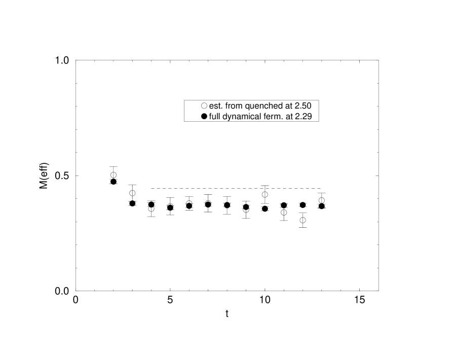
FIG. 1.: Effective meson masses in the Schwinger model calculated with a true action (full dynamical fermion) simulation ($\beta=2.29,\kappa=0.26$) and with a quenched approximate action simulation at $\beta=2.50$.

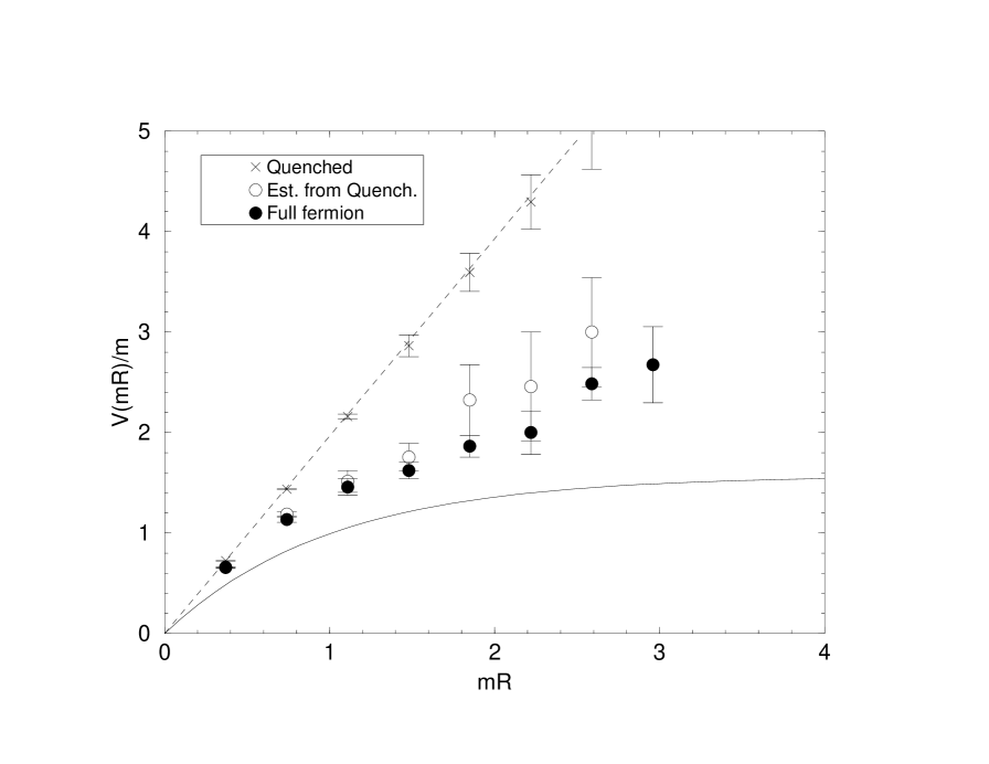
FIG. 2.: The static potential in physical units calculated in three different ways. Crosses indicate the quenched, $\beta=2.50$ result, open circles indicate the deficit corrected quenched results and the filled circles are the full dynamical fermion results for $\beta=2.29,\kappa=0.25$. The curves are described in the text.

FIG. 3.: Loops included in the first attempt to improve on the quenched approximation for the Schwinger model.

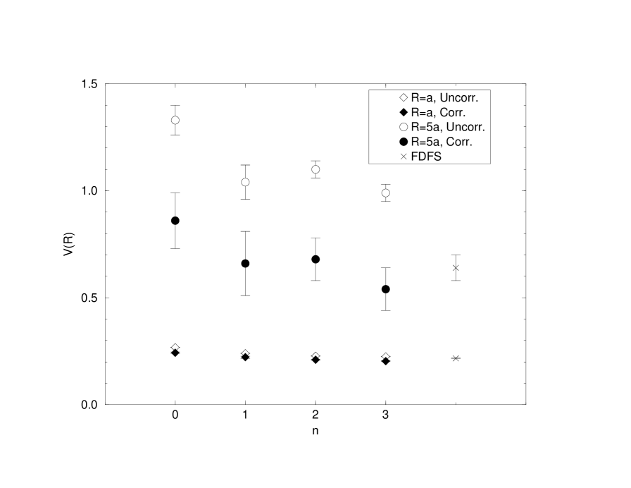
FIG. 4.: The static potential in lattice units using different orders of approximation. Open symbols denote raw measurements at a given order, while full symbols denote deficit corrected results. The corresponding full dynamical simulation results are indicated by the crosses at the right of the diagram.

FIG. 5.: Loops which give the optimum approximation to the true Schwinger model dynamical fermion action.

REFERENCES

- [1] J. C. Sexton and D. H. Weingarten, Nucl. Phys. B (Proc. Suppl.) 42 (1995) 361; J. C. Sexton and D. H. Weingarten, preprint heplat/9411029.
- [2] A. C. Irving and J. C. Sexton, Nucl. Phys. B (Proc. Suppl.) 47 (1996) 679
- [3] G. Kilcup, Phys. Rev. D. (to appear).
- [4] C. Bernard and M. Golterman, Nucl. Phys. B (Proc. Suppl.) 30 (1993) 217; C. Bernard et al, Nucl. Phys. B (Proc. Suppl.) 47 (1996) 345.
- [5] M. Lüscher, Nucl. Phys. B 418 (1994) 637.
- [6] G. M. de Divitiis, R. Frezzotti, M. Guagnelli, M. Masetti and R. Petronzio, Nucl. Phys. B 455 (1995) 274; G. M. de Divitiis et al., Rome preprint ROM2F-96-16, heplat/9605002
- [7] S. Duane, A. D. Kennedy, B. J. Pendleton and D. Roweth, Phys. Lett. B 195 (1987) 2.
- [8] J. C. Sexton and D. H. Weingarten, Nucl. Phys. B 380 (1992) 665.
- [9] G. H. Golub and C. F. Van Loan, Matrix Computions, John Hopkins University Press, 1983.
- [10] M. B. Halpern, Phys. Rev. D 13 (1976) 337.
- [11] H. van der Vorst, SIAM J. Sc. Stat. Comp. 13 (1992) 631.
- [12] M. Peardon, Nucl. Phys. B (Proc. Suppl.) 42 (1995) 891
- [13] A. Boriçi and Ph. de Forcrand, Nucl. Phys. B 418 (1994) 637; A. Borrelli, Ph. de Forcrand and A. Galli, Max Plank preprint, hep-lat/9602016