Continuum Limit of the Heavy-Light Decay Constant with the Quenched Wilson Quark Action

Abstract

We explore the problems in calculating the decay constant for heavy-light mesons using the quenched Wilson quark action for both heavy and light quarks. We find that the continuum limit of the decay constant is reasonably converged among different prescriptions after the continuum limit is taken. A number of technical problems associated with prescriptions are also addressed.

1 Introduction

Extrapolation to the continuum limit is an indispensable procedure to obtain physics from lattice calculations. For the system including heavy quarks ($Q$) this extrapolation might no longer be straightforward, since $O(m_{Q}a)$ errors can uncontrollably be large. In this work we numerically explore the problem of the continuum limit for the decay constant of heavy-light mesons using the Wilson heavy quark action in the quenched approximation.

2 Simulation

Table 1 summarizes parameters we used in our simulations carried out on VPP-500/80 at KEK. The improvement we have made since Lattice 95[1] is the adoption of a smeared source for heavy quarks to suppress contaminations from excited states, and an addition of a run at $\beta=5.9$. We use as a smearing function the wave function of heavy-light mesons as measured in the simulation. The size of lattice is chosen so that physical volume is roughly constant against $\beta$. We take the physical scale of the lattice estimated from the charmonium spin-averaged 1S-1P mass splitting.

Table 1: Simulation Parameters

$\beta$	5.9	6.1	6.3
size	$\mbox{16}^{3}\times\mbox{40}$	$\mbox{24}^{3}\times\mbox{64}$	$\mbox{32}^{3}\times\mbox{80}$
#conf.	150	100	100
$a_{1S-1P}^{-1}$(GeV)	1.84(03)	2.54(07)	3.36(11)

3 Kinetic versus pole mass

The effective Hamiltonian for Wilson quark with a large mass $m_{Q}a$ takes the form[2],

$$H=\bar{\Psi}\left[m_{pole}-\frac{\mbox{\boldmath D}^{2}}{2m_{kin}}-\frac{\mbox{\boldmath$\sigma$}\cdot\mbox{\boldmath B}}{2m_{mag}}+\cdots\right]\Psi,$$ (1)

where all mass parameters may differ by $O(m_{Q}a)$.

In Figure 1 we plot $m_{kin}a-m_{pole}a$ as a function of the bare quark mass for heavy-light and heavy-heavy mesons, where $m_{kin}a$ is extracted from measured dispersion relations. We expect the two results to agree, since the binding energy should cancel in the mass difference. The data, however, show that they do not, implying that we cannot determine the kinetic mass consistently from heavy-light and heavy-heavy systems[3]. Even worse, as $\beta$ increases, $m_{kin}a-m_{pole}a$ undershoots and becomes negative in a region $m_{Q}a\hbox to0.0pt{\lower 3.5pt\hbox{$\mathchar 0\relax\sim$}\hss}\raise 1.0pt\hbox{$<$}0.7$.

Figure 1: $m_{kin}a-m_{pole}a$ for heavy-light (filled symbols) and $(m_{kin}a-m_{pole}a)/2$ for heavy-heavy (open symbols) mesons. Dashed curve represents tree level value for free Wilson quark.

We plot in Figure 2 $2m_{Q\bar{q}}-m_{Q\bar{Q}}$, with $m_{Q\bar{q}}$ mass of a heavy-light meson and $m_{Q\bar{Q}}$ for a heavy-heavy meson. This mass difference as obtained with the two mass definitions is compared with experimental values (asterisks). The pole mass gives values close to the experiment, while the results with the kinetic mass definition stays far away from the experiment. Whereas we naively expect that $m_{kin}$ is the most adequate mass parameter of the system, as the kinetic energy term dominantly controls the dynamics of the system, our results show that the kinetic mass measured from simulations suffers from the effects arising from higher order terms of $1/m_{Q}$ which receive large finite lattice corrections[4]. For this reason we cannot conclude that the use of the kinetic mass is superior to the pole mass.

Figure 2: $2m_{Q\bar{q}}-m_{Q\bar{Q}}$ calculated with pole mass (filled symbols) and kinetic mass (open symbols) as compared with experiment(asterisks).

4 Heavy-Light Decay Constant

We study the problem of the continuum limit by taking a number of alternative prescriptions for the meson mass parameter and the wave function normalization. (IA) The simplest choice is use of the pole mass and the naive normalization $(2K_{Q})^{1/2}$. (IB) Alternatively, we may take $(8K_{c}-6K_{Q})^{1/2}=(2K_{Q})^{1/2}e^{m_{pole}^{(quark)}a/2}$ as the wave function normalization (referred to as the KLM normalization). (IIA) The next choice is use of the kinetic mass obtained from simulations together with the KLM normalization. In this prescription $O(m_{Q}a)$ corrections are removed from leading terms of $1/m_{Q}$. (IIB) In order to avoid the pathology we have seen with the kinetic mass, we may consider yet another definition of the ‘kinetic mass’ estimated from the pole mass using the tree level relation[5], $m_{kin}^{(meson)}=m_{pole}^{(meson)}+(m_{kin}^{(quark)}-m_{pole}^{(quark)})$, while keeping the KLM normalization. The tadpole improved perturbative $Z$-factor is used throughout our analysis.

Figure 3 shows the scale invariant quantity $\Phi_{P}(m_{P})=[\alpha_{s}(m_{P})/\alpha_{s}(m_{B})]^{2/\beta_{0}}f_{P}\sqrt{m_{P}}$ as a function of $1/m_{P}$ for cases (IA) and (IIB). The naive normalization gives significantly smaller values than the KLM normalization does for heavy quarks; as is well known $f_{P}\sqrt{m_{P}}$ even decreases towards a large quark mass. This contrasts to case (IIB), in which it increases with the meson mass and is smoothly extrapolated to the value estimated in the static limit[6]. The method (IB) also approaches the static limit, the difference from (IIB) being an $O(e^{-m_{P}})$ finite mass correction rather than $O(1/m_{P})$[5].

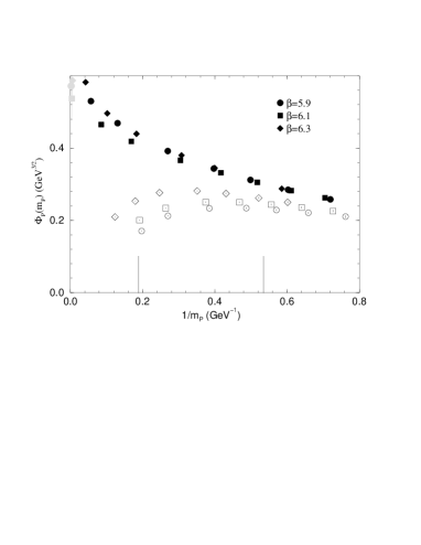
Figure 3: $\Phi_{P}(m_{P})$ versus $1/m_{P}$ with the prescription IA (open symbols) and with IIB (filled symbols). Results with the static approximation are also shown at $1/m_{P}$=0.

Extrapolation to the continuum limit is illustrated in Figure 4 for $f_{D_{s}}$ assuming linear $O(m_{Q}a)$ behavior. Roughly speaking, all prescriptions give a reasonably convergent answer, and the variation from one to another is an $O((m_{Q}a)^{2})$ effect. At a more precise look, however, the result for (IIA) is sizably deviated from the others. This is apparently caused by a pathological behavior of $m_{kin}a-m_{pole}a$ in the charm mass region as discussed above. We note that the simplest prescription (IA) gives a result in agreement with the others in spite of a large extrapolation. The difference from (IB) by an exponential factor $e^{m_{pole}^{(quark)}a/2}$ in the KLM normalization does not invalidate the linear extrapolation for this case since $O((m_{Q}a)^{2})$ terms are small for c-quark.

The results for $f_{B_{s}}$ are also well convergent in the continuum limit (Figure 5). Although the remaining systematic uncertainty cannot be properly estimated for the prescription using the pole mass for $m_{Q}a$ is larger than unity for the $b$-quark, we expect that the remaining errors are reasonably small for (IIB).

After continuum extrapolation we obtain $f_{D}$ = 202(8)${}^{+24}_{-11}$ MeV $f_{D_{s}}$ = 216(6)${}^{+22}_{-15}$ MeV $f_{B}$ = 179(11)${}^{+2}_{-31}$ MeV $f_{B_{s}}$ = 197(7)${}^{+0}_{-35}$ MeV where we take the value with prescription (IIB) for our central values. The first error is statistical and the second represents a spread over four prescriptions, which gives an estimate of $O((m_{Q}a)^{2})$. Finally we emphasize that convergence of different extrapolations to the continuum limit both from above and below bolsters the reliability of our results, at least for charmed mesons. We expect that the errors for bottom mesons are at most within the quoted errors.

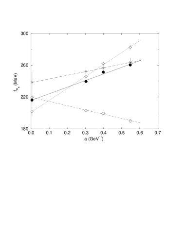
Figure 4: Continuum extrapolation of $f_{D_{s}}$ with four methods: IA (open circles), IB (open diamonds), IIA (crosses) and IIB (filled circles)

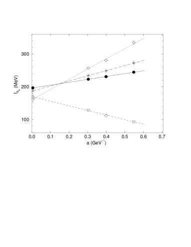
Figure 5: Same as Figure 4 for $f_{B_{s}}$.

References

- [1] S. Aoki et al. (JLQCD Collaboration), Nucl. Phys. B (Proc. Supple.) 47 (1996) 433.
- [2] A.X. El-Khadra, A.S. Kronfeld and P.B. Mackenzie, hep-lat/9604004.
- [3] S. Collins et al., Nucl. Phys. B (Proc. Supple.) 47 (1996) 455.
- [4] A.S. Kronfeld, these proceedings.
- [5] C.W. Bernard, J.N. Labrenz and A. Soni, Phys. Rev. D49 (1994) 2536.
- [6] A. Duncan et al., Phys. Rev. D51 (1995) 5101.