Critical exponents and abelian dominance in $SU(2)$ QCD

Abstract

The critical properties of the abelian Polyakov loop and the Polyakov loop in terms of Dirac string are studied in finite temperature abelian projected $SU(2)$ QCD. We evaluate the critical point and the critical exponents from each Polyakov loop in the maximally abelian gauge using the finite-size scaling analysis. Abelian dominance in this case is proved quantitatively. The critical point of each abelian Polyakov loop is equal to that of the non-abelian Polyakov loop within the statistical errors. Also, the critical exponents are in good agreement with those from non-abelian Polyakov loops.

I Introduction

Abelian projected QCD has been studied extensively in recent years, for elucidating the mechanism of quark confinement [1, 2]. The abelian projection of QCD[3] is to perform a partial gauge-fixing such that the maximal abelian torus group remains unbroken. Abelian monopoles appear as a topological quantity in such a partial gauge fixing, so that QCD can be regarded as an abelian theory with electric charges and monopoles. ’t Hooft conjectured that if the monopoles made Bose condensation, quarks could be confined due to dual Meissner effect[3].

There are some evidences on lattices that the abelian theory in the maximally abelian (MA) gauge[4] well represents the long range properties of QCD:

1. Abelian Wilson loops composed of abelian link fields alone can reproduce the full ($SU(2)$) value of the string tension. Furthermore, the abelian Wilson loops written in terms of monopole currents also reproduce the value [5, 6, 7, 8, 9, 10].

2. Polyakov loops written in terms of abelian fields and also in terms of Dirac strings of monopoles (monopole Polyakov loops) can reproduce the behavior of non-abelian Polyakov loops [11].

3. A monopole effective action can be calculated. The argument of the energy and the entropy indicates that QCD is in the monopole condensed phase[7, 12].

These facts are usually called abelian (monopole) dominance in quark confinement and suggest that ’t Hooft’s conjecture[3] is realized in MA gauge.

Figure 1 shows the non-abelian, the abelian and the monopole Polyakov loops versus $\beta$ on $24^{3}\times 4$ $SU(2)$ lattice[11]. The abelian and the monopole Polyakov loops change drastically around the critical point $\beta$=2.29 determined from the non-abelian Polyakov loops. The abelian and the monopole Polyakov loops appear to be good order parameters. However, those curves seem to have different slopes. Their absolute values in the deconfinement phase are also different. Actually, those three, the non-abelian, the abelian and the monopole Polyakov loops are quite different operators.

The critical property of 4-dimensional $SU(2)$ lattice gauge theory is shown to be universal to that of 3-dimensional $Z_{2}$ theory [13]. It is interesting to study what exponents are calculated from the abelian and the monopole Polyakov loops at each critical point, since $Z_{2}$ symmetry is not so directly understood in the framwork of monopole dynamics[14] and there is no reason the exponents of those different Polyakov loops agree with each other. Such a study helps us also to test how good the abelian dominance is quantitatively. It is the aim of this work.

II Definition of abelian and monopole Polyakov loops

A non-abelian Polyakov loop in $SU(2)$ lattice gauge theory is written in the form

$$P_{SU(2)}(x_{0})=\frac{1}{2}\mbox{Tr}\prod_{t}U_{4}(x_{0},t),$$ (1)

where $U_{\mu}(x,t)$ are $SU(2)$ link variables at space $x$ and at time $t$.

After abelian projection is over, we can define abelian Polyakov loops[6] written in terms of abelian link variables. The abelian link variables can be separated from gauge-fixed link variables

$$\widetilde{U}_{\mu}(x,t)=C_{\mu}(x,t)u_{\mu}(x,t),$$ (2)

where $\widetilde{U}_{\mu}(x,t)$ is a gauge-fixed link variable. $u_{\mu}(x,t)$ is a diagonal matrix composed of phase factors of the diagonal components of $\widetilde{U}_{\mu}(x,t)$. We can define an abelian Polyakov loop

$$P_{abel}(x_{0})=\mbox{Re\,}[\exp(i\sum_{x,t}\theta_{4}(x,t)J_{4}(x,t))].$$ (3)

Here $J_{\mu}(x,t)=\delta_{\mu,4}\delta_{x,x_{0}}$ and $\theta_{\mu}(x,t)$ are the angle variables of $u_{\mu}(x,t)$:

$$u_{\mu}(x,t)=\left(\begin{array}[]{cc}\exp(i\theta_{\mu}(x,t))&0\\ 0&\exp(-i\theta_{\mu}(x,t))\end{array}\right).$$ (6)

The abelian Polyakov loop can be decomposed into two parts: a monopole part and a photon part[11]. An abelian field strength can be written as

$$f_{\mu\nu}(x,t)=\partial_{\mu}\theta_{\nu}(x,t)-\partial_{\nu}\theta_{\mu}(x,t),$$ (7)

where $\partial_{\nu}$ is a forward derivative. Rewriting this equation, we get

$$\theta_{\mu}(x,t) = -\sum_{x^{\prime},t^{\prime}}D(x-x^{\prime},t-t^{\prime})\partial^{\prime}_{\nu}f_{\nu\mu}(x^{\prime},t^{\prime})-\sum_{x^{\prime},t^{\prime}}D(x-x^{\prime},t-t^{\prime})\partial_{\mu}\partial^{\prime}_{\nu}\theta_{\nu}(x^{\prime},t^{\prime}),$$ (8)

where $\partial^{\prime}_{\nu}$ is a backward derivative and $D(x,t)$ is a lattice Coulomb propagator which satisfies $\partial^{\prime}_{\mu}\partial_{\mu}D(x,t)=-\delta_{x,0}\delta_{t,0}$. Then the abelian Polyakov loop (Eq.(3)) can be written in terms of the abelian field strength:

$$P_{abel}(x_{0})=\mbox{Re\,}[\exp(-i\sum_{x,t,x^{\prime},t^{\prime}}D(x-x^{\prime},t-t^{\prime})\partial^{\prime}_{\nu}f_{\nu 4}(x^{\prime},t^{\prime})J_{4}(x,t))].$$ (9)

Here the second term of Eq.(8) vanishes owing to $\partial_{4}J_{4}(x,t)=0$. The abelian field strength can be separated into two parts:

$$f_{\nu\mu}=\bar{f}_{\nu\mu}+2\pi n_{\nu\mu},$$ (10)

where $n_{\nu\mu}$ is an integer and $\bar{f}_{\nu\mu}\in[-\pi,\pi)$. Then, rewriting Eq.(9), we get

$$P_{abel}(x_{0}) = \mbox{Re\,}[\exp(-i\sum_{x,t,x^{\prime},t^{\prime}}D(x-x^{\prime},t-t^{\prime})\partial^{\prime}_{\nu}\bar{f}_{\nu 4}(x^{\prime},t^{\prime})J_{4}(x,t))$$ (12)

$$\;\times\exp(-2\pi i\sum_{x,t,x^{\prime},t^{\prime}}D(x-x^{\prime},t-t^{\prime})\partial^{\prime}_{\nu}n_{\nu 4}(x^{\prime},t^{\prime})J_{4}(x,t))]$$

$$= \mbox{Re\,}[P_{1}(x_{0})\cdot P_{2}(x_{0})].$$ (13)

The monopole Polyakov loop, $P_{mono}(x_{0})=\mbox{Re\,}P_{1}(x_{0})$ is composed of Dirac strings of monopoles. $P_{photon}(x_{0})=\mbox{Re\,}P_{2}(x_{0})$ only contains the contributions from photons. Suzuki et al.[11] have indicated that

1. $P_{abel}(x_{0})\sim P_{mono}(x_{0})\times P_{photon}(x_{0})$ in MA gauge.

2. $P_{abel}(x_{0})$, $P_{mono}(x_{0})$ and $P_{SU(2)}(x_{0})$ vanish for $\beta<\beta_{c}$.

3. $P_{photon}$ is finite from $\beta=$2.1 to 2.5 and does not change drastically around the critical point.

III Finite-size scaling theory

We calculated the critical exponent of the non-abelian, the abelian and the monopole Polyakov loops from a finite-size scaling theory. The singular part of the free energy density on $N_{s}^{3}\times N_{t}$ lattice has the following form:

$$f_{s}(x,h,N_{s})=N_{s}^{-d}Q_{s}(xN_{s}^{1/\nu},hN_{s}^{(\beta+\gamma)/\nu},g_{i}N_{s}^{y_{i}}),$$ (14)

where $x=(T-T_{c})/T_{c}$. Here the action contains the term $hN_{s}^{d}L$ ($L$ denotes the magnetization) and $g_{i}$ are the irrelevant fields with exponent $y_{i}$. By differentiating $f_{s}$ with respect to $h$ at $h=0$, we get

$$\langle L\rangle(x,N_{s}) = N_{s}^{-\beta/\nu}Q_{L}(xN_{s}^{1/\nu},g_{i}N_{s}^{y_{i}}),$$ (15)

$$\chi(x,N_{s}) = N_{s}^{\gamma/\nu}Q_{\chi}(xN_{s}^{1/\nu},g_{i}N_{s}^{y_{i}}),$$ (16)

$$g_{r}(x,N_{s}) = Q_{g_{r}}(xN_{s}^{1/\nu},g_{i}N_{s}^{y_{i}}),$$ (17)

where $\langle L\rangle$, $\chi$ and $g_{r}$ are order parameter, susceptibility and 4-th cumulant, respectively:

$$L = \frac{1}{N_{s}^{3}}\sum_{x}P(x),$$ (18)

$$\chi = N_{s}^{3}(\langle L^{2}\rangle-\langle L\rangle^{2}),$$ (19)

$$g_{r} = \frac{\langle L^{4}\rangle}{{\langle L^{2}\rangle}^{2}}-3.$$ (20)

Expanding these equations with respect to $x$, we have at $x=0$

$$\langle L\rangle(x=0,N_{s}) = N_{s}^{-\beta/\nu}(c_{0}+c_{3}N_{s}^{-\omega}),$$ (21)

$$\chi(x=0,N_{s}) = N_{s}^{\gamma/\nu}(c_{0}+c_{3}N_{s}^{-\omega}),$$ (22)

$$g_{r}(x=0,N_{s}) = c_{0}+c_{3}N_{s}^{-\omega},$$ (23)

where we take only the largest irrelevant exponents ($-\omega$) into account. We can calculate the critical point from the fit to the $N_{s}$-behavior of those equations. The critical point can be defined as the point where a fit to the leading $N_{s}$-behavior has the least $\chi^{2}$[15]. Actually, the leading $N_{s}$-behavior of Eq.(21) and of Eq.(22) is given by

$$\ln\langle L\rangle(x=0,N_{s}) = -\frac{\beta}{\nu}\ln N_{s}+\ln c_{0},$$ (24)

$$\ln\chi(x=0,N_{s}) = \frac{\gamma}{\nu}\ln N_{s}+\ln c_{0}.$$ (25)

From the fits to Eqs.(23), (24) and (25), we can find the position of the critical point $\beta_{c}$, and obtain the values of $\beta/\nu$, $\gamma/\nu$ and $g_{r}^{\infty}$ at $\beta_{c}$ simultaneously. Here $g_{r}^{\infty}$ is the value of $g_{r}$ on the infinite volume and is denoted by $c_{0}$ in Eq.(23). We also considered the derivatives of the observables with respect to $x$. The $N_{s}$-behavior of each derivative is given by

$$\frac{\partial\langle L\rangle}{\partial x}(x,N_{s}) = N_{s}^{(1-\beta)/\nu}Q^{\prime}_{L}(xN_{s}^{1/\nu}),$$ (26)

$$\frac{\partial\chi}{\partial x}(x,N_{s}) = N_{s}^{(1+\gamma)/\nu}Q^{\prime}_{\chi}(xN_{s}^{1/\nu}),$$ (27)

$$\frac{\partial g_{r}}{\partial x}(x,N_{s}) = N_{s}^{1/\nu}Q^{\prime}_{g_{r}}(xN_{s}^{1/\nu}).$$ (28)

The leading $N_{s}$-behavior of each equation at the critical point is

$$\ln\frac{\partial\langle L\rangle}{\partial x}(x=0,N_{s}) = \frac{1-\beta}{\nu}\ln N_{s}+\ln d_{0},$$ (29)

$$\ln\frac{\partial\chi}{\partial x}(x=0,N_{s}) = \frac{1+\gamma}{\nu}\ln N_{s}+\ln d_{0},$$ (30)

$$\ln\frac{\partial g_{r}}{\partial x}(x=0,N_{s}) = \frac{1}{\nu}\ln N_{s}+\ln d_{0}.$$ (31)

Hence, $(1-\beta)/\nu$,$(1+\gamma)/\nu$ and $1/\nu$ can also be evaluated from the fits to those equations.

IV Results and Discussions

We performed numerical calculations on $N_{s}^{3}\times 4$ lattices, where $N_{s}=$8, 12, 16 and 24. The standard $SU(2)$ Wilson action was adopted and abelian link valuables were defined in MA gauge. We calculated the observables

$$L = \frac{1}{N_{s}^{3}}\sum_{x}P(x),$$ (32)

where $P(x)$ denotes $P_{SU(2)}(x)$, $P_{abel}(x)$ and $P_{mono}(x)$. Actually, $\chi_{v}=N_{s}^{3}\langle L^{2}\rangle$ was calculated instead of $\chi$, because $\chi_{v}$ is equal to $\chi$ below the critical point [15]. The values of the observables at various $\beta$ are needed in order to calculate the derivatives with respect to $x$, where $x=(\beta-\beta_{c})/\beta_{c}$. We used the density of state method(DSM)[16, 17]. First we performed Monte-Carlo simulations at $\beta=\beta_{0}$, and then calculated the following averages:

$$O(s)=\sum_{k=1}^{N(s)}{O_{k}}/{N(s)},$$ (33)

where $s$ is the value of the action, $N(s)$ the number of the configurations whose action has the same value of $s$, and $O_{k}$ the observable obtained from the $k$-th configuration. The expectation value of the observables in the vicinity of $\beta_{0}$ is then given by

$$\langle O\rangle_{\beta}=\frac{\sum_{s}N(s)O(s)\exp(-\beta s+\beta_{0}s)}{\sum_{s}N(s)\exp(-\beta s+\beta_{0}s)},$$ (34)

where $\beta_{0}=$2.2988 was adopted and $\beta\in$$[2.2980,2.3000]$. $\langle L\rangle$, $\chi$ and $g_{r}$ at $\beta_{0}$ were calculated every 50 sweeps after 2000 thermalization sweeps. The number of samples was 100000, except on $24^{3}\times 4$ lattice (47000 in the case). The errors were determined according to the Jackknife method dividing the entire sample into 10 blocks (4 blocks on $24^{3}\times 4$ lattice).

We estimated the critical point $\beta_{c}$ from the $\chi^{2}$ method. The data of our DSM results were fitted to Eqs.(23)-(25) and Eqs.(29)-(31) at each $\beta$. The number of input data was 2 and that of fit parameters was 2 ($\omega$ in Eq.(23) was fixed to 1 in accordance with Engels et al.[15]). Figure 2 describes the typical curves of $\chi^{2}/N_{f}$ versus $\beta$. Here the number of degrees of freedom, $N_{f}$ is 2. Each curve in Fig. 2 is smooth and has its minimum value. Table I shows the positions of minimal $\chi^{2}/N_{f}$ for all observables obtained. Almost all the $\chi^{2}_{min}/N_{f}$ are small. However, the $\chi^{2}_{min}/N_{f}$ were not seen from our $\partial g_{r}/\partial x$ fits. Furthermore, our two-parameter fits were not so good in the cases of $\langle L\rangle$, $\chi$, $\partial\langle L\rangle/\partial x$ and $\partial\chi/\partial x$ from the monopole Polyakov loops. Then we used Eq.(21) and Eq.(22) for their fits which contained three parameters to be fitted. The values of $\omega$ in Eq.(21) and Eq.(22) were chosen in such a way that the values of $\chi^{2}_{min}/N_{f}$ became as small as possible.

Averaging the obtained minimal positions of $\chi^{2}_{min}/N_{f}$, we get

$$\beta_{c}^{SU(2)} = 2.29940(20),$$ (35)

$$\beta_{c}^{abel}\;\;\, = 2.99962(26),$$ (36)

$$\beta_{c}^{mono}\; = 2.29971(23).$$ (37)

The critical points obtained from the abelian and the monopole Polyakov loop are very close to the non-abelian critical point as expected from Fig. 1.

Table II lists the critical exponents on each critical point in the non-abelian, the abelian and the monopole case. The non-abelian exponents obtained by Engels et al.[15], the exponents of 3-dimensional Ising model[13] and those of $U(1)$[18] are also shown. The errors were caused by fluctuations of the interpolated DSM data and by uncertainty of each $\beta_{c}$. See also Fig. 3. Those critical exponents seem to be reliable because of the following reasons: three $\nu$’s obtained from three different fits are within the statistical errors; hyperscaling relations are well satisfied; non-abelian exponents obtained are consistent with those of Engels et al.[15]. Table II shows the following notable results:

1. The critical exponents in the abelian and the monopole case are in agreement with non-abelian exponents within the statistical error.

2. Those critical exponents agree with those of $Z_{2}$ rather than those of $U(1)$.

The abelian (monopole) dominance in quark confinement is proved quantitatively in this case.

There remain some problems to be studied further. The critical points obtained are outside the one-sigma error bar of Engels et al.[15]; minimal $\chi^{2}/N_{f}$ were not seen for some fits; some values of $\chi^{2}_{min}/N_{f}$ are $O(1)$ which are not small enough. These problems seem to reflect a lack of statistics. More samples may be needed especially on $24^{3}\times 4$ lattice.

The simulations of this work were carried out on VPP500 at Institute of Physical and Chemical Research (RIKEN) and at National Laboratory for High Energy Physics at Tsukuba (KEK). This work is financially supported by JSPS Grant-in Aid for Scientific Research (B) (No.06452028).

		$\beta|_{\chi^{2}_{min}}$	$\chi^{2}_{min}/N_{f}$			$\beta|_{\chi^{2}_{min}}$	$\chi^{2}_{min}/N_{f}$
$g_{r}$	SU(2)	2.29952	1.49	${\partial g_{r}}/{\partial x}$	SU(2)	$-$	$<O(10^{-1})$
	abel	2.29936	1.27		abel	$-$	$<O(10^{-1})$
	mono	2.29974	0.47		mono	$-$	$<O(10^{-1})$
$\langle L\rangle$	SU(2)	2.29960	1.33	${\partial\langle L\rangle}/{\partial x}$	SU(2)	2.29920	0.004
	abel	2.29984	0.95		abel	2.29938	0.017
	mono	$-$	$<O(1)$		mono	2.29948	$6\times 10^{-7}$
$\chi$	SU(2)	2.29946	1.33	${\partial\chi}/{\partial x}$	SU(2)	2.29924	0.005
	abel	2.29986	0.75		abel	2.29964	0.061
	mono	$-$	$<O(1)$		mono	2.29992	$6\times 10^{-6}$

TABLE I.: The positions of minimal $\chi^{2}/N_{f}$ and the value of $\chi^{2}_{min}/N_{f}$ in the non-abelian,the abelian and the monopole cases.

	$SU(2)$	abel	mono	Engels et al.[15]	Ising[13]	$U(1)$[18]
$\beta/\nu$	0.504(18)	0.485(22)	0.528(64)	0.525(8)	0.518(7)
$(1-\beta)/\nu$	1.117(27)	1.138(10)	1.091(84)	1.085(14)	1.072(7)
$\nu$	0.617(16)	0.616(12)	0.617(57)	0.621(6)	0.6289(8)	0.67
$\beta$	0.311(19)	0.299(19)	0.326(69)	0.326(8)	0.3258(44)	0.35
$\gamma/\nu$	1.977(29)	2.025(34)	1.991(88)	1.944(13)	1.970(11)
$(1+\gamma)/\nu$	3.600(38)	3.646(44)	3.608(93)	3.555(15)	3.560(11)
$\nu$	0.616(25)	0.617(29)	0.618(68)	0.621(8)	0.6289(8)
$\gamma$	1.218(68)	1.249(81)	1.23(19)	1.207(24)	1.239(7)	1.32
$\gamma/\nu+2\beta/\nu$	2.985(47)	2.995(56)	3.05(15)	2.994(21)	3.006(18)
$-g_{r}^{\infty}$	1.447(41)	1.438(42)	1.438(41)	1.403(16)	1.41
$\nu$	0.633(13)	0.621(14)	0.600(13)	0.630(11)	0.6289(8)

TABLE II.: The critical exponents calculated from the non-abelian, the abelian and the monopole Polyakov loops at each critical point.

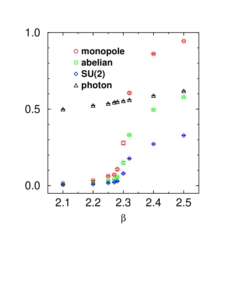
FIG. 1.: Non-abelian, abelian and monopole Polyakov loops in $SU(2)$ QCD on $24^{3}\times 4$ lattices.

FIG. 2.: $\chi^{2}/N_{f}$ from $g_{r}$ fits and from $\partial\langle L\rangle/\partial x$ fits versus $\beta$ in the non-abelian, the abelian and the monopole cases. The number of degrees of freedom, $N_{f}$ is 2.

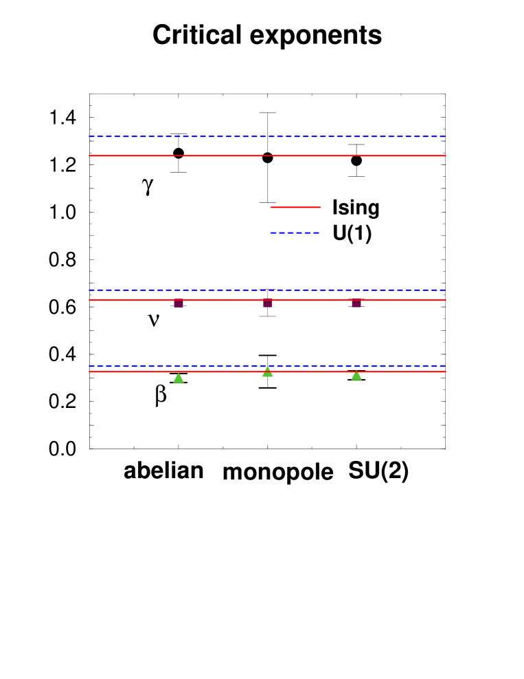
FIG. 3.: Critical exponents of non-abelian, abelian and monopole Polyakov loops in $SU(2)$ QCD.

REFERENCES

• [1] T. Suzuki, Nucl. Phys. B(Proc. Suppl.) 30 (1993) 176 and references therein.
• [2] M. Polikarpov, Talk at Lattice 96, to appear in Nucl. Phys. B(Proc. Suppl.).
• [3] G. ’tHooft, Nucl. Phys. B190 (1981) 455.
• [4] A.S. Kronfeld $et$ $al.$, Phys. Lett. B198 (1987) 516;
A.S. Kronfeld, G. Schierholz and U.-J. Weise, Nucl.Phys. B293 (1987) 461.
• [5] T. Suzuki and I. Yotsuyanagi, Phys. Rev. D42 (1990) 4257; Nucl. Phys. B(Proc. Suppl.) 20 (1991) 236.
• [6] S. Hioki $et$ $al.$, Phys. Lett. B272 (1991) 326.
• [7] H. Shiba and T. Suzuki, Nucl. Phys. B(Proc. Suppl.) 34 (1994) 182 .
• [8] H. Shiba and T. Suzuki, Phys. Lett. B333 (1994) 461.
• [9] S. Ejiri, S. Kitahara, Y. Matsubara and T. Suzuki, Phys. Lett. B343 (1995) 304.
• [10] J.D. Stack, R.J. Wensley and S.D. Neiman, Phys.Rev. D50 (1994) 3399.
• [11] T. Suzuki $et$ $al.$, Phys. Lett. B347 (1995) 375.
• [12] H. Shiba and T. Suzuki, Phys. Lett. B351 (1995) 519.
• [13] A.M. Ferrenberg and D.P. Landau, Phys. Rev. B44 (1991) 5081.
• [14] S. Ejiri, Talk at Lattice 96, to appear in Nucl. Phys. B(Proc. Suppl.).
• [15] J. Engels $et$ $al.$, University of Bielefeld preprint, BI-TP 95/29, 1995.
• [16] A.M. Ferrenberg and R.H. Swendsen, Phys. Rev. Lett. 63 (1989) 1195.
• [17] J. Engels, J. Fingberg and D. E. Miller, Nucl. Phys. B387 (1992) 501.
• [18] B. Svetitsky Phys. Pep. 132 (1986) 1.