Monopole action and monopole condensation
in SU(3) lattice QCD

Abstract

Effective monopole actions for various extended monopoles are derived from vacuum configurations after abelian projection in the maximally abelian gauge in $T=0$ and $T\neq 0$ $SU(3)$ lattice QCD. The actions obtained appear to be independent of the lattice volume adopted. At zero temperature, monopole condensation is seen to occur from energy-entropy balance in the strong coupling region. Larger $\beta$ is included in the monopole condensed phase as more extended monopoles are considered. The scaling seen in the $SU(2)$ case is not yet observed. The renormalization flow diagram suggests the existence of an infrared fixed point. A hysteresis behavior is seen around the critical temperature in the case of the $T\neq 0$ action.

I Introduction

The dual Meissner effect is believed to be the promising candidate for the quark confinement mechanism [1, 2]. This picture is realized in the confinement phase of lattice compact QED[3, 4, 5]. In QCD, the ’tHooft idea [6] of abelian projection is very interesting. The abelian projection is to extract an abelian gauge theory by performing a partial gauge-fixing. Abelian projected QCD can be regarded as an abelian theory with electric charges and magnetic monopoles. ’tHooft conjectured that the condensation of the abelian monopoles causes the confinement in QCD.

Many works have been done to test the idea in the framework of lattice QCD using Monte-Carlo simulations. An interesting abelian projection called maximally abelian (MA) gauge [7] is found. $U(1)^{2}$ invariant operators written in terms of abelian link fields alone after the abelian projection reproduce essential features of confinement phenomena like the string tension [8], the Polyakov loop, thermodynamic quantities [9, 10] and even chiral condensate and hadron masses [11, 12, 13, 14]. This is called abelian dominance.

Such $U(1)^{2}$ invariant abelian operators can be decomposed into a product of a monopole operator written in terms of monopole currents or Dirac string and a photon one containing photon contribution alone [15, 16, 17]. The above phenomena called abelian dominance are shown to be reproduced by the monopole contributions alone (monopole dominance) [12, 13, 14, 15, 16, 17, 18].

Such phenomena called abelian and monopole dominance strongly suggest that low-energy QCD can be described by an effective abelian theory. Actually it is possible to derive an effective theory of an extended Wilson form in terms of the abelian link field alone [10]. But the action derived needs larger and larger Wilson loops when we go to higher $\beta$ in the scaling region, although it takes a simple Wilson action like in compact QED in the strong coupling region.

The monopole dominance implies the existence of an effective action on the dual lattice in terms of a dual quantity like monopole currents. In the case of compact QED, the exact dual transformation can be done and leads us to an action describing a monopole Coulomb gas, when one adopt the partition function of the Villain form [4, 19, 20, 21]. Monopole condensation is shown to occur in the confinement phase from energy-entropy balance of monopole loops.

In the case of QCD, however, we encounter a difficulty in performing the exact dual transformation. Shiba and one of the present author (T.S.) have succeeded in numerically carrying out the dual transformation to obtain a monopole action from the vacuum ensemble of monopole currents [22, 23, 24, 25, 26]. This can be done by extending the Swendsen method[27]. They also have performed a block-spin transformation on the dual lattice by considering extended monopoles [28]. The monopole action determined in $SU(2)$ show the following interesting behaviors:

1. A compact and local form of the monopole action is obtained even in the scaling region. The coupling constant of the self-interaction is dominant and the coupling constants decrease rapidly as the distance between the two monopole currents increases.

2. Coupling constants $f_{i}$ for any effective action look volume independent.

3. Monopole condensation is seen to occur for smaller $\beta$ from energy-entropy balance.

4. $f_{i}$ look to show a scaling behavior, that is, they are written only by a physical scale defined by $b=na(\beta)$. This suggests that the $SU(2)$ monopole action is near the renormalized trajectory of the block spin transformation.

5. If the scaling holds good even on the infinite lattice, the $SU(2)$ QCD vacuum is always (for all $\beta$) in the monopole condensed and then confined phase.

To extend this method to $SU(3)$ QCD is very interesting, but it is not so straightforward. There are two independent monopole currents and, to speak more rigorously, three currents $k^{i}_{\mu}(s)$ satisfying one constraint $\sum_{i}k^{i}_{\mu}(s)=0$. There is a permutation symmetry (Weyl symmetry) with respect to the species. Calculating the entropy becomes very difficult as naturally expected. Hence we try to construct an effective action composed of only one monopole current after integrating out the other two. Then the entropy may be evaluated similarly as done in $SU(2)$ and in compact QED. It is the aim of this note to report the results of $SU(3)$ QCD[26, 29].

II MA gauge and monopole currents in $SU(3)$

The MA gauge is given on a lattice by performing a local gauge transformation

$$\widetilde{U}_{\mu}(s)=V(s)U_{\mu}(s)V^{-1}(s+\hat{\mu})$$ (1)

such that a quantity

$$R = \sum_{s,\mu,a}{\rm Tr}\Big{(}U_{\mu}(s)\,\lambda_{a}\,U^{\dagger}_{\mu}(s)\,\lambda_{a}\Big{)},$$ (2)

$$\lambda_{1} = \left(\begin{array}[]{ccc}1&0&0\\ 0&-1&0\\ 0&0&0\end{array}\right),\lambda_{2}=\left(\begin{array}[]{ccc}-1&0&0\\ 0&0&0\\ 0&0&1\end{array}\right),\lambda_{3}=\left(\begin{array}[]{ccc}0&0&0\\ 0&1&0\\ 0&0&-1\end{array}\right)$$ (12)

is maximized. Then a quantity

$$X(s)=\sum_{\mu,a}\,[(U_{\mu}(s)\,\lambda_{a}\,U^{\dagger}_{\mu}(s)+U^{\dagger}_{\mu}(s-\mu)\,\lambda_{a}\,U_{\mu}(s-\mu)),\lambda_{a}]$$ (13)

vanishes. After the gauge fixing is done, an abelian link gauge field $u_{\mu}(s)$ is extracted from $SU(3)$ link variables as follows[30];

$$\tilde{U}_{\mu}(s) \equiv C_{\mu}(s)\,u_{\mu}(s),$$ (14)

$$u_{\mu}(s) = \left(\begin{array}[]{ccc}e^{i\theta_{\mu}^{1}(s)}&0&0\\ 0&e^{i\theta_{\mu}^{2}(s)}&0\\ 0&0&e^{i\theta_{\mu}^{3}(s)}\end{array}\right),\ \ \ \sum_{i=1}^{3}\,\theta_{\mu}^{i}(s)=0\hskip 5.69046pt({\textstyle\rm mod2\pi}),$$ (19)

where

$$\theta_{\mu}^{i}(s) \equiv arg\,([\tilde{U}_{\mu}(s)]_{ii})-\frac{1}{3}\,\phi_{\mu}(s)\hskip 8.53581pt\in(-\frac{4}{3}\pi,\frac{4}{3}\pi),$$ (20)

$$\phi_{\mu}(s) \equiv \left.\sum_{i=1}^{3}\,arg\,([\tilde{U}_{\mu}(s)]_{ii})\,\right|_{\textstyle\rm mod2\pi}\in[-\pi,\pi)$$ (21)

and the plaquette angles $\Theta_{\mu\nu}^{i}(s)$ are given by the sum of link angles $\theta_{\mu}^{i}$ as follows;

$$\Theta_{\mu\nu}^{i}(s) = \partial_{\mu}\theta_{\nu}^{i}-\partial_{\nu}\theta_{\mu}^{i},$$ (22)

$$\sum_{i=1}^{3}\,\Theta_{\mu\nu}^{i} = 2\pi\ell\hskip 8.53581pt(\,\ell\hskip 2.84526pt=\hskip 2.84526pt0,\pm 1).$$ (23)

If $\ell=+1$, the plaquette phases are chosen so that

$$\tilde{\Theta}_{\mu\nu}^{i}(s)=\left\{\begin{array}[]{ll}\Theta_{\mu\nu}^{i}(s)-2\pi&{\rm if}\hskip 8.53581pt\Theta_{\mu\nu}^{i}(s)=\rm{max\,(\Theta_{\mu\nu}^{1},\Theta_{\mu\nu}^{2},\Theta_{\mu\nu}^{3})}\\ \Theta_{\mu\nu}^{i}(s)&{\rm otherwise}\end{array}\right.$$ (26)

If $\ell=-1$,

$$\tilde{\Theta}_{\mu\nu}^{i}(s)=\left\{\begin{array}[]{ll}\Theta_{\mu\nu}^{i}(s)+2\pi&{\rm if}\hskip 8.53581pt\Theta_{\mu\nu}^{i}(s)=\rm{min\,(\Theta_{\mu\nu}^{1},\Theta_{\mu\nu}^{2},\Theta_{\mu\nu}^{3})}\\ \Theta_{\mu\nu}^{i}(s)&{\rm otherwise}.\end{array}\right.$$ (29)

Using $\tilde{\Theta}_{\mu\nu}^{i}(s)$, the monopole current is given by

$$\bar{\Theta}_{\mu\nu}^{i}(s)=\tilde{\Theta}_{\mu\nu}^{i}(s)-2\pi n_{\mu\nu}^{i}(s)\hskip 8.53581pt\in[-\pi,\pi),$$ (30)

$$k_{\mu}^{i}(s)=-\frac{1}{4\pi}\epsilon_{\mu\nu\rho\sigma}\partial_{\nu}\bar{\Theta}_{\rho\sigma}^{i}(s+\hat{\mu}),$$ (31)

$$\sum_{i=1}^{3}\,k_{\mu}^{i}(s)=0.$$ (32)

A block-spin transformation is done by considering $n^{3}$ extended monopoles [28]:

$$k_{\mu}^{(n)i}(s) = -\frac{1}{4\pi}\,\epsilon_{\mu\nu\rho\sigma}\,\partial_{\nu}\bar{\Theta}_{\rho\sigma}^{(n)i}(s+\hat{\mu})$$ (33)

$$= \sum_{i,j,m=0}^{n-1}k_{\mu}^{i}(ns+(n-1)\hat{\mu}+i\hat{\nu}+j\hat{\rho}+m\hat{\sigma})$$ (34)

$$\bar{\Theta}_{\rho\sigma}^{(n)i}(s) \equiv \sum_{i,j=0}^{n-1}\bar{\Theta}_{\rho\sigma}^{i}(ns+i\hat{\rho}+j\hat{\sigma})$$ (35)

III The method

The dual transformation is done as follows:

$$Z = \int e^{-S(U)}\delta(X)\Delta_{F}(U)DU$$ (36)

$$= \int Du[\int Dce^{-S(u,c)}\delta(X)\Delta_{F}(U)]$$ (37)

$$= \int Due^{-S_{eff}(u)}$$ (38)

$$= (\prod\sum)\int Du\delta(k,u)e^{-S_{eff}(u)},$$ (39)

$$= (\prod\sum)e^{-S[k^{i}]},$$ (40)

where $X$ is the quantity (13), $\Delta_{F}(U)$ is the Fadeev-Popov determinant and

$$(\prod\sum) \equiv (\prod_{s,\mu,i}\sum_{k^{i}_{\mu}(s)=-\infty}^{\infty})(\delta_{\partial^{\prime}_{\mu}k^{i}_{\mu}(s),0})\delta(\sum_{j}k^{j}_{\mu}(s)),$$ (41)

$$\delta(k,u) \equiv \delta(k^{i}_{\mu}(s)+\frac{1}{4\pi}\epsilon_{\mu\nu\rho\sigma}\partial_{\nu}\bar{\Theta}_{\rho\sigma}^{i}(s+\hat{\mu})).$$ (42)

The block-spin transformation on the dual lattice [28] is expressed as

$$Z = (\prod\sum)^{\prime}[(\prod\sum)\delta(k_{\mu}^{(n)i}(s)-\sum_{i,j,l=0}^{n-1}k^{i}_{\mu}(ns+(n-1)\hat{\mu}+i\hat{\nu}+j\hat{\rho}+l\hat{\sigma}))e^{-S[k^{i}]}]$$ (43)

$$= (\prod\sum)^{\prime}e^{-S[k^{(n)i}]},$$ (44)

where $(\prod\sum)^{\prime}$ is defined for the extended currents similary as in (41).

As shown above, we try to fix the monopole action after integrating out two monopole currents. The monopole action adopted is composed of various two current interactions $S[k]=\sum_{i}\,f_{i}\,S_{i}[k]$. Practically we have to restrict the number of interaction terms. We adopted 12 types of quadratic interactions in most of these studies as was done in $SU(2)$. The definitions are listed in [22, 25]. Here we show the first important 6 interactions in Fig. 1.

In the $T\neq 0$ QCD, the time extent is finite. Hence, the monopole action is taken as follows:

$$S[k]=\sum_{i}\,(f_{i}^{s}\,S_{i,s}+f_{i}^{t}\,S_{i,t}),$$ (45)

where $S_{i,s}$ are interactions between space-like currents and $S_{i,t}$ are interactions between time-like currents.

We generate thermalized vacuum configurations $U_{\mu}(s)$ and then perform the partial gauge fixing in the MA gauge. Then using the above definition of the monopole and the extended monopoles, we get the vacuum ensemble of $k_{\mu}(s)$ and $k_{\mu}^{(n)}(s)$ currents. The Swendsen method[27] is applied to these current ensembles. Since the dynamical variables $k_{\mu}(s)$ satisfy the conservation rule, it is necessary to extend the original Swendsen method by considering a plaquette $(s^{\prime},\mu^{\prime},\nu^{\prime})$ instead of a link [25, 31]. Introducing a new set of coupling constants $\{\tilde{f}_{i}\}$, define

$$\bar{S}_{i}[k]=\frac{\sum_{M=-\infty}^{\infty}S_{i}[k^{\prime}]\exp(-\sum_{j}\tilde{f}_{j}S_{j}[k^{\prime}])}{\exp(-\sum_{j}\tilde{f}_{j}S_{j}[k^{\prime}])},$$ (46)

where $k^{\prime}_{\mu}(s)=k_{\mu}(s)+M(\delta_{s,s^{\prime}}\delta_{\mu,\mu^{\prime}}+\delta_{s,s^{\prime}+\hat{\mu}^{\prime}}\delta_{\mu,\nu^{\prime}}-\delta_{s,s^{\prime}+\hat{\nu}^{\prime}}\delta_{\mu,\mu^{\prime}}-\delta_{s,s^{\prime}}\delta_{\mu,\nu^{\prime}}).$ When all $\tilde{f}_{j}$ are equal to $f_{j}$, one can prove an equality $\langle\bar{S}_{i}\rangle=\langle S_{i}\rangle$, where the expectation values are taken over the above original action with the coupling constants $\{f_{i}\}$. Otherwise, one may expand the difference as follows:

$$\langle\bar{S}_{i}-S_{i}\rangle=\sum_{j}\langle\overline{S_{i}S_{j}}-\bar{S}_{i}\bar{S}_{j}\rangle(f_{j}-\tilde{f}_{j}),$$ (47)

where only the first-order terms are written down. This allows an iteration scheme for determination of the unknown constants $f_{i}$. For details, see the references[25, 31].

IV The results in the $T=0$ case.

Since we are restricted to the one-current case, the same method can be applied as in $SU(2)$ QCD[22, 25]. The lattice sizes and $\beta$ considered are from $8^{4}$ to $24^{4}$ and from $\beta=5.0$ to $\beta=6.5$ for the $T=0$ case. Extended monopoles from $1^{3}$ to $4^{3}$ are studied for $T=0$. After the thermalization, 50 configurations in the case of $24^{4}$ lattice are used for the average. The monopole action in $SU(3)$ QCD is obtained beautifully.

1. The monopole actions for all extended monopoles are fixed in a compact form even in the scaling region. The self-energy term is dominant and the coupling constants decrease rapidly as the distance between the two monopole currents increase as seen in Fig. 2.

   $$f_{1}\gg f_{2}\sim f_{3}>f_{4}\sim f_{5}\sim f_{6}$$ (48)

2. Fig. 3 shows the volume dependence of the typical action obtained. To be stressed is that there is almost no lattice-volume dependence. This is very interesting, since it suggests finite lattice-size effects are very small.

3. Monopole loops exist as a closed loop in the four-dimensional space. It is found that there is a long connected loop and some short loops in the confinement phase, whereas only the short loops exist in the deconfinement phase. It is known in $SU(2)$ that only the long loop is responsible for confinement[18]. Hence we plot the value of the action and that of the self-energy term alone versus the length of the long monopole loops in Fig. 4. Although the figure is in the $T\neq 0$ case, the same behaviors are seen also in the $T=0$ case. The total action is well approximated by the product of the self-coupling constant and the length $f_{1}\times L$.

4. Since the action is well approximated by $f_{1}\times L$, we plot $f_{1}$ versus $\beta$ for various extended monopole on $24^{4}$ lattice in Fig. 5. Assuming that the entropy is estimated as in compact QED, we also show the entropy value $\ln 7$ per unit monopole length in comparison. Each extended monopole has its own $\beta$ region where the condition $f_{1}<\ln 7$ is satisfied. Since the entropy dominates over the energy, the monopole condensation occurs also in $SU(3)$ QCD for such a $\beta$ region. When the extendedness is bigger, larger $\beta$ is included in such a region.

5. The results obtained above are very similar to those in $SU(2)$ case. In $SU(2)$, there is a very interesting scaling behavior. That is, the coupling constants are described by a physical length $b=na(\beta)$ where $n$ is the number of blocking and the two-loop perturbation value is used for $a(\beta)$. Unfortunately, such a scaling is not yet seen in $SU(3)$ as shown in Fig. 6. We need to perform more steps of the block-spin transformations.

6. In Fig. 7, we plot the $f_{1}-f_{2}$ plane of the renormalization flow. The flow line for smaller $\beta$ regions is beautifully straight with very small errors. The slope is fixed to be $f_{2}/f_{1}\sim 0.3$. Moreover there seems to be an infrared fixed-point at $f_{i}=0$.

V The results in the $T\neq 0$ case.

The lattice sizes and $\beta$ considered are $24^{3}\times 4$ and from $\beta=5.0$ to $\beta=6.3$ for the $T\neq 0$ case. Only the elementary monopoles are considered, since the time-extent is short. The monopole action also in this case is obtained beautifully.

1. The action is calculated in both the confinement and in the deconfinement phases. Qualitatively the features are similar as in $T=0$ case. $f_{1}$ is dominant in both phases. In the deconfinement phase, however, there is a discrepancy between space-space and time-time coupling, whereas it is negligible in the confinement phase as seen in Fig. 8. The critical $\beta$ is 5.69.

2. Near the critical $\beta_{c}=5.69$, we evaluated the monopole action in detail. See Fig. 9 and Fig. 10 where the coupling of the self energy term connecting two space-like monopole currents and two time-like monopole currents are plotted respectively. There is a clear hysteresis curve in Fig. 9. We could reproduce the first-order transition that is characteristic of the finite-temperature phase transition of pure $SU(3)$ QCD. However such a clear hysteresis is not seen from the time-like currents. This may be related to the fact that only the space-like currents are responsible for confinement as seen in [18, 32].

VI Conclusions

We have derived an effective monopole action for various extended monopoles from vacuum configurations after abelian projection in the maximally abelian gauge in $T=0$ and $T\neq 0$ lattice $SU(3)$ QCD. We have restricted ourselves to the effective action for one type of monopole current after integrating out the other independent current. The obtained results are very similar to those in $SU(2)$ case[25, 26]. The actions appear to be independent of the lattice volume. At zero temperature, monopole condensation is seen, for the first time in $SU(3)$, to occur from energy-entropy balance in the strong coupling region. Larger $\beta$ is included in the monopole condensed phase as more extended monopoles are considered. However, the scaling seen in the $SU(2)$ study is not yet observed. We have to study more block-spin transformations on larger lattices. The renormalization flow diagram suggests the existence of an infrared fixed point where only a free theory exists. A hysteresis behavior is seen around the critical temperature in the action of the $T\neq 0$ case. Finally it is very important to derive the effective action for two independent monopole currents. It is our next target.

The simulations of this work were carried out on VPP500 at Institute of Physical and Chemical Research (RIKEN) and at National Laboratory for High Energy Physics at Tsukuba (KEK). This work is financially supported by JSPS Grant-in Aid for Scientific Research (B)(No.06452028).

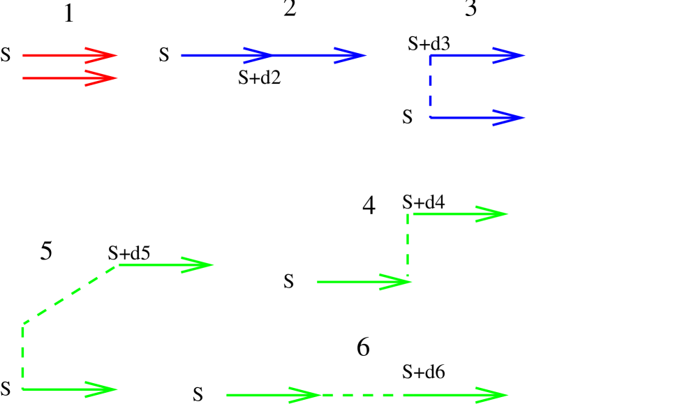
FIG. 1.: The first six terms of monopole interactions in the action.

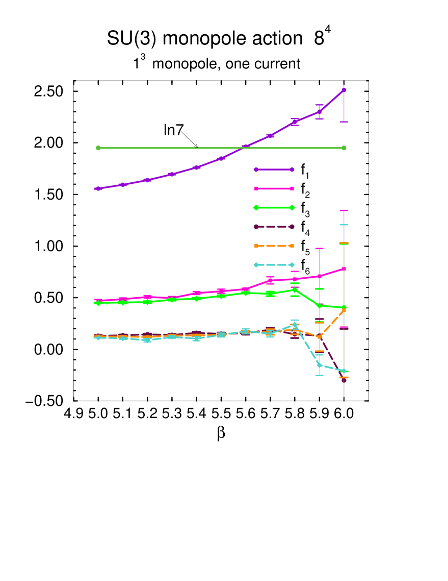
FIG. 2.: The effective monopole action in $T=0$ $SU(3)$ QCD.

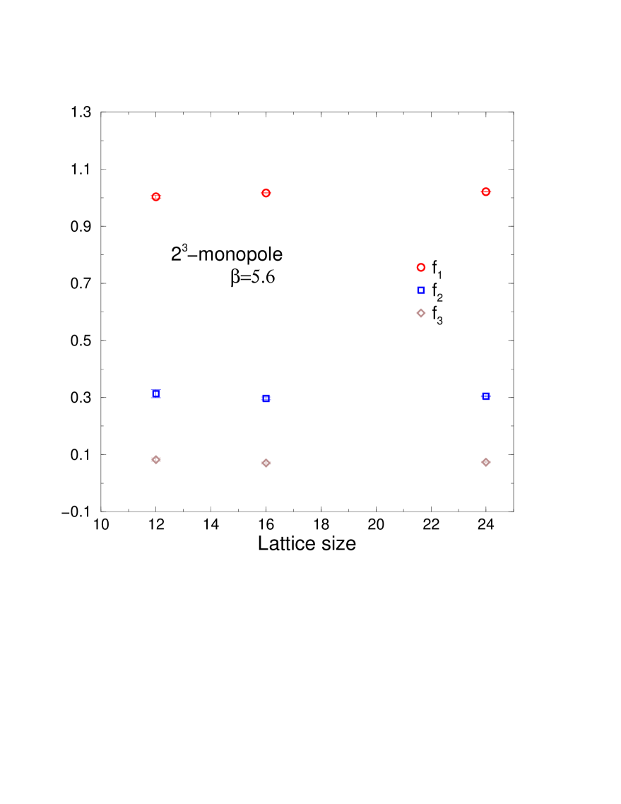
FIG. 3.: Coupling constants $f_{i}$ versus lattice size.

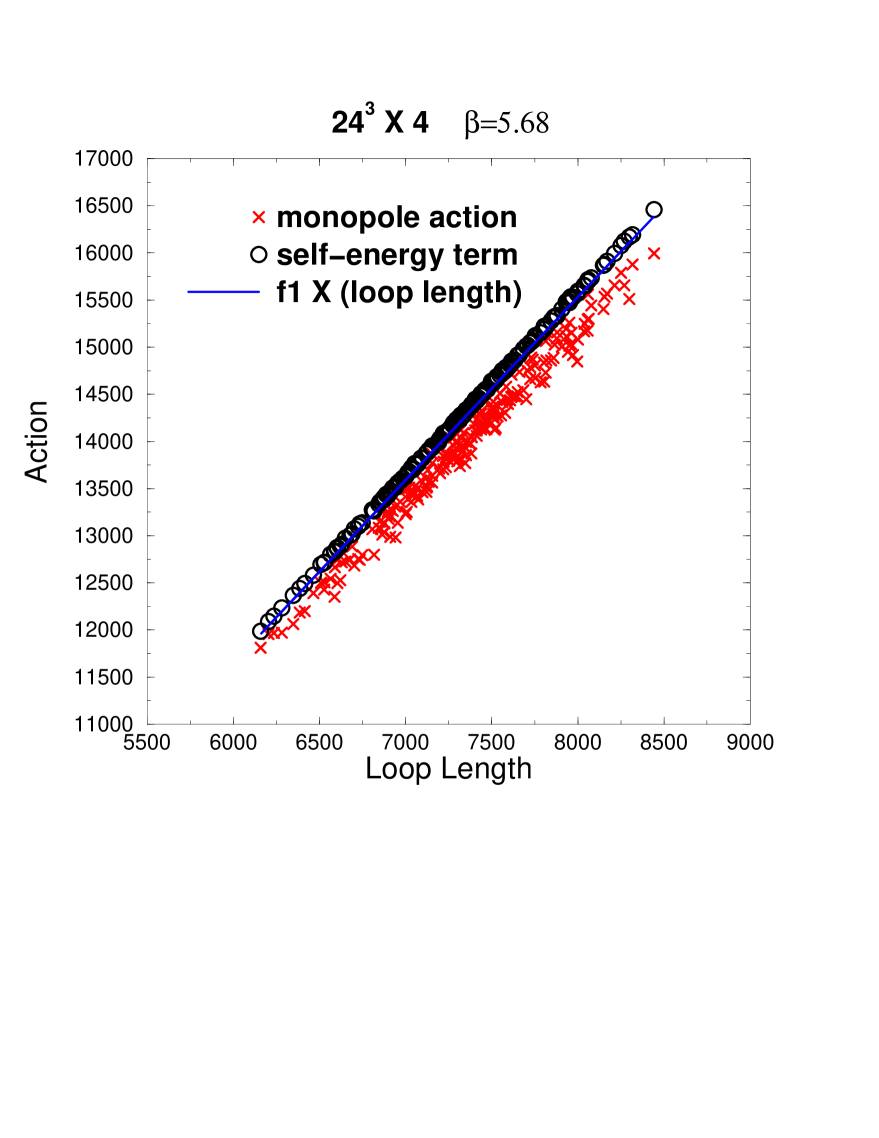
FIG. 4.: The total monopole action, the self-energy term of the action and $f_{1}$ times the length of a monopole loop $L$ versus length of the long monopole loop.

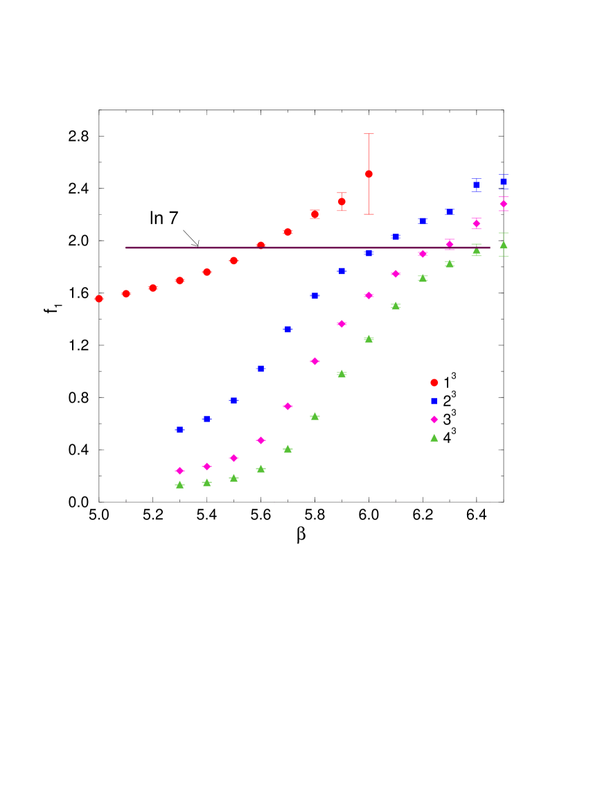
FIG. 5.: Coupling constants $f_{1}$ versus $\beta$ for $2^{3},3^{3}$ and $4^{3}$ extended monopoles on $24^{3}$ lattice.

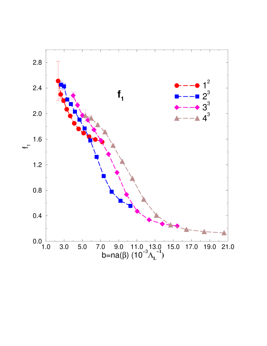
FIG. 6.: Coupling constants $f_{1}$ versus $b$.

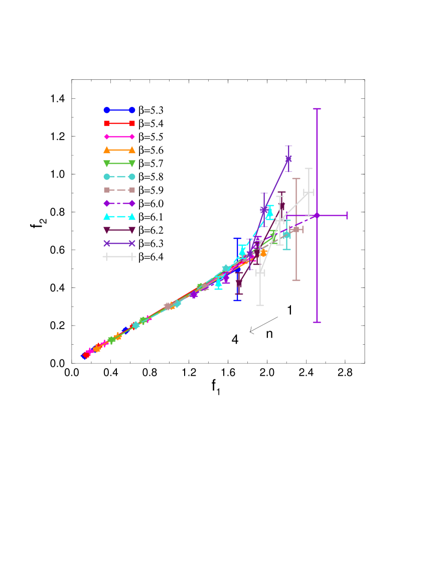
FIG. 7.: The $f_{1}-f_{2}$ plane of the renormalization flow.

FIG. 8.: The self-energy coupling constants for space-like monopole currents and for time-like monopole currents in the case of hot-start.

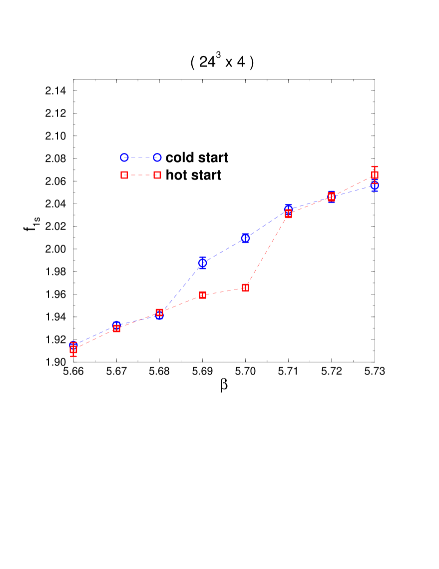
FIG. 9.: $f_{1}$ for the space-like currents near the transition temperature ($\beta_{c}=5.69$).

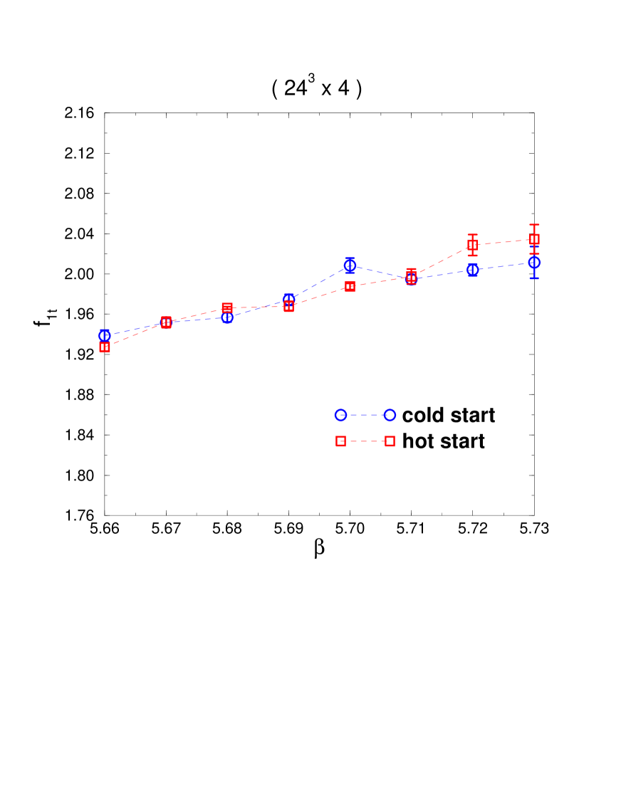
FIG. 10.: $f_{1}$ for the time-like currents near the transition temperature ($\beta_{c}=5.69$).

REFERENCES

- [1] G.’tHooft,High Energy Physics, ed.A.Zichichi (Editorice Compositori, Bologna, 1975).
- [2] S. Mandelstam, Phys. Rep. 23C (1976) 245.
- [3] A.M. Polyakov, Phys. Lett. 59B (1975) 82.
- [4] T.Banks , Nucl. Phys. B129 (1977) 493.
- [5] T.A. DeGrand and D. Toussaint, Phys. Rev. D22 (1980) 2478.
- [6] G. ’tHooft, Nucl. Phys. B190 (1981) 455.
-
[7]
A.S. Kronfeld , Phys. Lett.
198B (1987) 516,
A.S. Kronfeld , Nucl.Phys. B293 (1987) 461. - [8] T. Suzuki and I. Yotsuyanagi, Phys. Rev. D42 (1990) 4257; Nucl. Phys. B(Proc. Suppl.) 20 (1991) 236.
- [9] S. Hioki , Phys. Lett. 272B (1991) 326.
- [10] T. Suzuki, Nucl. Phys. B(Proc. Suppl.) 30 (1993) 176 and references therein.
- [11] R.M. Woloshyn, Phys. Rev. D51 (1995), 6411.
- [12] O. Miyamura, Nucl. Phys. B(Proc. Suppl.) 42 (1995) 538.
- [13] F.X. Lee et al., Nucl. Phys. B(Proc. Suppl.) 47 (1996) 561.
- [14] T.Suzuki et al., Nucl. Phys. B(Proc. Suppl.) 47 (1996) 374.
- [15] H.Shiba and T.Suzuki, Phys. Lett. 333B (1994) 461.
- [16] J.D.Stack, R.J.Wensley and S.D.Neiman, Phys.Rev. D50 (1994) 3399.
- [17] S. Ejiri et al., Nucl. Phys. B(Proc. Suppl.) 47 (1996) 322.
- [18] S. Ejiri, Nucl. Phys. B(Proc. Suppl.) 47 (1996) 539.
- [19] M.E. Peshkin, Ann. Phys. 113, (1978) 122.
- [20] J. Frölich and P.A. Marchetti, Euro. Phys. Lett. 2, (1986) 933.
- [21] J. Smit and A.J. van der Sijs, Nucl. Phys. B355, (1991) 603.
- [22] H.Shiba and T.Suzuki, Kanazawa University, Report No. Kanazawa 94-11, 1994.
- [23] H.Shiba and T.Suzuki, Kanazawa University, Report No. Kanazawa 93-09, 1993.
- [24] H.Shiba and T.Suzuki, Nucl. Phys. B(Proc. Suppl.) 34, (1994) 182.
- [25] H.Shiba and T.Suzuki, Phys. Lett. B351 (1995) 519.
- [26] T.Suzuki et al., Nucl. Phys. B(Proc. Suppl.) 47 (1996) 270.
- [27] R.H. Swendsen,Phys. Rev. Lett. 52, (1984) 1165; Phys. Rev. B30, (1984) 3866, 3875.
- [28] T.L. Ivanenko , Phys. Lett. 252B, (1990) 631.
- [29] T.Suzuki et al., Talk at ’Lattice 96’. To be published in Nucl. Phys. B(Proc. Suppl.).
- [30] F. Brandstaeter et al., Phys. Lett. B272 (1991) 319.
- [31] H.Shiba and T.Suzuki, Phys. Lett. B343 (1995) 315.
- [32] S. Kitahara, Y. Matsubara and T. Suzuki, Prog. Theor. Phys. 93 (1995), 1.