Improved lattice actions

Abstract

The main strategies to reduce lattice artifacts for spin models, gauge fields, free fermions and QCD are discussed.

1 INTRODUCTION

The idea to improve lattice actions [1, 2] is nearly as old as the use of lattices in regularizing field theories [3]. Nevertheless, until recently numerical simulations were performed mostly with the simplest (standard) form of lattice actions. This attitude seems to have been altered — at this conference there were probably more contributions using some kind of improved action than the standard ones. The reason is, obviously, that the lattice artifacts resulting from the finite lattice spacing $a$ cannot be easily reduced further simply by brute force, i.e. increasing the lattice size. As explained in Ref. [4] the computing cost for full QCD grows at least as $1/a^{6}$. I would like to add to this that in some cases the situation is much worse, even for pure gauge theory.

• Thermodynamics.
  For measuring the basic thermodynamic quantities, like the free energy, a conservative estimate gives

  $$\mbox{computing cost~{}}\sim\frac{1}{a^{10}}.$$

  (This is because the free energy density, $f={\rm O}(T^{4})$, is hidden behind the ultra–violate fluctuations of the action density, $\langle S\rangle={\rm O}(1/a^{4})$, as will be discussed later.)

• Topological susceptibility.
  Using the standard form of the action (with the geometrical definition of the topological charge) the presence of dislocations — configurations with topological charge and too small value of the action – spoil the result even in the continuum limit $a\to 0$!

In this talk I will concentrate mostly on theoretical ideas and developments, since the numerous contributions concerning simulations with improved actions are covered in several plenary talks at this conference.

2 IMPROVING THE ACTIONS

There are two main ways of improving the lattice actions, based on:

• Wilson’s renormalization group (RG),

• Symanzik’s approach, inspired by perturbation theory (PT).

Wilson’s approach [1] is based on the fact that a critical system (with a correlation length $\xi=\infty$) remains critical after mapping the lattice to a coarser one by a block transformation. The lattice action itself changes, in general, under the renormalization group transformation (RGT) and moves (except for pathological transformations as decimation) towards a fixed point (FP) on the critical surface. The trajectory leaving the critical surface along the relevant (unstable) direction(s) defines the renormalized trajectory. The system specified by an action on the renormalized trajectory has exactly the same partition function as the original system defined on an ‘infinitely fine’ lattice, and describes the same long–range physics with no lattice artifacts. The RGT can be (to a large extent) arbitrary, leading to different FP’s and renormalized trajectories. There is, however, an additional useful option — one can vary (and optimize) the RGT during the successive RG steps on the way to smaller and smaller correlation length. One can call this a ‘running’ RGT. The actions in this large set have the property that they are perfect – i.e. produce no cut–off effects (for physical quantities like masses, scattering amplitudes).

The disadvantage of this beautiful construction is that the actions involved have complicated structure, and it is difficult to determine and use them in numerical simulations. Perhaps to avoid these difficulties, Symanzik [2] suggested an alternative approach. The procedure was to add some extra terms to the naive lattice action and choose their coefficients appropriately to cancel the leading O($a^{2}$) lattice artifacts in the n-point Green–functions up to a given order in PT. (O($a^{2}$) refers to the bosonic case; for Wilson fermions the leading artifacts are more severe, O($a$)). For gauge theories this requirement had to be reduced to ‘on–shell improvement’, i.e. to the perturbative improvement of physical quantities [5, 6]. The number of extra terms to be added is determined by the number of possible ${\rm dim}=(5),6$ operators. By allowing redefinitions of fields, however, this number can be reduced. The number of extra operators to be added is following:

	op’s	order	Ref.
gauge fields:	3-1=2	O($a^{2}$)	[5, 6]
fermions	2-1=1	O($a$)	[7]
	15-5=10	O($a^{2}$)	[7]

(Some of the 10 fermionic operators contributing to O($a^{2}$) are quartic in the fermion fields.) The statement is that to arbitrary order in $g^{2}$ only the coefficients of these operators have to be determined to cancel the corresponding cut–off dependence of O($g^{n}a$) or O($g^{n}a^{2}$). Although the Symanzik approach provides a relatively simple modification of the action to cancel the leading artifacts, the perturbatively determined coefficients are usually not applicable in the case where most of the numerical simulations are done. The other point, to which I shall return, is that there is a large freedom of choosing the given number of extra operators, and some additional criteria are needed to find the choice best suited for numerical simulations.

3 RECENT DEVELOPMENTS

I will consider three main recent developments in the improvement program:

• non–perturbative numerical determination of O($a$) improvement coefficients in QCD [8]

• tadpole improvement (TI) [9, 10]

• FP actions (or classically perfect actions) [11, 12, 13, 14, 20]

The first one is a direct application of Symanzik’s improvement program for the non–perturbative situation in QCD: instead of calculating the O($a$) cut–off effects for some quantities in PT, the authors measure these effects, and by tuning the coefficient $c_{SW}(g_{0}^{2})$ of the Sheikholeslami–Wohlert (clover) term [7] they get rid of the leading O($a$) artifacts. Since it is done in the framework of the full QCD, I will discuss it at the end, and start with the simpler case of bosonic theories.

4 TADPOLE IMPROVEMENT

The motivation behind this approach is the observation that large coefficients appearing in PT come dominantly from tadpole diagrams. Lepage and Mackenzie suggested [9] that these contributions should be removed by a mean–field redefinition of the original fields. The corresponding prescription for the SU(3) gauge fields is to replace the fields in the original lattice action according to the rule

$$U_{\mu}(x)\to\frac{1}{u_{0}}U_{\mu}(x)\,,$$ (1)

where

$$u_{0}=\langle\frac{1}{3}{\rm Tr}U_{\rm plaq}\rangle^{1/4}\,.$$ (2)

In addition, to get a better perturbative expansion, it is suggested to use

$$\alpha_{s}=-\frac{1}{3.06839}\log\left(\frac{1}{3}\langle U_{\rm plaq}\rangle\right)$$ (3)

as an expansion parameter instead of $\alpha_{\rm latt}=g_{0}^{2}/4\pi$.

For tadpole improving (TI) a one–loop Symanzik improved (SI) action (where the coefficients are $g$ dependent) the prescription is to recalculate the improvement coefficients for the modified action obtained by (1) using ordinary PT, substitute $\alpha_{\rm latt}\to\alpha_{\rm s}$, and use this action in the numerical situation. The procedure involves a self–consistent determination of the coefficients in the action: the coefficients to be used in the MC simulation have to be determined from MC simulations. Technically, this is not a serious problem, since it is very easy to measure $\langle U_{\rm plaq}\rangle$. (Principally, however, the mean field definition can cause some problems. For example, $\langle U_{\rm plaq}\rangle$ depends not only on $\beta$ but also on the size of the system. Should one change $u_{0}$ with the temperature at a given $\beta$ according to eq. (2) or should it be determined from the zero temperature, infinite volume case? One can argue both ways.)

I cite here two examples of tadpole improvement. For the O($a$) one–loop Symanzik–improved Wilson fermions the coefficient [15, 16, 17]

$$c_{SW}=1+0.2659g_{0}^{2}+\ldots$$ (4)

should be compared with the TI tree–level Symanzik–improved action which gives

$$c_{SW}^{(0)TI}=\left(\frac{1}{3}{\rm ReTr}\langle U_{\rm plaq}\rangle\right)^{-3/4}=1+0.25g_{0}^{2}+\ldots$$

In other words, 94% of the original one–loop correction is removed by making the TI in the tree–level formula. Accordingly, tadpole improving the 1-loop formula amounts to using $c_{SW}^{TI}=1+4\pi\cdot 0.0159\alpha_{s}$. For the pure gauge field TI for the 1-loop SI action of Lüscher and Weisz [6] (who have used the plaquette (pl) and the rectangle (rt) ) means

$$\frac{\beta_{\rm rt}}{\beta_{\rm pl}}=-\frac{1}{20}(1+2.0146\alpha_{s})\to-\frac{1}{20u_{0}^{2}}(1+0.4805\alpha_{s})$$

i.e. 76% of the coefficient has been removed by applying (1) to the tree–level result.

The TI action for gauge fields has been demonstrated to work well even for lattices as coarse as $a\sim 0.4{\rm fm}$ [4]. This success and the simplicity of the prescription resulted in a large number of contributions to this conference which apply TI actions in numerical simulations. However, as we shall discuss later, TI does not work everywhere, e.g. for full QCD it does not give properly the value of $c_{SW}$ at the $\beta$ values of interest [8].

After discussing the FP actions, I will try to suggest how to understand the tadpole improvement from the corresponding point of view.

5 FIXED POINT ACTIONS

To be specific, I will consider here the pure gauge theory. A RGT is defined by specifying the kernel of the block transformation, $T(V,U)$. Here $V$ is a gauge configuration on the coarse lattice while $U$ denotes a configuration on the fine lattice. Given the action $S(U)$ one defines $S^{\prime}(V)$ by

$${\rm e}^{-\beta^{\prime}S^{\prime}(V)}=\int dU{\rm e}^{-\beta[S(U)+T(V,U)]}\,.$$ (5)

($S^{\prime}(V)$, as well as $S(U)$, is normalized to the continuum expression for very smooth fields.) $T(V,U)$ should satisfy a normalization condition to leave the partition function unchanged. Since the theory is asymptotically free, for $\beta\to\infty$ one has $\beta^{\prime}=\beta+{\rm O}(1)$, and in this limit eq. (5) reduces to a saddle point equation:

$$S^{\prime}(V)=\min_{U}\left\{S(U)+T(V,U)\right\}\,.$$ (6)

The fixed point of this transformation is given by

$$S^{\rm FP}(V)=\min_{U}\left\{S^{\rm FP}(U)+T(V,U)\right\}\,.$$ (7)

Note, that although the $\beta\to\infty$ limit has been taken, the fields $V$ and $U$ are not assumed to be necessarily smooth — they could be arbitrarily rough as well in this definition. Eq. (7) can be solved analytically for smooth configurations and numerically for arbitrary $V$ by iteration. The iterative procedure converges very rapidly since the typical action density on the fine lattice is $\sim 30$ times smaller than that on the coarse lattice (a factor 16 coming from the volume, and typically half of the value of the r.h.s. is due to $T(V,U)$.) Consequently, in most cases one can use on the r.h.s. just the quadratic approximation to $S^{\rm FP}(U)$ or even the standard action.

The FP action has remarkable properties — it defines a classically perfect lattice action [18], in the following sense. The solutions to the lattice equations of motion are related to their continuum counterparts, with the same value of the action:

$$S_{\rm cont}(U_{\rm cont})=S_{\rm latt}^{\rm FP}(U_{\rm latt})\,.$$ (8)

In particular, for continuum theories possessing instantons, the FP action has scale invariant instanton solutions as well. One can say that the FP action is ‘tree–level Symanzik–improved to all orders in $a$’. By proper choice of $T(V,U)$ (which is achieved by tuning some free parameters in it) $S^{\rm FP}$ can be made quite short ranged — the couplings outside the unit hypercube can be suppressed (relative to the plaquette) by a factor $\sim 100$ [11]. The FP action is not expected to be a perfect action — using it in numerical simulations with finite $\beta$ (at finite correlation length) some cut–off dependence remains. Numerical simulations for $2d$ spin models [18, 19, 20] and $4d$ SU(3) gauge theory [11] show, however, that the lattice artifacts using FP actions are negligible for these theories even on extremely coarse lattices.

Actions which are (quantum) perfect are obtained by following the renormalized trajectory (also allowing to vary $T(V,U)$ with $\beta$). Strong arguments suggest that the FP action is also 1–loop perfect, i.e.

$$\beta S^{\rm perf}(U;\beta)=\beta S^{\rm FP}(U)\left[1+{\rm O}\left(\beta^{-2}\right)\right]\,.$$ (9)

This conjecture is supported by formal RG arguments [1, 11] and by numerical evidence for the O(3) non–linear sigma–model [21]. In [21] it was found that the mass gap in a small box calculated to 1–loop in PT with the FP action has no O($g^{4}a^{n}$) error. A coefficient $R$ appearing in the 1–loop expansion of the mass gap is plotted vs. $(a/L)^{2}$ in Fig. 1. As seen, the correction is vanishing as $\exp(-\gamma L/a)$. This reflects the requirement that the size of the box should be larger than the interaction range of the FP action (otherwise the infinite–volume action should be modified). The tiny power–like artifact seen in the fit is caused by restricting the interaction distances considered in the perturbative calculation.

Figure 1: The value of $R$ vs. $(a/L)^{2}$ for the FP action for $L/a=2,3,\ldots,10$. The fit shown is $-0.1422022-0.0000176\,(a/L)^{2}$. Note that the exact limiting value is $-0.1422024$.

Although the FP action is classically and presumably 1–loop perfect, the approximation actually used in MC simulations contains some imperfect steps:

• truncation in the interaction distance,

• parametrization (choice of the set of operators to fit the numerically known values of the FP action)

• the FP action is not on the renormalized trajectory (it is not ‘quantum perfect’).

One has to control these points to get a reliable FP action. It produces a misleading result, for example, to restrict the RGT to a small subspace of operators beforehand. One must show first that the interaction range is not larger than the truncation radius for the interaction terms and truncate the set of operators only afterwards.

5.1 Natural choice of improvement terms

In Symanzik’s approach one has a large freedom to choose the improvement terms. For the tree–level improvement to ${\rm O}(a^{2})$ one can choose the following loops, for example,

1. the plaquette and the rectangle ($2\times 1$ loop),

2. the plaquette and the $2\times 2$ loop.

Which one should be preferred? Let me illustrate the point on the $2d$ $\sigma$–model. Denote by $\rho_{xy}$ the coupling between two spins at the relative distance $(x,y)$. (The standard action is given by the nearest–neighbour term $\rho_{10}=1$.) Take two choices of operators in the Symanzik approach:

1. $\rho_{10}=4/3$, $\rho_{20}=-1/12$,

2. $\rho_{10}=2/3$, $\rho_{11}=1/6$,

The FP values for these coefficients (for an ‘optimal’ RGT [18]):

$$\rho_{10}=0.618,~{}\rho_{11}=0.190,~{}\rho_{20}=0.002$$

The choice a.) has an antiferromagnetic coupling and a complex dispersion relation in the quadratic approximation. Clearly, our RGT prefers the choice b.) in the Symanzik program, which is free from these diseases.

Similarly, for gauge theory the FP action in quadratic approximation gives a much smaller coefficient for the rectangle (rt) than for the ‘bent rectangle’ (brt) or the parallelogram (pg) [11]. (Note that the brt and pg are equivalent in the quadratic approximation.) In the standard tree–level SI form, however, the plaquette (pl) and the rt are the two operators chosen to have non–zero coefficients. This choice does not correspond to the FP action. In quadratic approximation it produces again a complex spectrum above some momenta. In fact, Lüscher and Weisz [6] proposed a one–parameter family of SI actions with a free coefficient $x$ for the brt, suggesting that $x\neq 0$ could be useful in MC simulations. However, as far as I know, only the $x=0$ choice has been exploited.

I think, for the Symanzik program a natural choice of the improvement operators could be the one inspired by the RG approach. One can also turn the argument around. As mentioned above, the FP action is automatically Symanzik–improved, to all orders in $a$. A necessary truncation to a reasonable number of operators does not keep, of course, this property. Nevertheless, for a FP action with a short interaction range the violations of the lowest order (in $a$) Symanzik conditions will be small. Since the truncation is to some extent an arbitrary procedure, one might also keep these conditions satisfied. I note here, that we were interested mainly in a good parametrization of the FP action at relatively rough configurations (typical at short correlation length) hence we did not always impose the above conditions.

5.2 Parametrization of the FP action

In [11] the FP action has been parametrized as

$$S^{\rm FP}(U)=\sum_{\cal C}\sum_{m}c_{m}({\cal C})X_{\cal C}^{m}\,,$$ (10)

with

$$X_{\cal C}={\rm ReTr}\left(1-U_{\cal C}\right)\,,$$ (11)

and ${\cal C}$ denotes a closed loop. A few simple loops were taken with their powers $m=1..4$. The higher powers are essential in this parametrization, and they do not cause much overhead in numerical simulations. With a Swendsen-type blocking in ref. [11] a good scaling was observed for $a\leq 0.4{\rm fm}$. In addition, a good asymptotic scaling for $T_{c}/\Lambda$ has been found, which could indicate that the bare PT for the FP action works better.

On the renormalized trajectory the coefficients in eq. (10) will be $g$ dependent. The 1–loop perfectness, however, predicts that this dependence is given by

$$c_{m}({\cal C},g)=c_{m}({\cal C})+{\rm O}(g^{4})\,,$$ (12)

i.e. no O($g^{2}$) corrections are expected. One concludes that no large tadpole contributions could be present for the FP action, and it would be incorrect to tadpole improve it by

$$S^{\rm FP}(U)\to S^{\rm FP}(U/u_{0})\,.$$ (13)

On the other hand, a mean field approximation to the FP action (10) yields an action of the TI type:

$$S^{\rm FP}\approx\sum_{\cal C}c_{\rm eff}({\cal C},\langle X_{\cal C}\rangle)X_{\cal C}\,,$$ (14)

where $c_{\rm eff}({\cal C},\langle X_{\cal C}\rangle)=c_{1}({\cal C})+2c_{2}({\cal C})\langle X_{\cal C}\rangle+\ldots$ Indeed, the relative weight of the parallelogram (pg) to the plaquette, $c_{\rm eff}({\rm pg})/c_{\rm eff}({\rm pl})$ grows with $g^{2}$ as suggested by the tadpole improvement (where it is $\propto 1/u_{0}^{2}$).

5.3 Improving correlators of local operators; the $q\bar{q}$ potential

In the Symanzik approach one improves the action to cancel cut–off effects in spectral quantities. To achieve this for correlation functions one also has to improve the operators. The situation is the same in the RG approach. For a square–shaped blocking, although the spectrum is exact, the potential shows violations of rotational symmetry. (A close analogy: in the continuum electrodynamics the interaction between square–shaped charges.) The perturbative $q\bar{q}$ lattice potential has, in general, terms of the following type:

$$V(r)\sim\frac{1}{r}+\ldots\frac{a^{2}}{r^{3}}+\ldots\frac{a^{4}}{r^{5}}{\rm P}_{4}(\cos\theta)+\ldots{\rm e}^{-\gamma r/a}\,.$$

The second term (related to the distorted gluon spectrum) is removed by improving the action, the third one (an octupole term) by improving the operator. In the RG approach, the last term comes from the interaction of the quantum fluctuations on the fine lattice for a given coarse configuration (and is similar in nature to the exponentially vanishing term in Fig. 1). In Ref. [11] using a Swendsen–type RGT (our type–1 RGT) we have got a $q\bar{q}$ potential which gave the proper string tension at $a=0.4{\rm fm}$ but had considerable violation of rotational symmetry at small distances. This has been associated in ref. [11] with the strongly square–shaped averaging of the RGT applied. To illustrate this point, and also to obtain an even better FP action, in Ref. [22] a more general RGT (type–3) has been considered, which included generalized staples along the $2d$ and $3d$ diagonals. As expected, the rotational invariance at small distances has been improved both for the perturbative and the non–perturbative potential. In Fig. 2 the deviation of the perturbative potential from the continuum result is shown. In Fig. 3 the $q\bar{q}$ potential measured at finite temperature $T=2/3\cdot T_{c}$ and $a\approx 0.4{\rm fm}$ is compared for the Wilson action and type–3 FP action [22]. For comparison, I measured also the 1–loop tadpole–improved potential for this temperature, also shown in Fig. 3. Surprizingly, the tadpole and the type–3 FP data almost coincide.

Figure 2: The difference $V(r)-V_{\rm cont}(r)$ vs. $r$ for the Wilson action, type–1 and type–3 FP actions.

Figure 3: $V(r;T)/T_{c}$ vs. $rT_{c}$ for the Wilson, type–3 FP and 1–loop TI actions, at finite temperature, $T=2/3\cdot T_{c}$. The dashed line is the universal curve.

Although it is not related to the FP actions, I end this section with a reference to [23] where it has been suggested to test improvement schemes by using analytic and numerical methods in a small physical volume. The authors proposed a combination of the plaquette, the $2\times 1$ and the $2\times 2$ loops, with coefficients $16/9$, $-1/9$ and $1/144$ which also satisfy the tree–level Symanzik conditions. The improvement for the small volume quantities is about the same as for the Lüscher–Weisz choice ($5/3$, $-1/12$ and $0$). The choice of [23] is motivated by the observation that their analytic calculations could be extended to investigate the effects of the TI in this case.

Let me also mention a contribution [24] where the authors used the 1–loop SI + TI gauge action on anisotropic lattices to calculate the glueball mass. The use of an anisotropic grid which is finer in the time direction ($a_{t}<a_{s}$) is a useful tool to study heavy objects. The data for the $0^{++}$ and $2^{++}$ glueballs scale well up to $a_{s}=0.4{\rm fm}$, while the standard action shows large artifacts on coarse lattices.

6 THERMODYNAMICS

Thermodynamic quantities measured at relatively large temperatures are sensitive not only to the low energy part of the spectrum hence the lattice artifacts in this case are usually much larger. For example, in PT for $T\to\infty$ at temporal lattice size $N_{t}=4$ the cut–off effect for $p/T^{4}$ using Wilson’s gauge action is $\approx 50\%$ [25].

The pressure is given by

$$\left.\frac{p}{T^{4}}\right|_{\beta_{0}}^{\beta}=N_{t}^{4}\int_{\beta_{0}}^{\beta}d\beta^{\prime}\left(\langle S\rangle_{0}-\langle S\rangle_{T}\right)\,.$$ (15)

Here the action densities on the r.h.s. are measured at a given $\beta^{\prime}$ for two different temporal geometries, at $N_{t}=\infty$ (or rather for a 4–cube $N_{t}=N_{s}$) and $N_{t}$ corresponding to the given temperature $T$. (Actually, this is the formula which shows that the corresponding computer cost grows like $N_{t}^{10}$, as mentioned in the introduction.) In Ref. [25] the authors measured $p/T^{4}$ with the standard action for $N_{t}=4,6,8$ and a few improved actions, including the $2\times 1$ 1-loop TI action for $N_{t}=4$. (For the results see the figure in Ref. [27].) Papa  [28] has measured the same quantity for the FP actions with RGT of type–1 and type–3, for $N_{t}=2,3$ and $T=2T_{c}$. The relative deviations from the continuum result (obtained by extrapolating the standard action results) for $T=2T_{c}$ are given below.

$N_{t}$	Wilson	type–1	type–3	tadpole
2	100%	25%	10%
3		10%	”0%”
4	20%			”0%”

”0%” means that no deviation is seen within the error. Note that the $N_{t}=2$ case is special because of possibly large $\exp(-\gamma N_{t})$ type corrections.

One can conclude that the cut–off effects are drastically reduced using these improved actions.

7 TOPOLOGICAL SUSCEPTIBILITY

The FP action is especially suited for measuring topological effects:

• it has scale invariant instanton solutions (for sizes $\rho\geq 0.7a$)

• a good definition of topological charge is possible (classically perfect $Q$)

Definition: Measure the topological charge on the minimized fine configuration $U=\overline{U}(V)$ of eq. (7),

$$\overline{Q}(V)=Q(\overline{U}(V))$$ (16)

(Here I mean a minimization iterated a few times if necessary, on even finer grids. Since on the fine grids the fields are rather smooth, after the second iteration the value of $Q$ usually does not change.) The charge $\overline{Q}(V)$ avoids the problem of dislocations: any configuration $V$ with $\overline{Q}(V)=1$ has a value of the FP action not smaller than the continuum result, $S^{\rm FP}(V)\geq S_{\rm cont}^{\rm inst}$.

By measuring the topological charge this way, one also avoids problems associated with the cooling procedure (e.g. the disappearance of the instantons) — the minimization procedure provides a prescription to separate the fluctuations from a smooth background solution. The configuration $\overline{U}(V)$ is smoother than $V$, it is closer to a solution — part of the energy of the fluctuations in $V$ is taken over by $T(V,U)$ in eq. (7). If $V$ is a solution then $T(V,\overline{U}(V))=0$. Consequently, the minimization $V\to\overline{U}(V)$ provides an ideal cooling procedure. A serious drawback is that the minimization procedure is very slow, it is hard to use it in a MC measurement. A solution is to find an approximate analytical form for the function $\overline{U}(V)$ as has been done for the spin models [19, 20].

This strategy has been applied to the 2d non–linear sigma–model [19], the 2d ${\rm CP}^{3}$ model[20], and to the 4d SU(2) gauge model [29]. For the O(3) model $\chi_{t}\xi^{2}$ does not scale (not unexpectedly) while the ${\rm CP}^{3}$ model shows a beautiful scaling, for $\xi\geq 7$. In addition, asymptotic scaling is found in $m/\Lambda_{\rm 2-loop}$ for $\xi\geq 4$, suggesting again that the bare PT should work better for the FP action. Of course, in the $4d$ SU(2) gauge theory the technical difficulties are more serious, and the investigations are not completed yet. Nevertheless, the results for the scaling of the topological susceptibility [29] are encouraging. For the corresponding plots see Ref.’s [20, 29].

Let me discuss a few points in some detail. Blocking down a smooth instanton solution to a coarser lattice remains an instanton solution until $\rho\sim 0.7a$ where $\rho$ is the size of the instanton. Instantons of smaller size ‘fall through the lattice’ — they cannot be distinguished from local excitations. This is the consequence of the classical (saddle point) approximation. By fixed coarse configuration $V$ at finite $\beta$ in eq. (5) the typical fine configuration $U$ fluctuate around the minimizing configuration $\overline{U}(V)$. These can have different charges, especially if the action density of $V$ is localized to a small region. In contrast, $\overline{U}(V)$ assigns a unique fine configuration to $V$, and for instantons which ‘fell through the lattice’ this gives zero topological charge. Hence the contribution of these small instantons is lost by using the FP action and FP topological charge on the coarse lattice. Nevertheless, the definition (16) of the FP–charge associates $\overline{Q}=0$ for these small size excitations so they don’t spoil the topological susceptibility. One expects to observe scaling of $\chi_{t}\xi^{d}$ once the role of instantons of size $\rho\leq 0.7a$ becomes negligible. By using the standard action and even the (tree-level or 1–loop) SI action, there is a wide range of instanton sizes where the instanton action is smaller than the continuum value while the charge associated is 1 in the geometrical definition — see the corresponding figure in Ref.[20]. As a consequence, one can grossly overestimate $\chi_{t}$ and observe scaling only at much finer lattices. I also have the feeling that using TI will not help much in this case — the mean field approximation represents the action at some average ‘roughness’ of the fields, while instantons of different sizes are perhaps important at a given value of $\beta$. In Ref. [14] the authors discuss the notion of the ‘quantum perfect topological charge’ on the example of the exactly soluble 1d XY–model.

Note that the use a parametrized form for the minimized fine field $\overline{U}(V)$ technically might be similar to applying appropriately smeared fields to measure the topological charge [30].

8 NON–PERTURBATIVE DETERMINATION OF IMPROVEMENT COEFFICIENTS

In QCD with Wilson fermions the Wilson term (which has been introduced to avoid the doubling problem) explicitly breaks chiral invariance and induces ${\rm O}(a)$ cut–off effects in chiral relations. To remove these artifacts it has been proposed to modify the fermion action by a Pauli term $ac_{\rm SW}\bar{\psi}\sigma_{\mu\nu}\psi F_{\mu\nu}$. The lattice representation of this operator is chosen to be the ‘clover’ term [7]. The coefficient $c_{\rm SW}(g_{0})$ has been determined in the SI approach to 1–loop order and given by eq. (4) [15, 6]. In Ref. [8] the dependence of this coefficient on the coupling $g_{0}$ has been determined by non–perturbative methods. The framework used was the Schrödinger functional method, where instead of periodic boundary conditions in the time direction Dirichlet b.c.’s are used for the gauge fields and fermions. This has the advantage that a background field can be introduced in the system and the response to this field can be investigated. By using a small physical box and Dirichlet b.c. the zero modes in the fermion matrix are avoided, hence this framework is especially suited to study the chiral limit $m\to 0$.

From the PCAC relation $\partial_{\mu}A_{\mu}^{a}(x)=2mP^{a}(x)$ for the axial current and pseudoscalar density, valid in the continuum limit, the authors define

$$m=\frac{\langle\partial_{\mu}A_{\mu}^{a}(x){\cal O}^{a}\rangle}{\langle P^{a}(x){\cal O}^{a}\rangle}\,,$$ (17)

where ${\cal O}^{a}$ is a fermionic operator on the boundary. For Wilson fermions this quantity depends very strongly on the position $x$ and the background field, even at $a=0.05{\rm fm}$! Introducing the SW term into the action, and an extra term in the current via

$${\cal A}_{\mu}^{a}(x)=A_{\mu}^{a}(x)+c_{A}a\partial_{\mu}P^{a}(x)\,,$$ (18)

by properly tuning the coefficients $c_{\rm SW}$ and $c_{A}$ one can make the quantity (17) independent of $x$ and the background field. Fig. 4 shows the dependence of $c_{\rm SW}$ on the coupling [8].

Figure 4: Dependence of $c_{\rm SW}$ on the coupling,

We can conclude that the SW choice for the improvement term works well, but the coefficient is strongly non–perturbative in the interesting region of couplings. Perhaps one can try other schemes where the higher order (or non–perturbative) corrections are smaller. Note also that the tadpole improvement of the 1–loop SI result at $\beta=6$ fails by about 15% and the discrepancy seems to grow rapidly with $g_{0}$.

In a work presented at this conference [31] Göckeler et al. used the value $c_{\rm SW}$ predicted by the ALPHA collaboration [8]. Their results at $\beta=6$ shown on an APE plot seem to extrapolate well to the physical ${\rm N}/\rho$ ratio. R. Gupta noted that minimizing the source–dependence in his measurements prefers a value of $c_{\rm SW}(g_{0})$ consistent with the ALPHA result [32].

9 FERMIONS

For fermions, compared to pure gauge fields, the cut–off effects are larger and the computational cost grows faster with the lattice size, hence it is especially important to optimize the choice of the lattice action used.

9.1 D234$\left(\frac{2}{3}\right)$ action

In their contribution to this conference, Alford, Klassen and Lepage [10] suggested a modification of the ‘D234’ fermionic action [33] which they call ‘D234$\left(\frac{2}{3}\right)$’. It is constructed using higher order lattice derivatives along the axis. In addition the authors also introduce anisotropic lattices, by taking different lattice spacings along the spatial and time directions, $a_{s}/a_{t}\sim 2~{}-~{}3$. With this additional trick the dispersion relation for free fermions becomes real and reasonably good. (For the isotropic lattice the dispersion relation is complex above $ap\approx 1$.) Note that the anisotropic choice, besides curing the spectrum has the advantage that one can measure time correlations on a finer scale which can be important for heavy objects. The authors have plotted the ‘velocity of light’ $c({\bf p})$, defined via $E({\bf p})^{2}=E(0)+c({\bf p})^{2}{\bf p}^{2}$, measured for different actions in the quenched approximation for $\pi$ and $\rho$. While the TI of 1–loop SI gluon+fermion action gives a large deviation from 1, the ‘D234$\left(\frac{2}{3}\right)$’ action on an anisotropic lattice produces good agreement with $c({\bf p})=1$.

I would like to point out that choosing an anisotropic lattice can be a useful tool in itself for dealing with heavy objects, but it is not needed to improve the spectrum of free fermions. As investigations of the FP fermionic actions show this goal can be achieved by using appropriate couplings on the unit hypercube.

9.2 FP actions for fermions

The RG approach to the fermion problem is presented at this conference by two groups, from MIT [14] and from Bern/Boulder [12]. The approaches of the two groups are very similar, the main difference is in the type of the blocking transformation used. This difference is of technical nature, the results obtained and the expectations are very similar.

The FP action for the massless free fermions has the form

$$S_{\rm F}^{\rm FP}=\sum_{n,r}\bar{\psi}(n)\left[\gamma_{\mu}\rho_{\mu}(r)+\lambda(r)\right]\psi(n+r)\,.$$ (19)

The features of this FP actions are:

• The spectrum is exact, there are no ${\rm O}(a^{n})$ cut–off effects (‘classically perfect’)

• There are no doublers, but chiral symmetry is violated. This violation is, however, very special: it comes entirely from the blocking transformation which is not affecting the physics.

• By optimizing the corresponding RGT the interaction range could be made quite small — couplings decrease exponentially fast and outside the unit hypercube could perhaps be neglected.

The $m\neq 0$ case is very similar, only in this case one does not have a FP, of coarse, since the mass is running. It is possible to start with an arbitrarily small mass and make an appropriate number of blocking transformations, doubling the mass in each step, until the given value of $ma$ is reached. An important point here is the following: the RGT which was optimal for the $m=0$ case will not be optimal for the massive case — by applying a fixed RGT the interaction range would grow. To stay with a short ranged action one has to modify the parameters of the RGT with the growing mass. This can be done for all RGT’s considered, and one can keep the action short ranged — at least up to $ma\approx 2$ but perhaps even higher.

In numerical simulation one needs to truncate the interaction distance $r$ in eq. (19). This introduces some imperfectness: the spectrum is distorted, ‘ghosts’ (higher lying and sometimes complex branches in the spectrum) appear, Symanzik’s improvement conditions for the spectrum will be (slightly) violated. Nevertheless, since by the truncation one neglects only small coefficients, these effects are not expected to be large. Table 1 lists some of the coefficients of a FP action (corresponding to one of the Bern/Boulder RGT’s) for free massless fermions. The coefficients $\lambda(r)$ and $\rho_{1}(r)$ decrease rapidly with the distance $r$ hence truncation to the unit hypercube seems to be justified.

$r$	$\lambda(r)$	$\rho_{1}(r)$
0000	$~{}2.312461$
1000	$-0.112098$	$0.140881$
1100	$-0.034557$	$0.034424$
1110	$-0.014912$	$0.010742$
1111	$-0.007373$	$0.003714$
2000	$~{}0.001493$	$0.001380$
3000	$-0.000088$	$0.000243$
4000	$~{}0.000000$	$0.000010$

Table 1: Some coefficients of a fermionic FP action.

Fig. 5 shows the spectrum $E(q,0,0)$ (along the axis) at $ma=0.005$ (for the fermionic action with this small mass and corresponding to the same RGT as above), as a typical example. The solid line is the exact spectrum, the dashed is for the action truncated to the hypercube, the long–dashed is the truncated one with tiny corrections to satisfy the Symanzik condition, the dot–dashed is for the Wilson fermions. Fig. 6 shows the same quantities for $m=1.28$. (Note that the Fermilab action [10] on the isotropic lattice gives a far worse dispersion relation: for $m=0$ it is complex and for $ma>0$ the kinetic mass is too small, see a figure in Ref. [14]. Remember, however, that it is assumed to be used on anisotropic lattices.)

Figure 5: Fermion spectrum at $ma=0.005$.

Figure 6: Fermion spectrum at $ma=1.28$.

The spectrum of the full FP action is, of course, exact for any value of the fermion mass (or rather $ma$). The coefficients $\rho_{\mu}$ and $\lambda$ in eq. (19) depend on the mass, and they decay exponentially in the distance $r$ as $\propto\exp(-\gamma r)$. A truncation at some small distance should necessarily induce ‘ghosts’ in the spectrum (higher branches, which are artifacts) with an energy $\sim\gamma$. A truncation is sensible therefore only if $ma<\gamma$. It is not yet clear what is the largest mass this condition allows ($\gamma$ will also depend on $ma$), but $ma\approx 2$ is still definitely allowed. To study higher lattice masses, one might need to consider anisotropic lattices, anyhow.

The mass dependence of the coefficients in eq. (19) follows a smooth curve which could be parametrized easily. In Fig. (7) the ratios $\lambda(r,ma)/\lambda(r,0)$ and $\rho_{1}(r,ma)/\rho_{1}(r,0)$ are shown for different $r$ values on the hypercube, only as an illustration to this statement. (Note that this dependence is obtained by an optimized ‘running RGT’.)

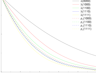
Figure 7: Mass dependence of the ratios $\lambda(r,ma)/\lambda(r,0)$ and $\rho_{1}(r,ma)/\rho_{1}(r,0)$.

As we saw, thermodynamic quantities are very sensitive to the cut–off effects. In Fig. 8 for the case of massless fermions the ratio $p/T^{4}$ is plotted vs. $N_{t}$, for the Wilson action, the full FP action and the FP action truncated to the unit hypercube (but still uncorrected for the tiny violation of the Symanzik condition). Note that the full FP action has a correction vanishing exponentially with increasing $N_{t}$.

Figure 8: $p/T^{4}$ vs. $N_{t}$ for massless fermions.

9.3 Fermions and gauge fields

The final goal of the improvement approach is to produce a good action of the full QCD. This goal is not achieved yet, but some important steps are already made. I shall review here the situation within the RG approach. To derive the FP action for the case of fermions + gluons the following steps have to be performed:

1. Find the FP action for the pure gauge fields and free fermions, eqs. (7,19), and obtain the corresponding minimized fine fields from the coarse ones, $U=\overline{U}(V)$, $\psi=\psi(\Psi)$, etc.

2. Substitute this into the interaction part in the saddle point equation:

$$S^{\prime}_{\rm F}(\bar{\Psi},\Psi,V)=S_{\rm F}(\bar{\psi},\psi,U)+$$ (20)

$$~{}\left.T_{\rm F}(\bar{\Psi},\Psi,V,\bar{\psi},\psi,U)\right|_{U=\overline{U}(V),\psi=\psi(\Psi),\ldots}$$

This equation is already satisfied for $V\equiv 1$ since it is the FP equation for the free fermionic action. For smooth fields $V$ one can solve it by iteration, obtaining the linear (in $A_{\mu}(x)$) approximation to the interaction vertex. This can be expressed in the gauge invariant form

$$\bar{\psi}(n)\Gamma_{A}R_{A}(n,n^{\prime},U)\psi(n^{\prime})$$ (21)

where $\Gamma_{A}$ is a Dirac matrix and $R_{A}(n,n^{\prime},U)$ is a sum of weighted paths connecting the sites $n$ and $n^{\prime}$. For the MIT blocking this approximation has been done in Ref. [34]. For the Bern/Boulder blocking(s) the details have not been published yet, but the main points are presented at this conference [12]. The interaction vertex $R_{A}(n,n^{\prime},U)$ in the linear approximation looks roughly as follows. For $\Gamma=1$ or $\gamma_{\mu}$ the coefficients are obtained by gauging the free fermion FP action: the nearest neighbours are connected by the direct link and the 6 staples with a weight of 50–50%, the others on the unit hypercube predominantly by the average of the corresponding shortest paths. The $\Gamma=\sigma_{\mu\nu}$ term (not present in the free fermion action) is rather small, the $\gamma_{5}$ and $\gamma_{\mu}\gamma_{5}$ terms are even smaller.

The MIT group made a preliminary study [14] in the quenched approximation — using a naive gauging of the free fermionic FP action, they measured the pion dispersion relation with zero bare quark mass, at $\beta=5$. Instead of a light pion they obtained a heavy one ($m_{\pi}a\approx 3$), but with a surprizingly good dispersion relation.

Note that based on the 1–loop perfectness, for the full QCD FP action we do not expect a large perturbative renormalization. This should be, however, the consequence of terms non–linear in the link variables $U$ in the interaction vertex $R_{A}(n,n^{\prime},U)$ (cf. eq. (10)). Only after including these non–linear terms should one expect a small bare mass renormalization.

10 CONCLUSION

The size of the lattice artifacts depends on the model investigated, on the particular form of the action used, on the quantity one measures, and, of course, on the actual lattice spacing $a$. The answer to the question that which improved action should be preferred depends also on many factors — in particular the overhead in the MC simulations, the expected improvement, etc. Since the computing costs grow like a (sometimes large) power of the inverse lattice spacing, even a large overhead can be tolerated if the corresponding artifacts are sufficiently suppressed.

At lattice spacings used in present numerical simulations the tree–level or one–loop Symanzik improved actions do not seem to improve sufficiently. One solution is to modify them in a non–perturbative way. Both the tadpole improvement and the method of non–perturbative determination of the improvement coefficients go in this way. The actions used are relatively simple modifications of the standard action, hence the overhead is relatively low.

The more ambitious RG approach has a longer incubation period — it is not easy to derive and optimize the FP actions. Since their structure is more complicated the overhead is larger. The experience collected so far indicates, however, that the resulting artifacts are very much suppressed, and it might compensate the extra complications of this approach. As mentioned, the truncation of the FP action can be made to preserve the Symanzik conditions, so it suggests a natural choice in the Symanzik improvement program. In measuring the topological susceptibility this approach has the advantage to represent properly the classical instantons, avoiding the main problems of the standard approach. One can speculate that in cases where topological effects have strong influence on the behaviour of the system, the use of the FP actions is preferable in spite of the extra overhead.

For spin systems, pure gauge theories and free fermions there exist good choices of improved actions, which have passed various tests. For full QCD at present there are only promising candidates — in the coming year(s) the situation will be, hopefully, further improved.

I would like to thank Anna Hasenfratz, Peter Hasenfratz and Peter Weisz for useful comments.

This work was supported by the Swiss National Science Foundation.

References

- [1] K. Wilson, in: Recent developments of gauge theories, ed. G. ’tHooft et al. (Plenum, New York, 1980)
- [2] K. Symanzik, Nucl. Phys. B226 (1983) 187, ibid. 205
- [3] K. Wilson, Phys. Rev. D10 (1974) 2445
- [4] G. B. Lepage, Nucl. Phys. B (Proc. Suppl.) 47 (1996)
- [5] P. Weisz, Nucl. Phys. B212 (1983) 1
- [6] M. Lüscher, P. Weisz, Phys. Lett. 158B (1985) 250
- [7] B. Sheikholeslami and R. Wohlert, Nucl. Phys. B259 (1985) 572
- [8] M. Lüscher, S. Sint, R. Sommer, P. Weisz, H. Wittig and U. Wolff, these proceedings
- [9] G. P. Lepage and P. B. Mackenzie, Phys. Rev. D48 (1993) 2250
- [10] M. Alford, T. Klassen and P. Lepage, these proceedings
- [11] T. DeGrand,A. Hasenfratz, P. Hasenfratz, F. Niedermayer, Nucl. Phys. B454 (1995) 587; Nucl. Phys. B454 (1995) 615;
- [12] T. DeGrand, A. Hasenfratz, P. Hasenfratz, F. Niedermayer, these proceedings;
- [13] T. A. DeGrand, A. Hasenfratz, D. Zhu, these proceedings
- [14] W. Bietenholz, R. C. Brower, S. Chandrasekharan and U. Wiese, contributions to these proceedings
- [15] R. Wohlert, DESY preprint 87-069 (1987), unpublished
- [16] S. Naik, Phys. Lett. B311 (1993) 230
- [17] M. Lüscher, P. Weisz, hep-lat/9606016
- [18] P. Hasenfratz and F. Niedermayer, Nucl. Phys. B414 (1994) 785.
- [19] M. Blatter, R. Burkhalter, P. Hasenfratz and F. Niedermayer, Phys. Rev. D53 (1996) 923
- [20] R. Burkhalter, hep-lat/9512032, and these proceedings
- [21] F. Farchioni, P. Hasenfratz, F. Niedermayer and A. Papa, Nucl. Phys. B454 (1995) 638.
- [22] M. Blatter and F. Niedermayer, hep-lat/9605017
- [23] M. Garcia Perez, J. Snippe and P. van Baal, hep-lat/9608015 and these proceedings
- [24] C. Morningstar and M. Peardon, these proceedings
- [25] B. Beinlich, F. Karsch and E. Laermann, Nucl. Phys. B435 (1995) 295
- [26] G. Boyd, J. Engels, F. Karsch, E. Laermann, C. Legeland, M. Lütgemeier and B. Petersson, Phys. Rev. Lett. 75 (1995) 4169; and hep-lat/9602007
- [27] F. Karsch, these proceedings
- [28] A. Papa, hep-lat/9605004
- [29] T. A. DeGrand, A. Hasenfratz, D. Zhu, hep-lat/9607082
- [30] C. Christou, A. Di Giacomo, H. Panagopoulos and E. Vicari, hep-lat/9510023
- [31] M. Goeckeler, R. Horsley, E.-M. Ilgenfritz, H. Perlt, P. E. L. Rakow, G. Schierholz, A. Schiller, P. Stephenson, these proceedings
- [32] R. Gupta, these proceedings
- [33] M. Alford, T. Klassen and P. Lepage, Nucl. Phys. B (Proc. Suppl.) 47 (1996)
- [34] W. Bietenholz and U. J. Wiese, Nucl. Phys. B464 (1996) 319.
- [35] U. J. Wiese, Phys. Lett. B315 (1993) 417.