SUSX-TH-96-012 hep-lat/9608085
Improvements for Vachaspati-Vilenkin-type Algorithms for Cosmic String and Disclination Formation

Abstract

We derive various consistency requirements for Vachaspati-Vilenkin type Monte-Carlo simulations of cosmic string formation [1] or disclination formation in liquid crystals [2]. We argue for the use of a tetrakaidekahedral lattice in such simulations.

We also show that these calculations can be carried out on lattices which are formally infinite, and do not necessitate the specification of any boundary conditions. This way string defects can be traced up to much larger lengths than on finite lattices.

The simulations then fall into a more general class of simulations of self-interacting walks, which occupy the underlying lattice very sparsely. An efficient search algorithm is essential. We discuss various search strategies, and demonstrate how to implement hash tables with collision resolution by open addressing, as used in [2]. The time to trace a string defect is then proportional only to the string length.

Line defects are formed after a phase transition if the manifold of equilibrium states ${\cal M}$ (the vacuum manifold) is not simply connected [3]. They are studied theoretically in the context of field theories in the early Universe under the name of cosmic strings, but also exist in the laboratory in the form of superfluid vortices, super–conductor flux tubes, and line disclinations in nematic liquid crystals. The interest in the formation of defects in cosmological phase transitions has also been reflected in laboratory experiments studying the formation and evolution of defects in nematic liquid crystals [4, 5] and He-II [6] (for a comprehensive review of such experiments see ref. [7]).

The properties of ensembles of one-dimensional objects have importance in many problems in physics: polymer science [8]; dislocation melting [9]; the liquid-gas transition [10]; and the Hagedorn transitions in effective [11] and fundamental [12, 13, 14] theories of strings at high temperature. In refs. [15, 2] we presented Vachaspati-Vilenkin type Monte Carlo simulations of cosmic string formation. The algorithms used in those measurements contained many improvements to the usual Vachaspati-Vilenkin algorithm on finite cubic lattices [1, 16, 17, 18].

In this paper we present the details of these improvements. We suggest the use of a tetrakaidekahedral lattice, to ensure uniqueness in tracing the shape of a string defect. We show that Vachaspati-Vilenkin calculations can be reduced to a treatment of the string defects as self-interacting walks, independent of the neighbouring walks. In this case, one needs to store only the walk coordinates in the computer memory, and a very sparsely populated lattice results. This suggests the use of hash tables to search for occupied lattice sites. We explain how hash tables with collision resolution by open addressing have been implemented for the work of ref. [2].

Similar search algorithms – discussed in section 4.3 – have been used in simulations of string dynamics [19, 20], where the lattice has also been sparsely populated by strings. In the simulations for string formation one can, however, take advantage of two additional facts: firstly, we do not take account of the string dynamics, such that no data base entry has to be deleted, allowing us to use the slightly more efficient collision resolution by open addressing. Secondly, the string defects can be interpreted as mutually non-interacting, such that the lattice can be made formally infinite and no (unphysical) boundary condition has to be imposed in order to insure numerical tractability of the problem. This realisation is inspired by Monte Carlo techniques to measure the statistics of self-avoiding walks (see e.g. ref. [21] and references therein), but is valid for any mutually non-interacting walks.

In section 1 we define the Vachaspati-Vilenkin construction of string defects for general lattices and ground state symmetries of the underlying field theory. In section 2 we show that this algorithm has only very unrestrictive requirements in order to preserve both the topological definition of a string defect and satisfies string flux conservation in the lattice prescription. In section 3 various advantages of using the dual to the tetrakaidekahedral lattice are presented. Finally, section 4 introduces a numeric representation of the Vachaspati-Vilenkin strings which allows to consider a formally infinite lattice. An efficient data structure and search algorithm are needed to put this representation to practical use. We introduce various different possible data structures, and show that there is one which allows to trace a string in a computational time of the order of the string length only. In this method, we build up a lattice as it is needed to trace the walk, and entirely disregard lattice sites which are never visited by the string defect or dislocation. We can build up the lattice ad infinitum, and computer memory is only needed to store the coordinates of a single walk, allowing us to trace much longer strings than possible on finite size lattices, without ever running into a lattice boundary. The realisation of this method on a bcc lattice, used in ref. [2] is presented as an example.

1 The Vachaspati-Vilenkin algorithm

A topological line-defect, i.e. a cosmic string, a line disclination in a nematic liquid crystal (NLC), a vortex line in superconductors, or a vortex in liquid He, has a shape determined by the field map from 3-space into the ground state manifold after a phase transition, if the ground state manifold ${\cal M}$ (or vacuum manifold) has a non-trivial first homotopy group $\pi_{1}({\cal M})$, i.e. if it contains non-contractable loops. The appropriate ${\cal M}$-symmetric field undergoing the phase transition is uncorrelated beyond a certain scale $\xi$. If a closed path in space is mapped – through the field map – onto a non-contractable loop on ${\cal M}$, the spatial path encloses a string defect, which is topologically stable. In cosmology this is known as the Kibble mechanism [3]. Tracing a string initially is a matter of knowing the particular field value at each space-point close enough to the string. For the late-time dynamical simulations, it is permissible and more practical to consider the string as an infinitely thin classical object with its mass and string tension as the only relevant parameters [19, 20, 23, 24], although the Vachaspati-Vilenkin method is commonly used to give the initial conditions of the string network to evolve in such simulations.

To model the Kibble mechanism, the lattice spacing in the Vachaspati Vilenkin (VV) algorithm is interpreted as $a\stackrel{{\scriptstyle>}}{{\sim}}\xi$, so that random field values $\phi\in{\cal M}$ can be assigned to each lattice point. In a second order transition, $\xi$ is just the Compton wavelength of the scalar particle, while in a first order transition, such as in a rapid quench in a liquid crystal, it is interpreted as the average bubble separation . To see where the strings will be located initially, one connects the field values along the spatial links by using the geodesics on the vacuum–manifold which connect the field values assigned to the end points of the link [25, 26]. It is reasonable to assume that the field will fall into this configuration because this minimises the gradient–energy in the field. Along any closed path consisting of consecutive lattice links, it is then easy to demonstrate that the total string flux in any area enclosed by this path is given by the number that specifies the homotopy class containing the resulting closed walk image in ${\cal M}$. In this paper, we do not restrict the definition of the VV algorithm to any particular lattice, to any particular manifold ${\cal M}$, or to particular discretisations thereof.

In the simple case of a $U(1)$ symmetry on a cubic lattice for example, the total string flux through a lattice plaquette is just the number of times the series of geodesics on the vacuum manifold (corresponding to the field map of the lattice links) winds around the $U(1)$ manifold. Taking an elementary quadratic face of the cubic lattice, one can get winding numbers of -1, 0, or 1, so that one can just identify the nonzero numbers with the existence of a string somewhere through this face. This concept is sketched in Fig. 1.

 

Figure 1: Schematic illustration of the VV algorithm for a $U(1)$ manifold on a cubic lattice. The field values $\phi\in[0,2\pi)$ are assigned randomly, since the link lengths correspond to one correlation length in the field. The field along the links follows the shortest possible paths (geodesics) to connect between the field values at the end points of the links. In the case at hand, the field winds around counterclockwise as we follow the links $l_{1}$ to $l_{4}$, so the winding number is -1, and the quadratic face will be penetrated by a string coming out through the face (or going in, depending on the convention for the string orientation).

2 VV Algorithms and Flux Conservation

Under fairly unrestrictive conditions – which we investigate below – this algorithm has two important properties:

1. The string flux through adjacent lattice areas obeys the addition defined through $\pi_{1}({\cal M})$. This means that the string flux through any lattice area is equal to the topological winding number of the mapping of a walk along the bounding lattice links, but also equal to the $\pi_{1}({\cal M})$-sum of the string fluxes through the constituting lattice plaquettes. For $U(1)$ strings for example, the (quantised) flux $n$ through a lattice surface $S$ can be expressed by the changes of the $U(1)$ angular parameter $\theta$ when walking along all links of the boundary $\partial S$ of $S$:

   $$n_{S}=\frac{1}{2\pi}\sum_{l\in\partial S}d\,\theta_{l}\,\,\,\,\,.\,\,\,\,\,$$ (1)

   where $l$ has an orientation as well as a position on the lattice. From this equation we also see that the flux for any two adjacent surfaces must be additive, as long as

   $$d\vec{\theta}_{l}=-d\vec{\theta}_{-l}\,\,\,\,\,,\,\,\,\,\,$$ (2)

   which is generally a very unrestrictive requirement, which can be satisfied in several ways, and which reflects the vectorial structure of the field gradients in the continuum picture. This means that even the geodesic rule may be broken [27], without affecting the topological definition of strings in the VV algorithm. The proof is now straightforward: if we form one surface $S$ from the two adjacent ones $S_{1}$ and $S_{2}$, the sum of walks in both directions along the parts of the edges that disappear cancels out. In the following we will assume that $\{S_{1},S_{2}\}$ is a partition of $S$, i.e. $S_{1}\cap S_{2}=\emptyset$ and $S_{1}\cup S_{2}=S$. We should have

   $$n_{S}=n_{S_{1}}+n_{S_{2}}=\frac{1}{2\pi}\left[\sum_{\partial S_{1}}d\,\theta+\sum_{\partial S_{2}}d\,\theta\right]\,\,\,\,\,,\,\,\,\,\,$$ (3)

   The parts that $\partial S_{1}$ and $\partial S_{2}$ have in common are traversed in both directions, when calculating the sum of string fluxes, so that, according to equation 2, the “inner” contributions to the total string flux cancel out, and only the outer parts of the boundary contribute. Thus, we have

   $$\sum_{\partial S_{1}}d\,\theta+\sum_{\partial S_{2}}d\,\theta=\sum_{\partial S}d\,\theta\,\,\,\,\,.\,\,\,\,\,$$ (4)

   This means that Eq. 2 ensures that the string flux survives in its lattice definition as a topological quantity. The proof is trivially generalised to other vacuum manifolds ${\cal M}$, by simply letting $\theta$ be in the representation of a parameterisation of ${\cal M}$, but the addition $\oplus$ defined through the group $\pi_{1}({\cal M})$ has to be used in Eqs. 3 and 4, since any $\sum_{\partial S}d\,\theta$ is an element of this group, if $\partial S$ is the boundary of a surface $S$, i.e. if $\partial S$ is a (collection of) closed walk(s). We adopt this general notation from now on.

2. Flux conservation is another direct consequence of Eq. 2. The general form of Eq. 3 is

   $$n_{S}=n_{S_{1}}\oplus n_{S_{2}}\,\,\,\,\,,\,\,\,\,\,\mbox{if~{}}S=S_{1}\cup S_{2},S_{1}\cap S_{2}=\emptyset\,\,\,\,\,,\,\,\,\,\,$$ (5)

   where $\oplus$ is the addition appropriate for the group $\pi_{1}({\cal M})$, i.e. for example the usual addition of integers in the case ${\cal M}=U(1)$, or the addition of ₂ for so-called ₂ strings like e.g. strings with ${\cal M}=\R P^{2}$. One consequence of Eq. 5 is that no strings terminate except by running into themselves and forming closed loops: for any closed surface $S$ and any partition thereof into two surfaces $S_{1}$ and $S_{2}$, $\partial S_{1}$ and $\partial S_{2}$ are identical except for their orientation, and the total string flux through $S$ is therefore

   $$\sum_{\partial S_{1}}d\,\theta\oplus\sum_{\partial S_{2}}d\,\theta=\sum_{\partial S_{1}}d\,\theta\oplus\sum_{\partial S_{1}}(-d\,\theta)=0\,\,\,,$$

   as long as Eq. 2 is satisfied. Thus we conclude that Eq. 2 also ensures that the strings in the VV algorithm do not terminate anywhere unless they close back onto themselves to form closed loops.

3 The Lattice Structure

We have now shown that – after assigning random field values to each lattice point – we can uniquely define which elementary faces are penetrated by a string without running into problems with the topological nature of strings or the infinite volume limit. This is valid for any lattice and any vacuum manifold, as long as Eq. 2 is satisfied, but only concerns the string flux. The problem with combining particular lattices with certain vacuum manifolds, like e.g. a cubic lattice where the manifold is $U(1)$, is one of uniqueness, not in terms of a position of some short piece of string penetrating an elementary face, but in the way those short pieces connect to form distinctly infinite strings or string loops. A case of this happening is depicted in Fig. 2, where a cube is penetrated by two strings, and it is not clear how the ends are to be connected within the cube.

 

Figure 2: A case where a cube is penetrated by two strings. Let the numbers correspond to, say, $\phi=0,\,\,2\pi/3,\,\,\mbox{and }4\pi/3$. Then the bottom and the back face are letting pieces of string in, while the front and the left face have pieces of string leaving the cube. There is no obvious way to uniquely connect a particular incoming piece with an outgoing one.

Random reconnection of the free ends has often been used as a way to resolve this problem, but this introduces an unphysical bias towards Brownian statistics on large scales (i.e. on scales where, on average, a large number of such ambiguities will arise).

3.1 Tetrahedral Lattices

For many vacuum manifolds (or discretisations thereof), a tetrahedral lattice avoids such ambiguities. Effectively, we have to obtain a proof, for any new representation of ${\cal M}$, that the string defect will be a self-avoiding walk on the dual lattice,i.e. no tetrahedron can ever bear more than one string.

Let us give two examples for such proofs: If we discretise the vacuum manifold ${\cal M}=U(1)$ minimally, i.e. by three points with equal spacing $d\,\theta=2\pi/3$ between them, a tetrahedron lets at most one string pass through it.

• For a string to pass through a particular triangular face, the vertices of the face all have to have different vacuum angles. No triangular face where any two of the three vertices have the same phase can carry a string. If ${\cal M}$ is discretised by three points, at least two points of the tetrahedron must have the same field value, i.e. at least two triangles cannot carry a string.  $\Box$

As it turns out, there is a proof for the full continuous $U(1)$ symmetry that a tetrahedron cannot have elements of $U(1)$ assigned to its vertices in such a fashion to make it carry more than one string inside (if the geodesic rule is to hold). This proof trivially extends to any discretisation of $U(1)$.

• Say that two vertices are assigned the phases $\phi_{1}$ and $\phi_{2}$. In order for the triangle $(x_{1},\,x_{2},\,x_{3})$ to carry a string, $\phi_{3}$ has to be in the interval $\Gamma_{12}$, indicated in Fig. 3, i.e. $\phi_{3}$ has to be between the angles $\overline{\phi_{1}}=(\phi_{1}+\pi)\,\,{\rm mod}\,\,2\pi$ and $\overline{\phi_{2}}=(\phi_{2}+\pi)\,\,{\rm mod}\,\,2\pi$ (“between” means in the shorter of the two ways this interval can be defined on a circle, which is the interval that does not include $\phi_{1}$ and $\phi_{2}$).

   
  

  Figure 3: The set $\Gamma_{12}$ of values $\phi_{3}$ which would – according to the geodesic rule – form a string if such a $\phi_{3}$ occurred together with $\phi_{1}$ and $\phi_{2}$ on the vertices of a triangle.

  By the symmetry of the problem, it follows not only that $\phi_{1}\in\Gamma_{23}$ and $\phi_{2}\in\Gamma_{13}$, but also that $\Gamma_{12}\cup\Gamma_{13}\cup\Gamma_{23}=S^{1}={\cal M}$, and that all sets $\Gamma_{ij}$ have no overlap of non-zero measure, i.e. $\|\Gamma_{n}\cap\Gamma_{m}\|=0\,\,,\,\,{\rm if~{}}m\neq n$ (cf. Fig. 4).

   
  

  Figure 4: The sets $\Gamma_{ij}$ form a complete partition of the circle. All possible values for $\phi_{4}$ can therefore form a string only with exactly two other values of $\phi$, i.e. on exactly one additional face of the tetrahedron.

  Any fourth vertex of the tetrahedron therefore has to have a field value within exactly one $\Gamma_{ij}$ , which means that it will form a string on exactly one other tetrahedron–face, namely the face $(n,m,4)\,\,,\,\,{\rm if}\,\,\,\phi_{4}\in\Gamma_{nm}$.   $\Box$

For a minimal discretisation of an $\R P^{2}$ manifold the proof is shown in ref. [2]. However, one also finds that this uniqueness of the string shapes gets lost – even on a tetrahedral lattice – if the vacuum manifold has an $\R P^{2}$ symmetry with a continuous representation.

3.2 The Tetrakaidekahedral Lattice

In attempting to create easy-to-handle tetrahedral lattices we first focused on subdividing the elements of a cubic lattice into tetrahedra. However, there are two essential problems with this: Firstly, not only cubic edge lengths, but also facial and spatial diagonals will show up as edges of tetrahedra, making the correspondence between lattice cell edge–lengths and the correlation length of the field a poor one. Secondly, rotational symmetry gets broken, even in a statistical sense. In ref. [28] we showed the lengthy proof that there are only two ways of subdividing a cubic lattice into tetrahedra with matching faces, and that both subdivisions spoil the rotational invariance of the large–length limit. Here we will just present the two possible tetrahedral subdivisions of cubes (cf. Fig. 5):

• For this case we have drawn all the tetrahedral edges except for a spatial diagonal, which can be chosen freely to be any of the three spatial diagonals not drawn in that figure. The drawing (a) in Fig. 5 has a $D_{3d}=\overline{3}m$ symmetry, which gets spoiled by the necessary choice of a spatial diagonal to create the four “inner” tetrahedra. In order for the VV algorithm to work, we need to match the triangular faces of a cubic cell with the faces of the neighbouring cells. It therefore makes no difference whether any of the cubic cells are randomly rotated by multiples of $2\pi/3$ around the drawn axis. If we allow a lattice to consist of random rotations of such cubes, the $D_{3d}$ symmetry can be restored in a statistical sense.

• This case is easier to interpret, since all the tetrahedral edges occurring have actually been drawn. We see that there is again a $D_{3d}$ symmetry ($C_{3}$ around the drawn axis, plus inversion, plus a mirror symmetry), but this time this symmetry is manifest even in the cubic unit cell.

 

Figure 5: The way the cubic faces are split into triangular ones in cases (a) and (b). As far as the external faces are concerned, there is a $D_{3d}$ symmetry in both cases, but in (a) it is broken by the internal structure. The symmetry is restorable in the large–lattice limit by permuting possible internal structures randomly on the lattice.

In either case we end up (at best) with a $D_{3d}$ symmetry, which singles out a spatial direction. Unsurprisingly, we found that VV measurements of e.g. the inertia tensor of string defects on both lattices have anisotropic Monte Carlo averages.

However, there exists a tetrahedral lattice which beats subdivisions of a cubic lattice in both that it re–establishes rotational symmetry of the measurables [15] and that its edge lengths do not vary by a large ratio  [29]. It actually beats the previously presented ones also in terms of simplicity, because all tetrahedra are exactly identical. Imagine a body–centred cubic (bcc) lattice, where all the next nearest and second–nearest neighbours are thought of as being connected by lattice links. Then this lattice draws out tetrahedra, all of the same shape, with two edges of length $a$, the cubic edge length, not touching each other, but being connected by four edges of length $\sqrt{3}/2\times a$, the nearest neighbour distance on the bcc lattice. All edges of the tetrahedra are nearly equally long and are therefore a reasonable representation of a given correlation length $\xi$. This is also reflected in the fact that the first Brillouin zone of the body-centred cubic lattice, which builds up the tetrakaidekahedral lattice, is nearly spherical. We will discuss the dual lattice below. The tetrahedral lattice is sketched in Fig. 6.

 

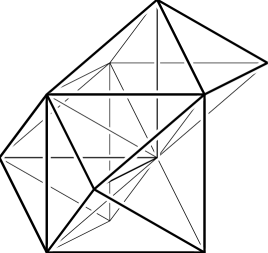
Figure 6: A possible unit cell of the dual to the tetrakaidekahedral lattice. There are many ways of constructing unit cells. This one is elementary and consists of twelve tetrahedra, which are – in groups of four – winding around the connections of the centre of the cube to the centres of the neighbouring cubes on top, in front, and to the left of this cube. None of the tetrahedral faces is part of a cubic face.

Its point-group symmetries are the same as the ones of the bcc lattice, i.e. $O_{h}$, and rotational symmetry of measurables is re-established for the Monte Carlo averages. The elementary unit cell of this lattice, together with it’s triangulation, is drawn in Fig. 7. We see that this lattice is interpretable as a simple cubic lattice subdivided as in type (b), and then tilted triclinically until rotational symmetry is restored. The necessary tilt turns the simple cubic lattice into a body–centred cubic one.

 

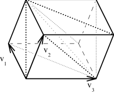
Figure 7: The elementary unit cell of the bcc lattice, with all the subdivisions to make it the dual of the tetrakaidekahedral lattice. The base vectors are $\vec{v_{1}}=\frac{1}{2}(-1,1,1)$, $\vec{v_{2}}=\frac{1}{2}(1,-1,1)$, and $\vec{v_{3}}=\frac{1}{2}(-1,-1,1)$

 

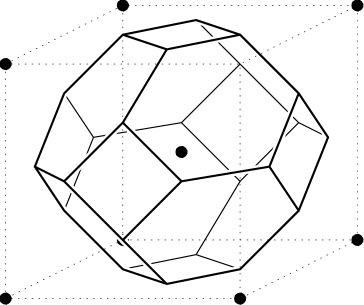
Figure 8: The first Brillouin zone of the bcc lattice, which is also the unit cell of the tetrakaidekahedral lattice. The field values are assigned to the centres of those cells (i.e. to the points of the bcc lattice), while the strings live on the edges.

Fig. 6 may be easier to interpret as far as lattice symmetries are concerned, but Fig. 7 is more supportive in the development of an efficient programming style.

As mentioned already, the unit cells of the dual lattice are almost spherical. This is desirable because the random phases assigned to lattice points live in the centres of the elementary unit cells of the dual lattice (or, more accurately, in the centre of the first Brillouin zone, which is only one representation of a minimal unit cell for the dual lattice). The unit cells of the dual lattice are therefore required to correspond to a correlation volume, which should obviously be close to spherical. The dual to our lattice is the tetrakaidekahedral lattice. The unit cell is essentially a cube with its vertices cut off half–way between the centre and the vertex of the cube (cf. Fig. 8).

To have a lattice which is both unique in its string configurations and rotationally symmetric in its predictions is an improvement to the VV method which we regard as highly necessary. Yet, another improvement has been made for the measurements in [15, 2]: the data structures corresponding to the string-data allow the lattice to be formally infinite.

4 The Self–Interacting Walk on an Infinite Lattice

Cosmic strings in the VV algorithm are a kind of locally self–interacting walk: There is no need to keep track of vacuum field values further away from the string than one correlation length. Effects from other strings are hidden in the randomly assigned vacuum field values. Every string can be traced from the information in the field values on the lattice sites. Unless a site has been visited by the same string already, we can just assign a random field value, and if a site is never visited by the string in question, we need not assign a field value at all.

In effect, we can ignore the whole lattice, and build up a corresponding data structure as we need it in the process of tracing the string. This data structure has to store the coordinates and assigned field values of only those lattice points which have been needed to tract the string. We then want a fast algorithm to check whether a particular lattice point has already needed an assignment of a random field value already during previous steps while tracing the same string, i.e. a fast way of checking whether given lattice coordinates are actually present in the data structure or not. If they are not, a random field value is assigned and the appropriate values are added to the walk data, otherwise the formerly assigned field value is re-used and nothing has to be added to the walk data (apart from whichever measurables one is interested in, of course; they are stored in a different data structure).

On a finite and storable lattice such a search algorithm is not needed because we can address each variable in the computer’s memory just by the lattice coordinates, without ever needing to worry whether there are any other pieces of (the same) string nearby.

Polymer physicists have studied the SAW, which is meant to describe configurational statistics of polymers in a low density solution [8, 34]. To trace out a SAW one has to check at every step whether the walk has already been at the lattice site which was randomly chosen to be the next one to be visited by the walk, and an efficient search algorithm is an essential ingredient for any method of tracing long walks  [21]. Naively one would expect the computational time for this to diverge as the square of the walk length (or even worse, since the possibility of running into a ‘dead end’ would have to be avoided at every step, which involves looking ahead an indefinite number of steps). However, much more sophisticated methods have become customary in that field [21], and the computational time spent on tracing the walk is usually just proportional to the walk length, i.e. the search time for nearby walk segments is of order one.

In the following sections we will introduce these methods into the VV type calculations, and argue that hash tables with collision resolution by double hashing [35] may be the most efficient data structure for such simulations.

4.1 A Simple Walk-Array

Seeing that the rest of the lattice can be ignored, one could store $L$ data elements in the computer’s memory, with $L$ being the total length of the walk. Every data element stores the coordinates of the lattice site which was needed to calculate the direction of the appropriate string segment together with the assigned field value. When making the next step in the walk, one looks through all the present array entries. The time it takes to search whether a given set of coordinates has occurred already in a walk of length $L$ is of order $L$. The total time it takes to trace such a walk is therefore proportional to $L^{2}$. Although the array will usually be much smaller than having $L$ elements (because of the high coordination number of our lattice a lattice site can be approached by the walk many times), this would be bad news if one wants to improve on the measurements made on finite lattices.

4.2 Classification of Coordinates: a List of Lists

As an improvement to this unstructured array, one can maintain separate lists for different subsets of the universe of coordinates. The set of coordinates is then used as a key from which we can compute which list we should search in. Of course one would like the given lists to be approximately equally populated in order to ensure that the algorithm does not effectively search in one long list most of the time, while leaving many short lists largely untouched. Apart from this the criterion by which to classify the universe of keys is entirely arbitrary. In [15] we used an algorithm of this kind, classifying the lattice points by their distance to the origin. The distance intervals were stacked such that they were expected to be equally strongly populated by walk elements. Since one does not know how far a given walk will distance itself from the origin, it is necessary to link the data lists dynamically, so that only as many lists as required for every particular walk are maintained. Every first element of the lists has therefore in addition to the pointer to the next element a pointer to the first element of the next list, which is only created when needed. A search for a given key involves then also a run through all the pointers of the first elements corresponding to all the distances shorter than the one of the key to the origin. A sketch of how the list of lists works is given in Fig. 9.

 

Figure 9: A possible layout of the list of lists after twelve coordinates have been stored, four of which happened to lie in the first distance interval from the origin, three lie in the second, and five in the third. For increased efficiency, the new elements should be stored on top of the lists, because they are more likely to be needed immediately again. More lists are added when the string moves into the fourth and higher distance intervals.

Keeping the length intervals too narrow slows down the search for the right list, whereas keeping them too wide slows down the search through the correct list. Therefore the width of these intervals has to be gauged to achieve a reasonable compromise. For well–tuned length intervals, one expects the average search time to diverge as the square root of the walk length. The time it takes to trace a walk then diverges proportionally to $L^{3/2}$. Note that the tuning procedure involves knowing the expected Hausdorff dimension of the walk, so that several runs may have to be done with probably non-uniform list lengths until the Hausdorff dimension is known.

4.3 Sorted Lists

A better technique has been used already in dynamical simulations of cosmic strings [19, 20]. There the lattice volume was divided into small boxes of dimensions comparable to the average string–string separation, and separate linked lists containing data for the string segments living within each of these boxes were maintained. This results initially in an array of lists, many of which could be empty. However, in the work for ref. [19], empty lists were eliminated from the array, and the remaining lists were sorted by a radix sort. If we were to use such a method for an infinitely large lattice in a VV simulation, the time it takes to search for the right list is of order $\log(m)$, where $m$ is the number of maintained (i.e. occupied) lists. It can easily be shown that search performance is optimised if $m\sim l$, i.e. if the average length of an occupied list is as small as possible. Every lattice site therefore gets its own box in the ideal adaptation of this algorithm to VV simulations. The average time of a search is then of order $\log(L)$, but an unsuccessful search, i.e. a search for lattice coordinates which have not yet been stored, has to be followed by an insertion of the new walk data somewhere in the array, taking a time of order $L$ to shift the subsequent array elements. This kind of insertion is not needed in the work of refs. [19, 20], because all searches are performed at time-slices of the string evolution, i.e. the whole array of lists is known from the beginning. While building up a self-interacting walk, the number of unsuccessful searches is proportional to $L$, thus the time to trace a string is dominated by those searches, and will be proportional to $L^{2}$.

It should be noted that the algorithm of [19, 20] works even without the elimination of empty lists from the array, because the lattices are finite. The sort algorithm is essential, however, for our gradually built-up lattice, such that the time-costly insertions cannot be eliminated.

4.4 Hash Tables

The proper adaptation of the algorithm in section 4.3, in spite of its other drawbacks for VV type simulations, eliminated entirely the $L$-dependence of the search time through the lists, by storing the data directly in the array without the use of lists (if we set $m=l$, i.e. the box size contains only one lattice point). How can the $L$-dependence of both the search for the right list and the time it takes to insert a new element be eliminated?

Let us see what the problem in section 4.2 was. The origin of the search-time associated with looking for the right list was that we didn’t know in advance how many lists would have to be maintained, i.e. how many classes of keys would be needed to describe the walk coordinates.

Let us now suppose we have a partition of the universe of keys into a fixed number of classes of keys. Then we can write the data into an array of lists, where the correct index is computed from the key and the appropriate list can be accessed directly without the use of pointers. The number of maintainable lists is then almost arbitrarily large (of order $L$ or larger), and search times through the lists become of order one. The prescription of how to compute the index – giving the position of the list in the array – from a given set of coordinates is called the hash function $h(x,y,z)$. Given that the set of coordinates one is likely to need is mapped onto the image of $h$ uniformly, the average search time needed to find a given set of coordinates which has been stored already is

$$\tau=1+\frac{n}{m}\,\,,$$

where $n$ is the number of lattice point which have already been stored, and $m$ is the number of linked lists ($n/m$ is the average length of a list, called the load factor $\alpha$ of the hash table). If the size of the array of lists is comparable to the walk length, then $\alpha$ is of order one and the average search time is also of order one.

Such an array of lists is called a hash table with collision resolution by chaining [35]. Collision resolution is the term for the method that tells us where to keep looking for the key (i.e. the set of coordinates of interest) if another key has been stored in the initially addressed data element. Chaining is the name for this method, if the place where we keep looking is a dynamically linked list.

4.5 Collision Resolution by Open Addressing

There is an even more efficient method for our purposes, which avoids the use of pointers altogether. It can only be used if no data entry has to be deleted until the whole hash table can be erased, but this is the case when one traces a static walk. In collision resolution by open addressing, every data element is stored in the original array, the hash table $T_{im}$, where $i$ is the index that counts the lattice coordinates and other variables to be stored for every point on the walk, and $m$ is of the order of, but larger than, the maximum length of any walk we would like to trace. First we compute the array index from the set of coordinates, using a hash function as the arbiter of the class partition of lattice points. If $U$ is the universe of keys – or the set or lattice sites – the hash function maps

$$h:\,U\rightarrow\{0,\ldots,m-1\}\,\,\,\,\,,\,\,\,\,\,$$ (6)

and appropriate variables for the key $k=(x,y,z)$, plus they key itself, will be stored in the slot $T_{i,h(k)}$ of the hash table $T$. Any $T_{i,}$ therefore contains $x,y,z$ and some set of variables $f(x,y,z)$. Obviously, collisions will occur for certain keys, i.e. $h(k_{1})=h(k_{2}),\mbox{~{}for~{}}k_{1}\neq k_{2}$. These can only be identified because the key itself has also been stored in the slots of $T$. To make collisions as unlikely as possible, one should make sure that all $h(k)$ are expected to be uniformly distributed over $\{0,\ldots,m-1\}$, and keep a low load factor $\alpha$. The time it takes to find a given set of coordinates in the hash table then depends on $\alpha$ and the method used for collision resolution. If we know that we can keep $\alpha<1$ and that we do not have to delete single elements from the hash table, collision resolution is best achieved by so-called open addressing, which gives us a rule by which to find an alternative slot in the hash table, if the slot we are searching in is already occupied by another key and its field data. Then we select a new $m$ which might still be empty, instead of appending a list of elements to the slot $T_{,m}$

4.6 Double Hashing

There are many ways of selecting alternative slots (cf. ref. [35]). The one we used in [2] is called double hashing: One uses two hash functions $h_{1},h_{2}:\,U\rightarrow\{0,\ldots,m-1\}$. The search algorithm looks first at the slot $T_{i,h_{1}(k)}$. If this slot is occupied by a different key from the one we are looking for, it looks at the slot with index $(\left[h_{1}(k)+h_{2}(k)\right]\bmod m)$, and so forth through all the $(\left[h_{1}(k)+nh_{2}(k)\right]\bmod m)$ for $n=0,\ldots,m-1$. If one encounters an empty slot before finding the key, then the key simply has not been used yet. A search in which the key is not found (since it has not been stored yet) is called an unsuccessful search. Insertion of new data is therefore preceded by an unsuccessful search, and the data is inserted at the first empty slot found. For collision resolution by double hashing the average time of an unsuccessful search is at most $1/(1-\alpha)$, while the average time of a successful search is at most $\frac{1}{\alpha}\left(1+\ln\left(1/(1-\alpha)\right)\right)$, but in any case less than the time for the average unsuccessful search (since it corresponds to an unsuccessful search at the time the given key was inserted, which was always at a time of a lower load factor), given that two restrictions on the choice of hash functions apply [35]:

• The set of $h_{1}(k),\,k\in U$ is uniformly distributed in $\{0,\ldots,m-1\}$.
  condition (1)

• $h_{2}(k)$ must be relatively prime to $m$ for all $k$, so that the whole hash table is searched if no empty slot can be found, i.e.
  $\{\left[h_{1}(k)+nh_{2}(k)\right]\bmod m\,|\,n\in\{0,\ldots,m-1\}\}\equiv\{0,\ldots,m-1\}$.
  condition (2)

Reasonable compromises between the desire for good memory utilisation and computational speed can be reached at load factors of about $1/2$ or $1/3$, although higher load factors are possible. One can gauge the desired compromise between efficient memory-utilisation and speed better than one can while using chaining for collision resolution, since the (essentially unknown) number or data collisions do not claim additional memory. Moreover, the absence of pointers reserves more memory for data in any case. Double hashing seems to be the most efficient method of open addressing. Others are linear and quadratic probing, which search the sequences $(h(k)+n){\rm mod}\,m,\,n=0,\ldots,m-1$ and $(h(k)+n+cn^{2}){\rm mod}\,m,\,n=0,\ldots,m-1$ respectively. For linear probing one gets clusters of occupied slots, which increase the probability of a further data collision, if one collision has occurred already in the search, and for quadratic probing it is generally quite difficult to ensure that all slots are searched through.

4.7 Example: Double Hashing on a bcc Lattice

It is now straightforward to apply hash tables with double hashing in VV-type algorithms. Remember that the assignment of field values happens randomly when the string comes into the vicinity of a lattice point for the first time, but that these values have to be recalled if the string approaches this point again at any later time. Using a hash table, we can simulate an arbitrarily large lattice, without considering more points than necessary. One can easily trace strings with lengths of up to $10^{7}$ lattice units on a small workstation without prohibitive memory requirements. This is a necessity for the accurate determination of the statistical measurables of e.g. the percolation model of string statistics in ref. [2].

It is particularly easy to create a uniformly distributed $h_{1}(k)$ on a simple cubic lattice ₃. For example, we could set $m$ to be of the form $m=s^{3}$, so that the set of all slots corresponds to the elements of ${}_{s}^{3}$, and cubes of edge-length $s$ can be stacked and mapped identically onto $\{0,1,\ldots,m-1\}$

$$h_{1}(x,y,z)=\left[x\bmod s+s(y\bmod s)+s^{2}(z\bmod s)\right]\,\,\,\,\,.\,\,\,\,\,$$ (7)

Condition (2) is fulfilled if $h_{2}(k)$ is relatively prime to $s$. This can be achieved by making $s$ a power of two, and ensuring that $h_{2}(k)$ is odd, for example

$$h_{2}(x,y,z)=\left\{2\left[y+sz+s^{2}x\right]+1\right\}\bmod m\,\,\,\,\,.\,\,\,\,\,$$ (8)

Note that $h_{2}(k)$ does not map every cube of size $s^{3}$ onto $\{0,\ldots,m-1\}$ in identical ways, so that coordinates that are identical modulo $s$ do have the same starting slot $T_{h_{1}}$, but a different search-sequence thereafter. Since $h_{2}$ has to be relatively prime to $m$, the uniformity of $h_{2}$ is somewhat restricted, but on average we still map onto all odd numbers $<m$ equally often.

Obviously, we cannot use Eq. 7 on the body-centred cubic lattice, since all the points have either only even or only odd coordinates, and $h_{1}$ would not be very uniform. We therefore create a unique map from the body-centred cubic lattice to a simple cubic one, and use as hash functions

$$g(x,y,z)=h\left(\left[\frac{x+1}{2}\right],\left[\frac{y+1}{2}\right],z\right)\,,$$ (9)

with $h$ being defined as $(h_{1}+nh_{2})\bmod m$, and $n$ the number of data collisions that had to be resolved to search for the desired slot in $T$. The Gauss bracket $\left[a\right]$ denotes the nearest integer not larger than $a$.

The hash functions Eqs. 7,8, and 9 are the ones used in ref. [2]. There, this algorithm allowed us to investigate a known percolation transition in string defect statistics [15] much closer than it is possible on a finite lattice. The transition was postulated in [16], but before the infinite lattice view it has been impossible to measure critical exponents of the transition appropriately. We found that the critical exponents of the percolation transition are in the same universality class as – and therefore identical with – standard bond or site percolation exponents. We were also able to measure the fractal dimension of string defects to higher accuracy, and to observe subtle differences between strings of only slightly different symmetry groups, while transforming $U(1)$ strings smoothly into $\R P^{2}$ strings.

Not specifying a lattice boundary also eliminates dramatic finite size errors, which are both very clearly observable [17] and well understood theoretically [36].

Conclusion

We have discussed necessary consistency requirements and improvements to the Vachaspati Vilenkin algorithm for Monte Carlo measurements of the statistics of cosmic strings and line disclinations.

We have shown a simple criterion which ensures that VV type simulations preserve the topological definition of the string flux through a given surface in the lattice description. We have suggested the use of a tetrahedral lattice to solve problems of uniqueness present on cubic lattices, although there are symmetry groups which escape a unique determination of the string shapes even on those lattices. We have argued that the lattice which is dual to the tetrakaidekahedral lattice combines further two desirable properties: it preserves the rotational symmetry of Monte Carlo averages, and it has only slightly varying edge lengths, making their correspondence to a well-defined physical correlation length more sensible. The first Brillouin zone of the dual lattice, which corresponds to a correlation volume after the string-forming phase transition, is close to spherical.

We have introduced the possibility to view string defects as locally self-interacting walks, allowing us to use a formally infinite lattice, which is built up as one needs it to construct the defects, and avoiding the specification of any boundary conditions.

This requires an efficient search algorithm to look up phase values on lattice sites lying on lattice plaquette which have been pierced by the string already. We find that a hash table algorithm with collision resolution by open addressing allows us to search for such points in a computational time of order one, permitting to trace a string in the time it takes to only write down the walk coordinates. Typically, a computer with 128MB of RAM will allow to trace strings of up to $10^{7}$ lattice units, which improves on measurements on finite lattices by two to three orders of magnitude.

References

- [1] T. Vachaspati and A. Vilenkin, Phys. Rev. D30 (1984) 2036.
- [2] K. Strobl and M. Hindmarsh, Sussex University preprint SUSX-TH-96-011 (hep-th/9608098).
- [3] T.W.B. Kibble, J. Phys. A 9 (1976) 1387.
-
[4]
I. Chuang, R. Dürrer, N. Turok and B. Yurke,
Science 251 (1991) 1336;
I. Chuang, B. Yurke, A.N. Pargelis and N. Turok, Phys. Rev. E47 (1993) 3343. - [5] M.J. Bowick, L. Chandar, E.A. Schiff and A.M. Srivastava, Science 264 (1994) 943.
- [6] P.C. Hendry, N.S. Lawson, R.A.M. Lee, P.V.E. MacClintock and C.D.H. Williams, Nature 368 (1994) 315.
- [7] W.H. Zurek, Los Alamos preprint LA-UR-95-2269 (cond-mat/9607135), to be published in Phys. Rep.
- [8] P.G. de Gennes, Scaling Concepts in Polymer Physics, (Cornell University Press, Ithaca, 1979).
- [9] S.F. Edwards and M. Warner, Phil. Mag. A40 (1979) 257.
- [10] N. Rivier and D.M. Duffy, J. Phys. C15 (1982) 2867.
- [11] R. Hagedorn, Nuovo Cim. Supp. 3 (1965) 147.
- [12] B. Sundborg, Nucl. Phys. B254 (1985) 583.
- [13] M.J. Bowick and L.C.R. Wijewardhana, Phys. Rev. Lett. 54 (1985) 2485.
- [14] D. Mitchell and N. Turok, Nucl. Phys. B294 (1987) 1138.
- [15] M. Hindmarsh and K. Strobl, Nucl. Phys. B437 (1995) 471.
- [16] T. Vachaspati, Phys. Rev. D44 (1991) 3723.
- [17] A.M. Allega, L.A. Fernández and A. Taranćon, Nucl. Phys. B344 (1990) 793;
- [18] T.W.B. Kibble, Phys. Lett. 166B (1986) 311.
- [19] E.P.S. Shellard and B. Allen, in “Formation and Evolution of Cosmic Strings”, eds. G. Gibbons, S. Hawking and T. Vachaspati (Cambridge University Press, Cambridge, 1990).
- [20] D. Bennett, ibid.
- [21] A.D. Sokal, in Monte Carlo and Molecular Dynamics Simulations in Polymer Science, Kurt Binder ed. (Oxford University Press, Oxford, 1994).
- [22] M.B. Hindmarsh and T.W.B. Kibble, Rep. Prog. Phys. 58 (1995) 477.
- [23] G.R. Vincent, M. Hindmarsh and M. Sakellariadou, Sussex University preprint SUSX-TH-96-008 (astro-ph/9606173).
- [24] N. Turok, in “Formation and Evolution of Cosmic Strings”, eds. G. Gibbons, S. Hawking and T. Vachaspati (Cambridge University Press, Cambridge, 1990).
- [25] S. Rudaz and A.M. Srivastava, Mod. Phys. Lett. A8 (1993) 1443.
- [26] M. Hindmarsh, A.–C. Davis and R. Brandenberger Phys. Rev. D49 (1994) 1944.
- [27] E.J. Copeland and P.M. Saffin, Sussex University preprint SUSX-TH-96-006 (hep-ph/9604231).
-
[28]
K. Strobl, Aspects of Approximate Symmetry in
Cosmology and Nematic Liquid Crystals (PhD thesis, Cambridge
University, 1995)
(http://starsky.pcss.maps.susx.ac.uk/users/karls/thesis/index.html). - [29] R.J. Scherrer and J.A. Frieman, Phys. Rev. D33 (1986) 3556.
- [30] E. Copeland, D. Haws, T.W.B. Kibble, D. Mitchell and N. Turok, Nucl. Phys. B298 (1988) 445.
- [31] R. Leese and T. Prokopec, Phys. Lett. B260 (1991) 27.
- [32] R.A. Leese and T. Prokopec, Phys. Rev. D44 (1991) 3749.
- [33] R.M. Bradley, P.N. Strensky, and J.-M. Debierre, Phys. Rev. A45 (1992) 8513.
- [34] B. Li, N. Madras and A.D. Sokal, New York Univ. preprint NYU–TH–94–09–01 (Sep. 1994).
- [35] T.H. Cormen, C.E. Leiserson and R.L. Rivest, Introduction to Algorithms (MIT Press/McGraw Hill, Cambridge MA/NY, 1990).
- [36] D. Austin, E. Copeland and R. Rivers, Phys. Rev. D49 (1994) 4089.