Study of Critical Slowing-Down in $SU(2)$ Landau Gauge Fixing

Abstract

We study the problem of critical slowing-down for gauge-fixing algorithms (Landau gauge) in $SU(2)$ lattice gauge theory on $2$ and $4$ dimensional lattices, both numerically and analytically. We consider five such algorithms, and we measure four different observables. A detailed discussion and analysis of the tuning of these algorithms is also presented.

1 INTRODUCTION

Here we report on the status of our study [1, 2] of Landau gauge-fixing algorithms. The efficiency of these algorithms is of key importance when gauge-dependent quantities — such as gluon and quark propagators — are evaluated, especially if the effect of Gribov copies is considered.

The main issue regarding the efficiency of these algorithms is the problem of critical slowing-down (CSD), which occurs when the relaxation time $\tau$ of an algorithm diverges as the lattice volume is increased (see for example [3]). Conventional local algorithms have dynamic critical exponent $z\approx 2$, namely $\tau\sim N^{2}$, while global methods may succeed in eliminating CSD completely, i.e. $z\approx 0$. We consider five different algorithms: the Los Alamos method (a conventional local algorithm), the Cornell method, which is generally believed to have $z\approx 2$, the overrelaxation and stochastic overrelaxation methods (improved local algorithms, which are expected to show $z\approx 1$), and the Fourier acceleration method, which is a global method. We confirm the predictions for $z$ (in both two and four dimensions) with the exception of the Cornell method. For this case we obtain that the dynamic critical exponent is actually $z\mathrel{\hbox to0.0pt{\lower 3.0pt\hbox{$\mathchar 536\relax$}\hss}\raise 2.0pt\hbox{$\mathchar 316\relax$}}1$, a result that can be understood by a comparative analysis between the Cornell and the overrelaxation methods. Besides the problem of CSD, we are also interested in understanding which quantities should be used to test the convergence of the gauge fixing, and in finding prescriptions for the tuning of parameters, when needed.

We consider the Standard Wilson action in $d$ dimensions:

$$S\left(\left\{U\right\}\right)\equiv\frac{4a^{d-4}}{g^{2}_{0}}\,\frac{1}{2}\sum_{\Box}(1\,-\frac{1}{2}\mathop{\rm tr}\nolimits U_{\Box})\;\mbox{.}$$ (1)

In order to fix the Landau gauge, we look for a local minimum of the function [4]

$${\cal E}\left(\left\{g\right\}\right)\;=\;1-\frac{a^{d}}{2\,d\,V}\sum_{\mbox{\boldmath$x$},\,\mu}\,\mathop{\rm tr}\nolimits U^{(g)}_{\mu}(\mbox{\boldmath$x$})$$ (2)

where

$$U_{\mu}^{\left(g\right)}(\mbox{\boldmath$x$})\;\equiv\;g(\mbox{\boldmath$x$})\;U_{\mu}(\mbox{\boldmath$x$})\;g^{\dagger}(\mbox{\boldmath$x$}+a\mbox{\boldmath$e$}_{\mu})\;\mbox{,}$$ (3)

and we start from $g(\mbox{\boldmath$x$})=1\!\!\!\bot$ for all $x$, keeping the thermalized configuration $\{U_{\mu}(\mbox{\boldmath$x$})\}$ fixed. [For the $SU(2)$ matrices we employ the usual parametrization $U\equiv u_{0}\,1\!\!\!\bot+i\,\vec{\mbox{$u$}}\cdot\vec{\mbox{$\sigma$}}$, where the components of $\vec{\mbox{$\sigma$}}$ are the three Pauli matrices.]

If $\{U_{\mu}^{\left(g\right)}\left(x\right)\}$ is a stationary point of ${\cal E}(\{g\})$ then we have the well-known result

$$\left[\left(\nabla\cdot A^{\left(g\right)}\right)(x)\right]_{j}=0\qquad\qquad\forall\;\;\;x\mbox{,}\;\;j\;\mbox{,}$$ (4)

namely the lattice divergence of each color component of the gauge field

$$A_{\mu}(\mbox{\boldmath$x$})\,\equiv\,\frac{1}{2ag_{0}}\left[\;U_{\mu}(\mbox{\boldmath$x$})-U_{\mu}^{\dagger}(\mbox{\boldmath$x$})\;\right]$$ (5)

is null. From equation (4) it follows that

$$Q_{\nu}(x_{\nu})\equiv\sum_{\mu\neq\nu}\sum_{x_{\mu}}A_{\nu}(\mbox{\boldmath$x$})$$ (6)

is constant, namely it is independent of $x_{\nu}$.

The algorithms we consider are all (with the exception of the Fourier acceleration) based on updating a single-site variable $g(\mbox{\boldmath$y$})$ at a time. As a function of $g(\mbox{\boldmath$y$})$ only, the minimizing function becomes

$${\widetilde{\cal E}}\left[g(\mbox{\boldmath$y$})\right]\,=\,constant\,-\,\frac{a^{d}}{2\,d\,V}\,\mathop{\rm tr}\nolimits[g(\mbox{\boldmath$y$})\,h(\mbox{\boldmath$y$})]\;,$$ (7)

where

$$h(\mbox{\boldmath$y$}) \equiv \sum_{\mu}\left[\;U_{\mu}(\mbox{\boldmath$y$})\;g^{\dagger}(\mbox{\boldmath$y$}+a\mbox{\boldmath$e$}_{\mu})\right.$$ (8)

$$\quad+\,\left.U_{\mu}^{\dagger}(\mbox{\boldmath$y$}-a\mbox{\boldmath$e$}_{\mu})\;g^{\dagger}(\mbox{\boldmath$y$}-a\mbox{\boldmath$e$}_{\mu})\;\right]$$

is the single-site effective magnetic field. Note that $h(\mbox{\boldmath$y$})$ is proportional to an $SU(2)$ matrix, i.e. we can write

$$h(\mbox{\boldmath$y$})\,\equiv\,{\cal N}(\mbox{\boldmath$y$})\,{\widetilde{h}}(\mbox{\boldmath$y$})\,\equiv\,\sqrt{\det h(\mbox{\boldmath$y$})}\,{\widetilde{h}}(\mbox{\boldmath$y$})\;\mbox{.}$$ (9)

We also define ${\cal T}(\mbox{\boldmath$y$})\,\equiv\,\mathop{\rm tr}\nolimits[\,g(\mbox{\boldmath$y$})\,{\widetilde{h}}(\mbox{\boldmath$y$})\,]$.

The single-site (multiplicative) update can be written as

$$g^{(new)}(\mbox{\boldmath$y$})\equiv R^{(update)}(\mbox{\boldmath$y$})\,g^{(old)}(\mbox{\boldmath$y$})\;\mbox{,}$$

and for the methods we consider we have (see [1] and references therein):

Los Alamos Method: in this case we have $g^{(new)}(\mbox{\boldmath$y$})\,=\,{\widetilde{h}}^{\dagger}(\mbox{\boldmath$y$})$, i.e. this update brings the single-site function ${\widetilde{\cal E}}\left[g(\mbox{\boldmath$y$})\right]$ to its unique absolute minimum;

Overrelaxation: here the matrix $R^{(update)}(\mbox{\boldmath$y$})$ is given by $[{\widetilde{h}}^{\dagger}(\mbox{\boldmath$y$})\,g^{\dagger}(\mbox{\boldmath$y$})]^{\omega}$, with $\omega\in(1,2)$; notice that the Los Alamos method corresponds to the case in which $\omega$ is equal to one, and that for $\omega=2$ the value of ${\widetilde{\cal E}}\left[g(\mbox{\boldmath$y$})\right]$ does not change;

Stochastic Overrelaxation: in this case the update $g^{(new)}(\mbox{\boldmath$y$})$ is given by

$$\left[{\widetilde{h}}^{\dagger}(\mbox{\boldmath$y$})\,g^{\dagger}(\mbox{\boldmath$y$})\,\right]^{2}\,g(\mbox{\boldmath$y$})\,=\,{\widetilde{h}}(\mbox{\boldmath$y$})\,{\cal T}(\mbox{\boldmath$y$})\,-\,g(\mbox{\boldmath$y$})\qquad\qquad$$

with probability $p$, and by ${\widetilde{h}}^{\dagger}(\mbox{\boldmath$y$})$ with probability $1-p\,$;

Cornell Method: here $R^{(update)}(\mbox{\boldmath$y$})$ is proportional to $\left[1\!\!\!\bot-\alpha\,a^{2}\,g_{0}\,\left(\nabla\cdot A^{\left(g\right)}\right)(\mbox{\boldmath$y$})\right]$; in [1] we prove that this can also be written as

$$\left[\,1\,-\,\frac{\alpha\,{\cal N}(\mbox{\boldmath$y$})\,{\cal T}(\mbox{\boldmath$y$})}{2}\,\right]\,1\!\!\!\bot\,+\,\alpha\,{\cal N}(\mbox{\boldmath$y$})\,{\widetilde{h}}^{\dagger}(\mbox{\boldmath$y$})\,g^{\dagger}(\mbox{\boldmath$y$})\;\mbox{;}\,\,\,\,\,\,$$

Fourier Acceleration: in this case the matrix $R^{(update)}(\mbox{\boldmath$y$})$ is proportional to

$$1\!\!\!\bot\,-\,\left\{{\widehat{F}}^{-1}\,\frac{p^{2}_{max}}{p^{2}(\mbox{\boldmath$k$})}\,{\widehat{F}}\left[\,\alpha\,a^{2}\,g_{0}\,\left(\nabla\cdot A^{\left(g\right)}\right)\right]\,\right\}(\mbox{\boldmath$y$})\;\mbox{,}$$

where ${\widehat{F}}$ is the Fourier transform, $p^{2}$ is defined as $(4/a^{2})\,\sum_{\mu}\,\sin^{2}\left(\,\pi\,a\,k_{\mu}\,\right)$, and $\,a\,k_{\mu}N$ takes the values $0\mbox{,}\,1\mbox{,}\,\ldots\mbox{,}\,N-1$. (Of course, to reduce the number of times the Fourier transform is evaluated, a checkerboard update should be employed.)

In order to determine the convergence of the gauge fixing, we measure the relaxation times $\tau_{i}$ for the following quantities [1]:

$${e_{1}}(t)\!\! \equiv \!\!{\cal E}(t-1)-{\cal E}(t)$$

$${e_{2}}(t)\!\! \equiv \!\!\frac{a^{d+4}\,g^{2}_{0}}{V}\sum_{\mbox{\boldmath$x$},\,j}\,\Big{[}\left(\nabla\cdot A\right)(\mbox{\boldmath$x$})\Big{]}_{j}^{2}$$

$${e_{4}}(t)\!\! \equiv \!\!\max_{\mbox{\boldmath$x$}}\left[\,1\,-\,\frac{1}{2}\,\mathop{\rm tr}\nolimits\,R^{(update)}(\mbox{\boldmath$x$})\right]$$

$${e_{6}}(t)\!\! \equiv \!\!\frac{1}{3d\,N}\,\sum_{\nu,\,j,\,x_{\nu}}\,\left[\,Q_{\nu}(x_{\nu})-{\widehat{Q}}_{\nu}\,\right]_{j}^{2}\left[{\widehat{Q}}_{\nu}\right]_{j}^{-2}$$

Here $t$ indicates the number of sweeps of the lattice and ${\widehat{Q}}_{\nu}\,\equiv\,1/N\,\sum_{x_{\nu}=1}^{N}\,Q_{\nu}(x_{\nu})$. We expect to observe that

$$e_{i}(t)\,\propto\,\exp\left(\,-\,t/\tau_{i}\,\right)\quad\mbox{with}\quad\tau_{i}=c_{i}N^{z_{i}}\;\mbox{,}$$ (10)

and also that all the quantities above have the same relaxation time $\tau$, and hence the same $c$, $z$.

2 RESULTS FOR $d=2$

For the four local methods we used [1] lattice sizes $N=8\mbox{,}\,12\mbox{,}\,\ldots\mbox{,}\,36$, while in the Fourier acceleration case we considered $N=8\mbox{,}\,16\mbox{,}\,32\mbox{,}\,64$. In all cases we have chosen the constant physics $N^{2}/\beta=32$, namely $N/\xi\approx 7$. We stopped the gauge fixing when the condition $e_{2}\leq 10^{-12}$ was satisfied.

From our data it is clear that the four quantities $e_{i}$ have the same $\tau$ for each given algorithm, as expected. However, for all the local updates — with the exception of the stochastic overrelaxation — the quantity $e_{6}$ was hardest to relax, namely its value was several orders of magnitude larger than the value of the other quantities. On the contrary, the Fourier acceleration method seems to be very efficient in relaxing $e_{6}$. Basing on these results, we think that the quantity $e_{6}$ allows a very sensible check of the gauge fixing and, in our opinion, it should always be used.

We evaluate the dynamic critical exponents $z$ from the weighted least-squares fit for $\tau=c\,N^{z}$, using lattice sizes $N\geq N_{min}\;$, and obtain [1]:

Los Alamos $$z=1.99\pm 0.04\;\mbox{,} \!N_{min}=12$$

Cornell $$z=0.83\pm 0.09\;\mbox{,} \!N_{min}=16$$

Overrelax. $$z=1.12\pm 0.07\;\mbox{,} \!N_{min}=16$$

Stoch. Overr. $$z=1.09\pm 0.05\;\mbox{,} \!N_{min}=12$$

Fourier $$z=0.04\pm 0.06\;\mbox{,} \!N_{min}=8$$

Clearly, the Fourier acceleration method is the most successful in reducing CSD, and it should be the method of choice when large lattice sizes are employed. However, the method is more costly per iteration than the local methods, and its CPU-time/site increases logarithmically with the lattice size. When this is taken into account, the total time for gauge fixing a configuration is smaller for Fourier acceleration than for the local methods if the lattice size is larger than about 300 sites, as can be seen in Figure 1. [Of course this result is very machine- and code-dependent. In any case, it seems unlikely [1] that the Fourier acceleration method would become the method of choice in two dimensions at lattice sizes $N$ smaller than around 100 sites.]

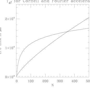
Figure 1: Comparison of the “effective” CPU-time/site ($T_{gf}$) between the Cornell method (the nearly straight line) and the Fourier acceleration.

3 TUNING

The need for tuning the parameters of an algorithm in order to get optimal efficiency is, of course, a potential disadvantage. Of the five algorithms we consider, all (but the Los Alamos method) require tuning. We did a careful analysis of this problem and we were able to verify a simple analytic expression for the optimal choice of $\omega$ (overrelaxation method), and to relate $\omega_{opt}$ to the optimal choice for the parameters of the other local methods. More specifically:

Overrelaxation: We tested the Ansatz [5]

$$\omega_{opt}\,=\,2\,\left[\,1\,+\,C_{opt}/N\,\right]^{-1}$$ (11)

and obtained very good agreement for lattice sizes greater than 12 with $C_{opt}=1.53\pm 0.35$. Note that, as the number of iterations $t$ increases, the matrix $R^{(update)}$ should approach the identity matrix $1\!\!\!\bot$. In this limit, the overrelaxation update can be written as [1]

$$g^{(over)}(\mbox{\boldmath$y$})\,\propto\,(1-\omega)\,g(\mbox{\boldmath$y$})\,+\,\omega\,{\widetilde{h}}^{\dagger}(\mbox{\boldmath$y$})\;.$$ (12)

Cornell Method: In this case, in the limit of large $t$, we can write [1]

$$g^{(Corn)}(\mbox{\boldmath$y$})\,\propto\,[1-\alpha\,{\cal N}(\mbox{\boldmath$y$})]\,g(\mbox{\boldmath$y$})\,+\,\alpha\,{\cal N}(\mbox{\boldmath$y$})\,{\widetilde{h}}^{\dagger}(\mbox{\boldmath$y$})\;\mbox{.}$$

By comparing this equation with (12), we made the conjecture $\alpha_{opt}\,\langle\,{\cal N}\,\rangle\,=\,\omega_{opt}$, with $\langle\,{\cal N}\,\rangle$ given by $2d\,(1\,-\,\langle\,{\cal E}_{min}\,\rangle)\;$. This Ansatz is very well fitted by our data [1].

Stochastic Overrelaxation: In this case it is not clear how to write a formula for the update as the number of iterations $t$ increases. A possibility [1] is to consider

$$g^{(stoc)}(\mbox{\boldmath$y$})\,\approx\,\left(\,1+p\right)\,{\widetilde{h}}^{\dagger}(\mbox{\boldmath$y$})\,-\,p\,g(\mbox{\boldmath$y$})\;\mbox{,}$$ (13)

which suggests the relation $p_{opt}\,=\,\omega_{opt}\,-\,1$. This conjecture seems to be satisfied reasonably well for lattice sizes larger than 30.

Fourier Acceleration: By analogy with the continuum $U(1)$ case, we expect [6]

$$a^{2}\,g_{0}\,(\nabla\cdot A^{\left(g\right)})(\mbox{\boldmath$y$})\propto\exp\left[-\alpha\,t\,a^{2}p^{2}_{max}\right]\;\mbox{,}$$ (14)

and therefore with the choice $\alpha_{opt}=(a\,p_{max})^{-2}\,$ we should obtain $\tau\propto{\cal O}(1)$. This gives, in $d=2$, a value ${\alpha_{opt}\,=\,0.125}$. This result is only in qualitative agreement with our data, which seem to indicate that $\alpha_{opt}\approx 0.16$ for large lattice sizes.

4 EXTENSION TO $d=4$

We study (in two and in four dimensions) the case $\beta=\infty$, namely we fix $U_{\mu}(\mbox{\boldmath$x$})=1\!\!\!\bot$ in (3) for all $x$ and $\mu$, and we look for a local minimum of the function (2) starting from a random configuration $\{g(\mbox{\boldmath$x$})\}$. In both the two and four dimensional cases, we essentially confirm the results obtained for $z$ at finite $\beta$ and in two dimensions [2].

It is interesting to notice that, in the case $\beta=\infty$, we can also write the minimizing function as

$${\cal E}\left(\left\{g\right\}\right)\,=\,\frac{a^{d}}{2\,d\,V}\sum_{\mbox{\boldmath$x$},\,\mu}\|\,g(\mbox{\boldmath$x$})\,-\,g(\mbox{\boldmath$x$}+a\mbox{\boldmath$e$}_{\mu})\,\|^{2}\mbox{.}$$ (15)

Here the $SU(2)$ matrix $g=g_{0}1\!\!\!\bot+i\,\vec{\mbox{$\sigma$}}\cdot\vec{\mbox{$g$}}$ is considered as a four-dimensional unit vector $(g_{0}\mbox{,}\,\vec{\mbox{$g$}})$ and $\|g\|^{2}\equiv g_{0}^{2}+\vec{\mbox{$g$}}\cdot\vec{\mbox{$g$}}$. When we are close to a minimum we can write

$$g(\mbox{\boldmath$x$})\,=\,1\!\!\!\bot-\,i\,\epsilon\,\vec{\mbox{$\sigma$}}\cdot\vec{\mbox{$f$}}(\mbox{\boldmath$x$})\,+\,{\cal O}(\epsilon^{2})\;\mbox{,}$$ (16)

where $\vec{\mbox{$f$}}(\mbox{\boldmath$x$})$ is a three-vector field. This gives

$$g(\mbox{\boldmath$x$})\,g^{\dagger}(\mbox{\boldmath$x$})\,=\,1\!\!\!\bot\,+\,{\cal O}(\epsilon^{2})$$ (17)

and

$${\cal E}\left(\left\{g\right\}\right)\,\approx\,\frac{\epsilon^{2}\,a^{d}}{2\,d\,V}\sum_{\mbox{\boldmath$x$},\,\mu}\|\,\vec{\mbox{$f$}}(\mbox{\boldmath$x$})\,-\,\vec{\mbox{$f$}}(\mbox{\boldmath$x$}+a\mbox{\boldmath$e$}_{\mu})\,\|^{2}\mbox{,}$$ (18)

namely (up to order $\epsilon^{2}$) we have the action of a three-vector massless free field $\vec{\mbox{$f$}}(\mbox{\boldmath$x$})$. Therefore we can use standard analytic methods [7] in order to study the problem of minimizing this quadratic form, and to compare the results for $z$, $\tau$ and the optimal choice of the parameters with our numerical data. Indeed, we find good agreement for all the quantities and methods considered [2].

Finally, we extend our simulations to the case $\beta=0$ (again in two and in four dimensions) [2]. All our results at $\beta>0$ are confirmed except for the Cornell method, for which we get $z\approx 2$, and for the Fourier method, which shows $z\approx 1$. In the Cornell case this result can be easily understood, since at $\beta=0$ its single-site update does not decrease the minimizing function at each step. In particular, the value of ${\cal E}$ increases if $\alpha{\cal N}(\mbox{\boldmath$y$})$ is large than two. [This is obvious if we consider the analogy between the Cornell method and the overrelaxation method, and the relation $\alpha{\cal N}(\mbox{\boldmath$y$})\sim\omega$. Moreover, it is plausible that only at very small values of $\beta$ we can have $\alpha\langle{\cal N}\rangle$ smaller than two and, at the same time, $\alpha{\cal N}(\mbox{\boldmath$y$})>2$ for a large set of lattice sites $y$.] However, we can recover the value $z\approx 1$ by redefining the Cornell single-site update in the following way [2]

$$g^{(Corn)}(\mbox{\boldmath$y$})\propto\left[1-\frac{\tilde{\alpha}(\mbox{\boldmath$y$}){\cal T}(\mbox{\boldmath$y$})}{2}\right]g(\mbox{\boldmath$y$})\,+\,\tilde{\alpha}(\mbox{\boldmath$y$})\,{\widetilde{h}}^{\dagger}(\mbox{\boldmath$y$})\,\mbox{,}$$

with $\tilde{\alpha}(\mbox{\boldmath$y$})\equiv\min\left(\,\alpha\,{\cal N}(\mbox{\boldmath$y$})\mbox{,}\;2\,\right)$. In the Fourier acceleration case we have the same problem: the update can increase the value of the minimizing function ${\cal E}$, and this happens most likely for small values of $\beta$. However, in this case we did not find a redefinition of the Fourier update [2] which could recover the value $z\approx 0$.

References

• [1] A.Β Cucchieri and T.Β Mendes, Nucl.Β Phys.Β B471 (1996) 263.
• [2] A.Β Cucchieri and T.Β Mendes, Critical Slowing-Down in Four-Dimensional $SU(2)$ Landau Gauge Fixing Algorithms, in preparation.
• [3] L.Β Adler, Nucl.Β Phys.Β  B (Proc.Β Suppl.) 9 (1989) 437; U.Β Wolff, Nucl.Β Phys.Β  B (Proc.Β Suppl.) 17 (1990) 93; A.Β D.Β Sokal, Nucl.Β Phys.Β  B (Proc.Β Suppl.) 20 (1991) 55.
• [4] K.Β G.Β Wilson, Recent Developments in Gauge Theories Proc.Β  NATO Advanced Study Institute (CargesΜ€e, 1979), eds.Β  G.Β  ’t Hooft et al.Β  (Plenum Press, New York–London, 1980).
• [5] J.Β E.Β Mandula and M.Β Ogilvie, Phys.Β Lett.Β  B248 (1990) 156.
• [6] C.Β T.Β H.Β Davies et al., Phys.Β Rev.Β D37 (1988) 1581.
• [7] H.Β Neuberger, Phys.Β Rev.Β Lett.Β  59 (1987) 1877; U.Β Wolff, Phys.Β Lett.Β  B288 (1992) 166.