DESY 96–151
HLRZ 96–55
HUB–EP–96/38
August 1996
Lattice computation of structure functions

Abstract

Recent lattice calculations of hadron structure functions are described.

1 INTRODUCTION

Since the late 1960’s, deep-inelastic scattering of unpolarised leptons and nucleons has been studied experimentally. The inclusive cross section for electroproduction can be described in terms of the structure functions $F_{1}$ and $F_{2}$ related to the densities of quarks and gluons in the nucleon (see, e.g., Ref. [1]). There is also some more indirect information on pion structure functions. Deep-inelastic scattering of longitudinally polarised leptons and nucleons allows one to measure two more structure functions, $g_{1}$ and $g_{2}$.

The observed scaling violations could be understood in the framework of perturbative QCD The computation of the structure functions themselves requires a nonperturbative method, e.g. lattice gauge theory and Monte Carlo simulations [2]. In this talk I shall describe recent attempts to calculate hadron structure functions on the lattice. An alternative method using the Hamiltonian version of lattice gauge theory is discussed in Ref. [3].

Instead of calculating the structure functions directly, we compute hadronic matrix elements of certain operators which, through the operator product expansion, are related to moments of the structure functions. In the deep-inelastic limit, the leading contribution is given by

$$2\int_{0}^{1}dx\,x^{n-1}F_{1}(x,Q^{2})=\sum_{f}c^{(f)}_{1,n}v^{(f)}_{n}(\mu)\,,$$ (1)

$$\int_{0}^{1}dx\,x^{n-2}F_{2}(x,Q^{2})=\sum_{f}c^{(f)}_{2,n}v^{(f)}_{n}(\mu)\,.$$ (2)

Here $n=2,4,6,\ldots$; $f$ labels the contributing operators, and $\mu$ is the renormalisation scale needed to define the (reduced) matrix elements $v^{(f)}_{n}$. The Wilson coefficients $c^{(f)}_{i,n}$ are calculated in perturbation theory and depend on $\mu^{2}/Q^{2}$ as well as on the coupling constant $g(\mu)$.

The operators we have to deal with are the “2-quark operators” (for $f=q=u,d$)

$${\cal O}^{(q)}_{\mu_{1}\cdots\mu_{n}}=\left(\frac{\mbox{i}}{2}\right)^{n-1}\bar{q}\gamma_{\mu_{1}}\mbox{ \parbox[b]{0.0pt}{$D$}\raisebox{7.3194pt}{$\leftrightarrow$}${}_{\!\mu_{2}}$}\cdots\mbox{ \parbox[b]{0.0pt}{$D$}\raisebox{7.3194pt}{$\leftrightarrow$}${}_{\!\mu_{n}}$}q$$ (3)

($D$ = covariant derivative) and (for $f=g$) purely gluonic operators, which contribute only in the flavour-singlet sector. For the nucleon the matrix elements $v^{(f)}_{n}$ are then defined by

$$\begin{array}[]{l}\displaystyle\mbox{\small$\frac{1}{2}$}\sum_{s}\langle p,s|{\cal O}^{(f)}_{\{\mu_{1}\cdots\mu_{n}\}}-\mbox{traces}|p,s\rangle\\ \displaystyle\quad{}=2v^{(f)}_{n}(p_{\mu_{1}}\cdots p_{\mu_{n}}-\mbox{traces})\,,\end{array}$$ (4)

where $|p,s\rangle$ denotes a nucleon state with momentum $p$ and spin vector $s$ ($s^{2}=-m^{2}$). Symmetrisation of all indices (indicated by $\{\cdots\}$) and subtraction of traces are needed to obtain operators transforming irreducibly under the Lorentz group, i.e. operators of definite twist = 2. Analogous results exist for pion and rho as well.

Within the parton model the $v^{(f)}_{n}$ are interpreted as average values of powers of the fraction of the hadron momentum carried by the parton (quark of flavour $q$ or gluon):

$$v^{(f)}_{n}=\langle x^{n-1}\rangle^{(f)}\,.$$ (5)

For the polarised nucleon structure functions one obtains in the chiral limit:

$$2\int_{0}^{1}dx\,x^{n}g_{1}(x,Q^{2})=\mbox{\small$\frac{1}{2}$}\sum_{f}e^{(f)}_{1,n}a^{(f)}_{n}(\mu)$$ (6)

for $n=0,2,4,\ldots$ and

$$\begin{array}[]{l}\displaystyle 2\int_{0}^{1}dx\,x^{n}g_{2}(x,Q^{2})\\ \displaystyle{}=\mbox{\small$\frac{1}{2}$}\frac{n}{n+1}\sum_{f}\left[e^{(f)}_{2,n}d^{(f)}_{n}(\mu)-e^{(f)}_{1,n}a^{(f)}_{n}(\mu)\right]\end{array}$$ (7)

for $n=2,4,\ldots$ with Wilson coefficients $e^{(f)}_{i,n}$ and reduced matrix elements defined by [4]

$$\begin{array}[]{l}\displaystyle\langle p,s|{\cal O}^{5(f)}_{\{\sigma\mu_{1}\cdots\mu_{n}\}}-\mbox{traces}|p,s\rangle\\ \displaystyle{}=\frac{a^{(f)}_{n}}{n+1}\left(s_{\sigma}p_{\mu_{1}}\cdots p_{\mu_{n}}+\cdots-\mbox{traces}\right)\,,\end{array}$$ (8)

$$\begin{array}[]{l}\displaystyle\langle p,s|{\cal O}^{5(f)}_{[\sigma\{\mu_{1}]\mu_{2}\cdots\mu_{n}\}}-\mbox{traces}|p,s\rangle\\ \displaystyle{}=\frac{d^{(f)}_{n}}{n+1}((s_{\sigma}p_{\mu_{1}}-s_{\mu_{1}}p_{\sigma})p_{\mu_{2}}\cdots p_{\mu_{n}}+\cdots\\ \displaystyle\hphantom{=}{}-\mbox{traces})\,.\end{array}$$ (9)

Here we need the operators (for $f=q$)

$${\cal O}^{5(q)}_{\sigma\mu_{1}\cdots\mu_{n}}=\left(\frac{\mbox{i}}{2}\right)^{n}\bar{q}\gamma_{\sigma}\gamma_{5}\mbox{ \parbox[b]{0.0pt}{$D$}\raisebox{7.3194pt}{$\leftrightarrow$}${}_{\!\mu_{1}}$}\cdots\mbox{ \parbox[b]{0.0pt}{$D$}\raisebox{7.3194pt}{$\leftrightarrow$}${}_{\!\mu_{n}}$}q\,.$$ (10)

Note that $d^{(f)}_{n}$ corresponds to twist 3. Within the parton model, $\mbox{\small$\frac{1}{2}$}a^{(q)}_{0}\equiv\Delta q$ is interpreted as the fraction of the nucleon spin carried by the quarks of flavour $q$.

Now the challenge for lattice QCD is the calculation of the reduced matrix elements $v_{n}$, $a_{n}$, $d_{n}$. So we have to compute forward hadron matrix elements of (relatively complicated) composite operators.

2 LATTICE CALCULATION

These matrix elements are calculated from three-point correlation functions. With suitable operators $B$, $\bar{B}$ for the particle to be studied, e.g. the nucleon, we can write schematically for $t>\tau>0$

$$\begin{array}[]{l}\displaystyle\langle B(t){\cal O}(\tau)\bar{B}(0)\rangle\\ \displaystyle{}=\langle 0|B\mbox{e}^{-H(t-\tau)}{\cal O}\mbox{e}^{-H\tau}\bar{B}|0\rangle\\ \displaystyle{}=\langle 0|B|N\rangle\mbox{e}^{-E_{N}t}\langle N|\bar{B}|0\rangle\langle N|{\cal O}|N\rangle+\cdots\end{array}$$ (11)

on a lattice with time extent $T\to\infty$. Correspondingly we have for the two-point function

$$\begin{array}[]{l}\displaystyle\langle B(t)\bar{B}(0)\rangle=\langle 0|B\mbox{e}^{-Ht}\bar{B}|0\rangle\\ \displaystyle{}\stackrel{{\scriptstyle t\to\infty}}{{=}}\langle 0|B|N\rangle\mbox{e}^{-E_{N}t}\langle N|\bar{B}|0\rangle+\cdots\end{array}$$ (12)

So we can determine the desired matrix elements from ratios of the form

$$R\equiv\frac{\langle B(t){\cal O}(\tau)\bar{B}(0)\rangle}{\langle B(t)\bar{B}(0)\rangle}=\langle N|{\cal O}|N\rangle+\cdots\,,$$ (13)

which should be independent of $\tau$ for $0\ll\tau\ll t$.

The bare lattice operators have of course to be renormalised and may mix with other operators in the process of renormalisation. In the euclidean continuum we should study operators like

$${\cal O}^{(q)}_{\mu_{1}\cdots\mu_{n}}=\bar{q}\gamma_{\mu_{1}}\mbox{ \parbox[b]{0.0pt}{$D$}\raisebox{7.3194pt}{$\leftrightarrow$}${}_{\!\mu_{2}}$}\cdots\mbox{ \parbox[b]{0.0pt}{$D$}\raisebox{7.3194pt}{$\leftrightarrow$}${}_{\!\mu_{n}}$}q\,,$$ (14)

$${\cal O}^{5(q)}_{\sigma\mu_{1}\cdots\mu_{n}}=\bar{q}\gamma_{\sigma}\gamma_{5}\mbox{ \parbox[b]{0.0pt}{$D$}\raisebox{7.3194pt}{$\leftrightarrow$}${}_{\!\mu_{1}}$}\cdots\mbox{ \parbox[b]{0.0pt}{$D$}\raisebox{7.3194pt}{$\leftrightarrow$}${}_{\!\mu_{n}}$}q$$ (15)

or rather O(4) irreducible multiplets with definite C-parity. In particular, we obtain twist-2 operators by symmetrising the indices and subtracting the traces. In the flavour-nonsinglet case they do not mix and are hence multiplicatively renormalisable.

Working with Wilson fermions (as we do) it is straightforward to write down lattice versions of the above operators. One simply replaces the continuum covariant derivative by its lattice analogue. However, O(4) being restricted to its finite subgroup H(4) (the hypercubic group) on the lattice, the constraints imposed by space-time symmetry are less stringent than in the continuum. In particular, a multiplet of operators which is irreducible with respect to O(4) will in general decompose into several irreducible H(4) multiplets and the possibilities for mixing increase [5, 6].

3 THE SIMULATIONS

Our simulations were performed on Quadrics parallel computers. We have worked on lattices of size $L^{3}\times T=16^{3}\times 32$ and $24^{3}\times 32$ at $\beta=6.0$ in the quenched approximation. For more technical details see Refs. [7, 8]. Most of our data were obtained with the Wilson action for the gauge fields and the quarks. First results from simulations with an improved fermionic action will however be discussed below (for more details see Ref. [9]).

The values of $\kappa$, $L$ and the (approximate) number of configurations used for the calculation of the nucleon matrix elements are the following :

$\kappa$		$L$	configs.
0.	1515	16	400
0.	153	16	600
0.	155	16	900
0.	155	24	100
0.	1558	24	100
0.	1563	24	100

Comparison of the $L=16$ and $L=24$ lattices at $\kappa=0.155$ will give us some information on finite size effects.

On the larger lattice we can use lighter quark masses without running into problems from severe finite size effects. This makes the extrapolation to the chiral limit more reliable, but the time needed to invert the fermion matrix increases considerably. So it becomes important that we choose our algorithm carefully. Therefore we have made a comparison between two popular choices, minimal residue with overrelaxation (MR) and a stabilised variant of the biconjugate gradient algorithm (BiCGstab).

Our main findings (for $\beta=6.0$, Wilson action quarks) are that if the quarks are not very light the MR algorithm, with an overrelaxation parameter $\omega=1.1$ was the most efficient algorithm, saving about 15 % in CPU time compared with BiCGstab. However as we approach $\kappa_{c}$ BiCGstab becomes the preferred algorithm. The $\kappa$ where the two inversion times cross over depends strongly on the lattice size. On a $12^{3}\times 16$ lattice the crossover is near $\kappa\approx 0.154$ while on the $24^{3}\times 32$ lattice BiCGstab does not become the better algorithm until $\kappa\approx 0.1555$. For our calculations we have therefore used the MR algorithm for the lower $\kappa$ values, the BiCGstab for the highest.

In order to suppress the unwanted excited states as much as possible it is important to choose the hadron operators judiciously. We do this by applying Jacobi smearing to the standard local operators. Both source and sink are smeared, since one needs a good projection on the ground state on both sides of the inserted operator in the three-point function. In the case of the proton we additionally use the “nonrelativistic projection” [7]. In this way we obtain a sufficiently long interval in $t$, where the two-point function is dominated by the ground state.

Our final choice of the operators whose matrix elements are calculated is motivated by the wish to avoid mixing (as far as possible) as well as momenta with more than one nonzero component. Taking the nucleon polarisation (where needed) in 2-direction and choosing the momenta $\vec{p}=(0,0,0),(2\pi/L,0,0)$ we studied the following operators and reduced matrix elements.

$v_{2,a}$	${\cal O}^{(q)}_{\{14\}}$
$v_{2,b}$	${\cal O}^{(q)}_{\{44\}}-\mbox{\small$\frac{1}{3}$}({\cal O}^{(q)}_{\{11\}}+{\cal O}^{(q)}_{\{22\}}+{\cal O}^{(q)}_{\{33\}})$
$v_{3}$	${\cal O}^{(q)}_{\{114\}}-\mbox{\small$\frac{1}{2}$}({\cal O}^{(q)}_{\{224\}}+{\cal O}^{(q)}_{\{334\}})$
$v_{4}$	${\cal O}^{(q)}_{\{1144\}}+{\cal O}^{(q)}_{\{2233\}}-{\cal O}^{(q)}_{\{1133\}}-{\cal O}^{(q)}_{\{2244\}}$
$a_{0}$	${\cal O}^{5(q)}_{2}$
$a_{2}$	${\cal O}^{5(q)}_{\{214\}}$
$d_{2}$	${\cal O}^{5(q)}_{[2\{1]4\}}$

The two operators for $v_{2}$ belong to different representations of H(4). Therefore their comparison gives an indication of the size of lattice artifacts.

Recently, first results have been obtained for nucleon matrix elements of operators of the type

$$\bar{q}\sigma_{\sigma\mu_{1}}\gamma_{5}\mbox{ \parbox[b]{0.0pt}{$D$}\raisebox{7.3194pt}{$\leftrightarrow$}${}_{\!\mu_{2}}$}\cdots\mbox{ \parbox[b]{0.0pt}{$D$}\raisebox{7.3194pt}{$\leftrightarrow$}${}_{\!\mu_{n}}$}q\,,$$ (16)

which are related to the so-called transversity distribution $h_{1}$ [10]. Purely gluonic operators have also been studied although they fluctuate much more than the 2-quark operators [11].

As explained above, we extract the hadronic matrix elements of our operators from the ratios $R$ (see (13)). In the case of the 2-quark operators we fix $t$, which allows us to compute the quark-line connected part of the three-point function for all values of $\tau$ and arbitrary operators ${\cal O}$ from quark propagators on two sources. The disconnected insertions, which would contribute in the flavour-singlet sector only, are however omitted. We choose $t$ as large as possible in order to have enough space for a “plateau” between 0 and $t$ where $R$ is independent of $\tau$. For the nucleon we took $t/a=13$ whereas in the case of the pion we adopted the symmetrical choice $t/a=16$ on our $16^{3}\times 32$ lattices.

Indeed we observe reasonable plateaus. Examples for the nucleon are shown in Ref. [7], an example for the pion is plotted in Fig.1. From the values of $R$ on the plateaus we can then calculate the reduced matrix elements taking into account kinematical factors, renormalisation constants etc. [7].

Figure 1: $R$ for the pion matrix element $v_{2,b}$ at $\kappa=0.153$ as a function of $\tau/a$.

Figure 2: $Z\times$Wilson coefficient for the matrix element $v_{2,a}$ at $\kappa=0.153$.

4 RENORMALISATION

Using 1-loop lattice perturbation theory we have calculated the matrix elements of all operators ${\cal O}^{(q)}_{\mu_{1}\cdots\mu_{n}}$ ($n\leq 4$) and ${\cal O}^{5(q)}_{\sigma\mu_{1}\cdots\mu_{n}}$ ($n\leq 2$) between quark states in the quenched approximation [12]. From these one can immediately compute the renormalisation constants and mixing coefficients for any linear combination that one wants to study. Increasing the accuracy of the required numerical integrations we obtained up to 8 significant digits. In the cases considered previously [6], our results agree with the older ones. In the following, we shall use the perturbative $Z$’s at the scale $\mu^{2}=a^{-2}\approx 5\mbox{GeV}^{2}$.

However, a nonperturbative determination is possible [13] and should eventually be preferred. In the end, the $\mu$ dependence of $Z$ must be cancelled by the $\mu$ dependence of the Wilson coefficient leading to renormalisation prescription independent results for the structure functions. In order to show to which extent this matching can be achieved we plot in Fig.2 the product of the nonperturbatively calculated $Z$ for $v_{2,a}$ with the corresponding renormalisation group improved nonsinglet Wilson coefficient versus $a^{2}\mu^{2}$. Indeed we obtain a reasonably flat region around $a^{2}\mu^{2}\approx 2$, though with a rather low value of $\Lambda_{\rm QCD}\approx 100{\rm MeV}$.

5 RESULTS FOR UNPOLARISED NUCLEON STRUCTURE FUNCTIONS

Plotting our results for $v_{2}$, $v_{3}$, $v_{4}$ versus $1/\kappa$ we can extrapolate (linearly) to the chiral limit. This is shown in Fig.3 for $v_{2}\equiv\langle x\rangle$ in the proton. (Similar pictures for $v_{3}$ and $v_{4}$ can be found in Ref. [7].) We see that the values obtained at smaller quark masses on the larger lattice ($24^{3}\times 32$) are consistent with those coming from the $16^{3}\times 32$ lattice. In particular, at $\kappa=0.155$ the numbers from both volumes agree within the errors. Furthermore we observe approximate consistency among $v_{2,a}$ and $v_{2,b}$ indicating the absence of large lattice artifacts (at least in this case).

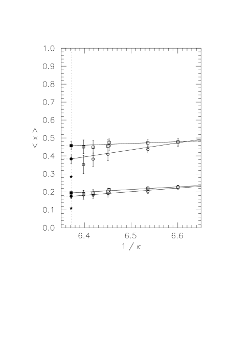
Figure 3: $\langle x\rangle$ for the proton (MOM scheme). The circles (boxes) correspond to $v_{2,a}$ ($v_{2,b}$). The upper (lower) band of data represents the results for the up (down)-quark distribution.

At this point it is impossible to resist the temptation to compare our results with experimental numbers. However, due to our use of the quenched approximation we can only compare with valence quark distributions. But even these will be influenced by the presence (or absence) of the sea. In fact, the phenomenological values indicated by the asterisks in Fig.3 differ substantially from the extrapolated lattice data. One might however expect that the flavour-nonsinglet combination $\langle x\rangle^{(u)}-\langle x\rangle^{(d)}$ is less sensitive to sea quark effects. Indeed our result of 0.23(3) ($\overline{\mbox{MS}}$ scheme) obtained by averaging $v_{2,a}$ and $v_{2,b}$ compares more favourably with the phenomenological number 0.18.

On the other hand, the large discrepancy between the quenched and the phenomenological values of $\langle x\rangle^{(q)}$ should not be too surprising. In the real proton the contributions of the valence quarks, the sea quarks, and the gluons must add up to 1. In the quenched approximation, the missing sea contribution, which is about 0.18, must somehow be compensated by the valence quarks and the gluons. Assuming that the gluon distribution is not too strongly affected by quenching one would expect the quenched $\langle x\rangle^{(q)}$ to be larger than the phenomenological result, which is exactly what we find.

The values obtained for $\langle x^{2}\rangle$ and $\langle x^{3}\rangle$ ($\overline{\mbox{MS}}$ scheme) differ less drastically from their phenomenological counterparts:

	lattice				experiment
	$u$		$d$		$u$		$d$
$\langle x\rangle_{a}$	0.	369(26)	0.	169(13)	0.	284	0.	102
$\langle x\rangle_{b}$	0.	440(22)	0.	187(10)	0.	284	0.	102
$\langle x^{2}\rangle$	0.	108(16)	0.	036(8)	0.	083	0.	025
$\langle x^{3}\rangle$	0.	020(10)	-0.	001(6)	0.	032	0.	008

6 RESULTS FOR POLARISED NUCLEON STRUCTURE FUNCTIONS

As in the case of the unpolarised structure functions, the chiral extrapolation of the $16^{3}\times 32$ data [7] is confirmed by the results obtained on the $24^{3}\times 32$ lattice at smaller quark masses. This is shown in Fig.4 for the case of $\Delta q$. In the chiral limit we find

$$\Delta u=0.84(5)\,,\,\Delta d=-0.24(1)\,.$$ (17)

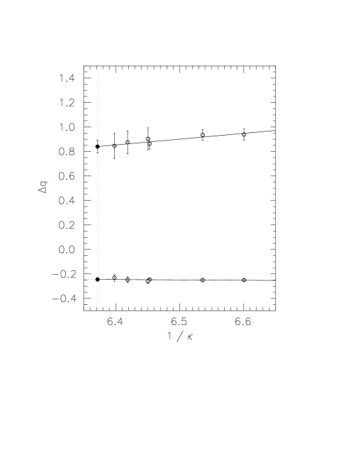
Figure 4: $\Delta u$ (upper values) and $\Delta d$ (lower values) for the proton.

These numbers should be compared with the fraction of the proton spin carried by the valence quarks (see, e.g., Ref. [14]):

$$\Delta u_{v}=0.92\,,\,\Delta d_{v}=-0.34\,.$$ (18)

Again one might hope that the difference of $u$ and $d$ contributions is less sensitive to quenching. One finds $\Delta u-\Delta d=1.08(6)$ to be compared with the axial vector coupling constant $g_{A}=1.26$.

In the higher moments of $g_{1}$ sea quark effects are also expected to be suppressed so that the quenched results should be reasonably close to the experimental numbers. For the proton we find

$$\int_{0}^{1}dx\,x^{2}g_{1}(x,Q^{2})=0.0150(32)\,,$$ (19)

where $Q^{2}=\mu^{2}\approx 5\mbox{GeV}^{2}$. The E143 collaboration obtains in a recent analysis 0.0121(10) [15].

7 PION STRUCTURE FUNCTIONS

In Fig.5 we summarise our results for the valence quark distribution in the pion obtained on a $16^{3}\times 32$ lattice [16]. We used the same operators as in the nucleon case. Like for $\langle x\rangle^{(u)}$ in the proton, $v_{2,b}$ is consistently larger than $v_{2,a}$. The three filled squares on the right represent the heavy quark limit, whereas those on the left are calculated from a phenomenological valence quark distribution [17].

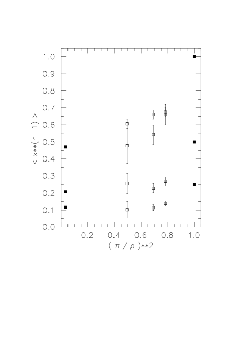
Figure 5: $v_{n}=\langle x^{n-1}\rangle$ for the pion versus $(m_{\pi}/m_{\rho})^{2}$ for $n=2,3,4$ (from top to bottom).

8 FIRST RESULTS FROM AN IMPROVED ACTION

Wilson’s fermion action suffers from $O(a)$ lattice artifacts. In order to suppress them at least in on-shell quantities, Sheikholeslami and Wohlert [18] added the so-called clover term

$$\frac{\mbox{i}}{4}c_{SW}a\sum_{x}\bar{q}(x)\sigma_{\mu\nu}F_{\mu\nu}(x)q(x)\,$$ (20)

to the action, where $F_{\mu\nu}$ is the clover-leaf lattice version of the field strength. For the coefficient $c_{SW}$ one obtains in lowest-order perturbation theory $c_{SW}=1$. A nonperturbative determination is however possible as the ALPHA collaboration has shown [19]. For $\beta=6.0$ they find the optimal value $c_{SW}=1.769$ [20], which should reduce the discretisation errors from $O(a)$ to $O(a^{2})$. Since a “canonical” value of $c_{SW}$ has not yet emerged, we have extended our perturbative calculation of renormalisation constants for the local 2-quark operators to the Sheikholeslami-Wohlert action with arbitrary $c_{SW}$ [21].

In order to improve matrix elements such as those considered here one needs in addition improved operators. We have obtained first results with perturbatively improved operators on a $16^{3}\times 32$ lattice at $\beta=6.0$ and $c_{SW}=1.769$ [9]. The value of $\Delta u-\Delta d$ in the chiral limit changes to 1.22(14) for $c_{SW}=1.769$ leading to better agreement with the experimental result 1.26.

9 CONCLUSIONS

This talk has described recent attempts to calculate hadron structure functions on the lattice. In the quenched approximation, at least the lower moments can be calculated with reasonable statistical accuracy.

Concerning the systematic uncertainties we can make the following statements:

• The comparison of results from $16^{3}\times 32$ and $24^{3}\times 32$ lattices does not reveal large finite size effects.

• The extrapolation to the chiral limit seems to be smooth. In the range of quark masses that we studied we did not observe any unexpected mass dependence with the possible exception of $d_{2}$.

• As a check for cut-off effects we calculated $\langle x\rangle$ from two different lattice operators. The outcome indicates that these effects are not too large. First results obtained with a nonperturbatively improved fermion action look promising.

Still there are further sources of systematic errors due to the renormalisation constants, the contributions of purely gluonic operators and fermion-line disconnected parts of 2-quark operators, etc. A major problem is, of course, the quenched approximation. However, the overall agreement with the real world is already rather satisfactory, at least as far as quantities are concerned which are expected to be less sensitive to quenching.

References

- [1] D. Soper, this conference.
- [2] G. Martinelli and C.T. Sachrajda, Nucl. Phys. B 306 (1988) 865; Nucl. Phys. B 316 (1989) 355. G. Martinelli, Nucl. Phys. B (Proc. Suppl.) 9 (1989) 134.
- [3] N. Scheu, this conference.
- [4] R.L. Jaffe, Comm. Nucl. Part. Phys. 19 (1990) 239.
- [5] M. Göckeler et al., preprint DESY 96-031, hep-lat/9602029.
- [6] G. Martinelli and Zhang Yi-Cheng, Phys. Lett. B 125 (1983) 77; S. Capitani and G.C. Rossi, Nucl. Phys. B 433 (1995) 351; G. Beccarini, M. Bianchi, S. Capitani and G.C. Rossi, Nucl. Phys. B 456 (1995) 271; S. Capitani, this conference.
- [7] M. Göckeler et al., Phys. Rev. D 53 (1996) 2317.
- [8] M. Göckeler et al., Nucl. Phys. B (Proc. Suppl.) 42 (1995) 337.
- [9] P. Stephenson, this conference.
- [10] S. Aoki, M. Doui and T. Hatsuda, preprint UTHEP-337, hep-lat/9606006; P. Rakow, this conference; A. Pochinsky, this conference.
- [11] R. Horsley, this conference.
- [12] M. Göckeler et al., preprint DESY 96-034, hep-lat/9603006.
- [13] G. Martinelli et al., Nucl. Phys. B 445 (1995) 81; M. Göckeler et al., Nucl. Phys. B (Proc. Suppl.) 47 (1996) 493; G.C. Rossi, this conference.
- [14] H.-Y. Cheng, H.H. Liu and C.-Y. Wu, preprint IP-ASTP-17-95, hep-ph/9509222.
- [15] K. Abe et al., Phys. Rev. Lett. 76 (1996) 587.
- [16] C. Best et al., in preparation.
- [17] P.J. Sutton, A.D. Martin, R.G. Roberts and W.J. Stirling, Phys. Rev. D 45 (1992) 2349.
- [18] B. Sheikholeslami and R. Wohlert, Nucl. Phys. B 259 (1985) 572.
- [19] K. Jansen et al., Phys. Lett. B 372 (1996) 275.
- [20] M. Lüscher and R. Sommer, private communication.
- [21] H. Perlt, this conference.