The Flat Phase of Fixed-Connectivity Membranes

Abstract

The statistical mechanics of flexible two-dimensional surfaces (membranes) appears in a wide variety of physical settings. In this talk we discuss the simplest case of fixed-connectivity surfaces. We first review the current theoretical understanding of the remarkable flat phase of such membranes. We then summarize the results of a recent large scale Monte Carlo simulation of the simplest conceivable discrete realization of this system [1]. We verify the existence of long-range order, determine the associated critical exponents of the flat phase and compare the results to the predictions of various theoretical models.

1 INTRODUCTION

Physical membranes, or 2-dimensional surfaces embedded in R³, are believed to have a high-temperature crumpled phase and a low temperature flat phase [2]. The flat phase is characterized by long range orientational order in the surface normals. Since long-range order is highly unusual in 2-dimensional systems, it is worthwhile developing a thorough understanding of this phase.

There are several experimental realizations of crystalline surfaces. Inorganic examples are thin sheets ($\leq 100$ Å) of graphite oxide (GO) in an aqueous suspension [3, 4] and the rag-like structures found in MoS₂ [5].

There are also remarkable biological examples of crystalline surfaces such as the spectrin skeleton of red blood cell membranes. This is a two-dimensional triangulated network of roughly 70,000 plaquettes. Actin oligomers form nodes and spectrin tetramers form links [6]. Crystalline surfaces can also be synthesized in the laboratory by polymerising amphiphillic mono- or bi-layers. For recent reviews see [7, 8, 9].

In this contribution we first review briefly the current analytical understanding of rigid membranes and then summarize the results of a recent large-scale Monte-Carlo simulation [1].

A Landau-Ginzburg-Wilson effective Hamiltonian for a $D$-dimensional elastic manifold with bending rigidity, embedded in $d$-dimensional space is

$$H_{\it eff} = \int{\rm d}^{D}\!\sigma\;\left[\frac{\kappa}{2}\left(\partial_{\alpha}\vec{\phi}_{\alpha}\right)^{2}+\frac{t}{2}\vec{\phi}_{\alpha}\cdot\vec{\phi}_{\alpha}\right.$$ (1)

$$+ \left.u\left(\vec{\phi}_{\alpha}\cdot\vec{\phi}_{\beta}\right)^{2}+v\left(\vec{\phi}_{\alpha}\cdot\vec{\phi}_{\alpha}\right)^{2}\right],$$

where the order field $\vec{\phi}_{\alpha}=\partial_{\alpha}\vec{r}$, and $\vec{r}(\sigma)$ is a vector in R^d. We are clearly dealing with a matrix $\phi^{4}$ theory. In the crumpled phase ($t>0$) the position vector $\vec{r}$ scales with system size $L$ like $\vec{r}\sim L^{\nu}$, with $\nu<1$, and hence $\phi_{\alpha}\sim L^{\nu-1}$. The exponent $\nu=2/d_{H}$ is the size or Flory exponent, where $d_{H}$ is the Hausdorff dimension. An expansion in $\phi_{\alpha}$ and its gradients is therefore justified. In the flat phase ($t<0$), the Hamiltonian is stabilized by the anharmonic terms. In mean field theory one finds that the induced metric $g_{\alpha\beta}$ has non-zero expectation value, $\langle\partial_{\alpha}\vec{r}\cdot\partial_{\beta}\vec{r}\rangle\propto\delta_{\alpha\beta}$.

The Hamiltonian Eq. (1) takes the following form in the flat phase

$$H_{\it eff}=\frac{1}{2}\int d^{D}\!\sigma\;\left[\left(\partial^{2}\vec{r}\right)^{2}+2\mu\,u_{\alpha\beta}^{2}+\lambda\,u_{\gamma\gamma}^{2}\right],$$ (2)

where the strain tensor $u_{\alpha\beta}=\frac{1}{2}(\partial_{\alpha}\vec{r}\cdot\partial_{\beta}\vec{r}-\delta_{\alpha\beta})$. The upper critical dimension for this model is 4 and it may be analyzed in a $\epsilon=4-D$ expansion. The most pressing physical question is the value of the lower critical dimension $D_{l}$. In particular one would like to know if $D_{l}\leq 2$, in which case physical membranes would indeed have a stable flat phase. The Hamiltonian Eq. (2) and the strain tensor $u_{\alpha\beta}$ can be re-written in the Monge gauge (see Figure 1) as

$$H_{\it eff}=\frac{1}{2}\int d^{D}\!\sigma\left[\kappa\,(\partial^{2}h)^{2}+2\mu\,u_{\alpha\beta}^{2}+\lambda\,u_{\gamma\gamma}^{2}\right]$$ (3)

and

$$u_{\alpha\beta}=\frac{1}{2}(\partial_{\alpha}u_{\beta}+\partial_{\beta}u_{\alpha}+\partial_{\alpha}h\partial_{\beta}h),$$ (4)

where $\mu$ and $\lambda$ are the Lamé coefficients.

Table 1: Theoretical predictions and numerical results.

	$\zeta$	$\eta_{u}$	$\nu={2}/{d_{H}}$	$\eta$
AL	${13}/{25}$ or 0.52	${2}/{25}$ or 0.08	1	${24}/{25}$ or 0.96
Large-$d$	${2}/{3}$	${2}/{3}$	1	${2}/{3}$
SCSA	0.590	0.358	1	0.821
MC	0.64(2)	0.50(1)	0.95(5)	0.62

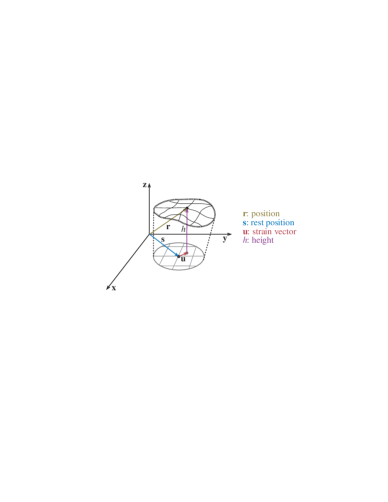
Figure 1: The Monge gauge.

By rescaling $\sigma\to s\sigma$, one sees that Eq. (3) in 4 dimensions is a function only of the dimensionless parameters

$$\tilde{\mu}=\frac{\mu}{\kappa^{2}}\;\;{\rm and}\;\;\tilde{\lambda}=\frac{\lambda}{\kappa^{2}}.$$ (5)

Aronovitz and Lubensky (AL) determined the RG flow of $\tilde{\mu}$ and $\tilde{\lambda}$ within the $\epsilon$-expansion, at fixed co-dimension, and found a globally attractive IR-stable fixed point at infinite bending rigidity [10]. This fixed point should control the properties of the whole flat phase [11, 12, 13]. In particular, we can introduce the anomalous scaling dimensions for the running coupling constants, $\kappa_{R}(q)\sim q^{-\eta}$ and $\mu_{R}(q)\sim\lambda_{R}(q)\sim q^{\eta_{u}}$. The generalization of Eq. (5) to $D$ dimensions relates the exponents $\eta$ and $\eta_{u}$ with the scaling identity

$$\eta_{u}=4-D-2\eta.$$ (6)

The roughness exponent $\zeta$, which governs the scaling of the height-height correlation function, is related to the exponent $\eta$ by the scaling relation $\zeta=(4-D-\eta)/2$. One may also study the Hamiltonian of Eq. (3) in a large-$d$ expansion in the non-linear sigma model limit (infinite Lamé coefficients) [14]. Finally one can solve a set of self-consistent equations (SCSA) for the scaling exponents of the renormalized coupling constants $\kappa$, $\mu$ and $\lambda$ [15]. The predictions for $\zeta$, $\eta$, $\eta_{u}$ and $\nu$ from the different approximations, and the results of our Monte Carlo (MC) simulations are summarized in Table 1.

2 THE MODEL

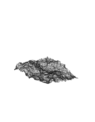
Figure 2: A snapshot of the surface in the flat phase for $L=46$.

In the simplest discretized version the crystalline surface is modeled by a regular triangular lattice with fixed connectivity, embedded in $d$-dimensional space. Typically the link-lengths of the lattice are allowed some limited fluctuations. This is usually modeled by tethers between hard spheres or by introducing some confining pair potential with short-range repulsion between nodes (monomers), such as Lennard-Jones. In some cases, the bending energy is explicitly introduced, and is represented by a ferromagnetic-like interaction between the normals to nearest-neighbor “plaquettes” [9].

We are interested in a much simpler model of a crystalline surface, inspired by the Polyakov action for strings [16]. The tethering potential between the particles is a simple Gaussian potential, with vanishing equilibrium length. Since the equilibrium length defines the bare elastic constants of the surface one may wonder whether such a model indeed exhibits the same phase diagram, and, in particular, if it has a stable flat phase.

$N$ particles are arranged in a regular triangular mesh. Each node in the interior has 6 neighbors. The action is composed of a tethering potential and a bending energy term:

$$H=\frac{1}{2}\sum_{\langle ij\rangle}(\vec{r}_{i}-\vec{r}_{j})^{2}+\frac{\kappa}{2}\sum_{\langle ab\rangle}(1-\vec{n}_{a}\cdot\vec{n}_{b})$$ (7)

where $\vec{r}$ is the position of node $i$, and $\vec{n}_{a}$ is the unit normal to face $a$. The sums extend to nearest neighbors. We point out that the normal-normal interaction translates to a next-to-nearest neighbor interaction (like a $\nabla^{2}$ term.) We do not include any minimum distance between the nodes. The model describes a phantom surface, since there is no self-avoidance term. While self-avoidance changes the nature of the crumpling transition, in the flat phase it is irrelevant (see Y. Kantor in [9].)

We choose to simulate a surface with free boundaries, since it simplifies the analysis of the correlation functions. The trade off is that we have to take careful account of edge fluctuations. This is described and illustrated in detail in [1].

3 OBSERVABLES

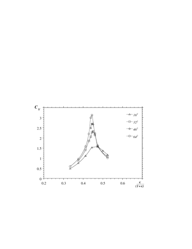
Figure 3: The specific heat $C_{V}$ versus $\kappa/(1+\kappa)$.

In order to estimate the exponents shown in Table 1 we measured several observables. For finite sizes, the specific heat $C_{V}$ peaks in the vicinity of a second order phase transition, or at coupling $\kappa\simeq\kappa_{c}$. The peak diverges with the exponent $\alpha\simeq 0.4$. We are currently increasing the statistics around the phase transition in order to determine $\alpha$ with greater accuracy. The main uncertainty affecting the estimate for $\alpha$ comes from the estimate of $\kappa_{c}$. We also measure $C_{V}$ in order to locate a region of the flat phase suitable for studying its scaling behavior. Note that, for a surface of finite size, the bending rigidity controls the importance of finite size effects. In order to obtain reliable finite size scaling one has to tune the correlation length $\xi\sim L$.

While $C_{V}$ indicates the location of the transition, it tells little about the nature of the phases on each side. Thus we measured the shape tensor and computed its eigenvalues. The shape tensor is the off-diagonal part of the inertia tensor $I_{\alpha\beta}$, being in some sense orthogonal to it. It is defined as

$$S_{\alpha\beta} = \left\langle\sum_{\sigma}r_{\alpha}(\sigma)r_{\beta}(\sigma)\right\rangle_{\!c}$$

$$= \delta_{\alpha\beta}\left\langle\sum_{\sigma}r_{\gamma}(\sigma)r_{\gamma}(\sigma)\right\rangle_{\!c}-I_{\alpha\beta},$$

where $\alpha$, $\beta$ refer to the components of $\vec{r}$, and the subscript $c$ indicates connected expectation values. The radius of gyration $R_{g}^{2}={\rm tr}S$ changes drastically across the transition. While for $\kappa<\kappa_{c}$ (hot phase) $R_{g}$ has small values compared with the linear size $L$ of the surface, for $\kappa>\kappa_{c}$ $R_{g}$ is large. More importantly the finite size scaling of $R_{g}\sim\L^{\nu}$ defines the size exponent $\nu=2/d_{H}$. In the crumpled phase $R_{g}\sim\log(L)$, and $\nu=0$. At the critical point $\nu$ has a non-trivial value. Above the critical point, in the flat phase, $\nu=1$ or $d_{H}=2$. Our measurement of $\nu=0.95(5)$ at $\kappa=1.1$.

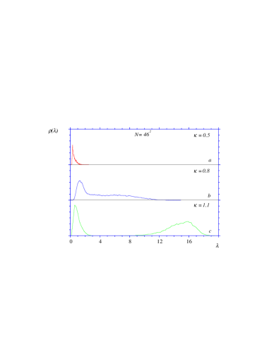
Figure 4: The distribution of eigenvalues of the shape tensor.

The eigenvectors of $S$ define a body-fixed frame on the surface; the eigenvalues of $S$ are the average square dispersions in the direction of the associated eigenvalue and tell more about the shape of the surface. Figure 4 shows the distribution of eigenvalues $\rho(\lambda)$ in the three regions of the phase diagram. Box a) shows $\rho$ in the crumpled phase: all three eigenvalues have identical distribution and the system is isotropic. Box b) shows $\rho$ in the vicinity of the transition: the system is still isotropic but the eigenvalues have fluctuations on large scales. Box c) shows $\rho$ in the flat phase: the surface is no longer isotropic — there is a well defined thickness and lateral extension, corresponding, respectively, to the left and right peak.

The roughness exponent $\zeta$ is measured from the finite size scaling of the average thickness of the surface. The minimum eigenvalue of $S$ provides just this information. This particular observable is very sensitive to boundary effects. In fact if an edge of the surface is “curled”, the eigenvalue will be considerably larger even if the surface is locally quite smooth.

In order to determine the influence of the boundary, we measured the average square thickness of several concentric hexagonal sub-sets of the surface of varying diameter $D$. We found that $\zeta$ plateaus in the range $L/4<D<3L/4$, shows boundary effects for $D>3L/4$ and discretization effects for $D<L/4$. We quote the value extracted from the plateau region (see Figure 5).

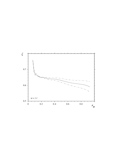
Figure 5: The roughness exponent $\zeta$ versus the diameter of the hexagonal sub-set of the surface.

The exponent $\eta_{u}$ can be extracted from the phonon fluctuations. It is in fact straight-forward to relate this observable and the exponent using the finite size scaling relation

$$\langle|\vec{u}|^{2}\rangle\sim L^{\eta_{u}}.$$ (9)

We have performed precise measurements of the phonon fluctuations, described in detail in ref. [1]. The determination of this exponent is important since it provides and independent consistency check of the scaling relation (6). Our measurement, shown in Table 1, is in good agreement with the theoretical predictions and the scaling relation.

Table 2: The number of thermalized sweeps collected per data point in the flat phase. The last column indicates the autocorrelation time for the slowest mode in the system, the radius of gyration.

$L$	$\kappa=1.1$	$\kappa=2.0$	$\tau_{R}\sim L^{z}$
32	$31\times 10^{6}$	$26\times 10^{6}$	$3\times 10^{4}$
46	$51\times 10^{6}$	$42\times 10^{6}$	$7\times 10^{4}$
64	$47\times 10^{6}$	$44\times 10^{6}$	$1.2\times 10^{5}$
128	$74\times 10^{6}$	—	$5\times 10^{5}$

Our final measurement of the properties of the flat phase of this model is the normal-normal correlation function. We expect the correlation function to fall off to a non-zero asymptote like

$$\langle\vec{n}_{\sigma}\cdot\vec{n}_{o}\rangle\;\sim\;C+\frac{c}{r^{\eta}},$$ (10)

where $r$ is the geodesic distance between the center $o$ and the point $\sigma$. Since the boundaries are free, the correlation function is not translationally invariant: we therefore fix the origin at the center of the surface and discard data too close to the boundary.

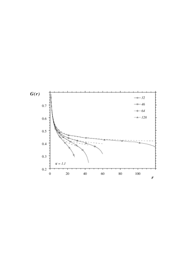
Figure 6: The normal-normal correlation function for different lattice sizes in the flat phase. The dashed lines are our best fit to Eq. 10.

In Figure 6 we show the behavior of the correlation function for different values of the lattice size. From the data in the figure it is clear that the normal-normal correlation function has a non-zero asymptote. The value of the asymptote grows with system size, and we believe it has a non zero infinite volume limit. The fit of the data to Eq. 10 gives yet another independent estimate of the exponent $\eta$. Our best fit to the $L=128$ data gives $\eta\simeq 0.62$, in good agreement with our previous estimates.

In conclusion, we have shown that the simple gaussian model of Eq. 7 faithfully reproduces the expected critical behavior of the AL fixed point. The relative simplicity of this model enables us to simulate surfaces of realistic size. The spectrin network of a blood cell has about 70,000 plaquettes; our largest surface has 32,768 plaquettes.

4 NUMERICAL METHODS

We will now turn our attention to the technical aspects of the simulation methods and the computers used. We use a Monte Carlo algorithm with a local Metropolis update. We choose a new position for a given node in a box of size $\epsilon^{3}$ centered on the old position, and we accept it according to the standard Metropolis test. A single Monte Carlo sweep consists of an update of all the nodes of the surface. The box size $\epsilon$ is adjusted so as to keep the acceptance ratio around 50%.

Table 3: Wall-clock timing results of the benchmark runs for different serial and parallel codes. The number are in seconds.

	Serial code	MPI code		HPF code
	A	A	B	A	B
Serial	334	—	—	4800	—
2	—	705	1410	2189	4378
4	—	400	1600	2375	9500
8	—	212	1696	—	—

Crystalline surfaces are characterized by extremely long autocorrelation times. The modes which suffer most are the ones related to the global shape of the surface in the embedding space. In table 2 we show the amount of data collected at various sizes/bending rigidities, and the corresponding autocorrelation time for the radius of gyration. We estimate the critical slowing down exponent $z$ to be $\simeq 2$, as expected for a local algorithm.

We are currently investigating several ways of improving the Monte Carlo simulations methods. In particular, we are studying different algorithms, like over-relaxation and uni/multi-grid Monte Carlo. Previous numerical studies have successfully taken the advantage of Fourier acceleration [17, 18, 19], and it is argued that multi-grid methods should perform similarly well [20, p. 41]. Preliminary tests of these algorithms give very encouraging results: over-relaxation reduces significantly the autocorrelation time, while we expect the multi-grid to improve the dynamical exponent $z$.

We used several workstations for most of the runs, but we simulated the largest lattice size ($L=128$) using a MASPAR MP1, a massively parallel processor, with exactly 16,384 nodes. Due to its hardware, the MP1 is best suited to run a Monte Carlo simulation with local update. Massively parallel processors are no longer common: workstation clusters with high speed switches are becoming more and more popular. This trend is reflected in the parallelization strategies that we are currently investigating.

While High Performance Fortran (HPF) is clearly the better choice for massively parallel computers, such as the MP1, it is still unclear whether its efficiency (or lack thereof) justifies its use in clustered environments. The alternative is to use the Message Passing Interface (MPI). This is a library of functions and a set of programming models which allows one to distribute a simulation over a cluster of workstations.

It is much simpler to write programs in HPF than MPI, since the HPF compiler automatically distributes the data on the various processors and it introduces the appropriate parallel instructions. The trade-off is that the programmer has little control over how the parallelization is actually done, and often the compiler does not exploit all of the potential parallelism of the algorithm. MPI allows much more flexibility and tailoring, but it is much harder to use since the parallelization must be coded by hand.

We have performed a series of benchmarks, using a simplified version of the code, in order to establish the efficiency of the different parallelization techniques. In Table 3 we compare the results of the benchmark runs. The first column shows the number of processors used in the run. This is an important factor: more processors mean more computing power, but also more message passing between the processors. While massively parallel computers had relatively low latency times for communication, clustered workstations often rely on a common switchboard with high latency times. The first column lists the elapsed time for a single processor run of the scalar code — this is the reference. The third and fourth column have the timings for the MPI code, written in c. Column A shows the elapsed time, while column B shows the integrated time (wall-clock time $\times$ number of processors). The fifth and sixth column show the timing of the HPF code. We note that, while for the MPI code the integrated time (column 3) grows slowly with the number of processors, for the HPF code (column 6) the time doubles, indicating very inefficient message passing. Based on our limited experience with our particular code, we believe that HPF is still far from being a viable choice for parallel programming on clustered environments.

Finally, we believe that farming (or running independent serial simulations on many processors) is still the most efficient solution for simulations small enough to fit on a single processor, since the integrated time for the MPI code is still higher than the single processor time.

5 ACKNOWLEDGMENTS

We would like to thank David Nelson, Mehran Kardar, Emmanuel Guitter, Alan Middleton, Paul Coddington, Enzo Marinari and Gerard Jungman for helpful discussions. NPAC (North-East Parallel Architecture Center) has provided the computational facilities. The research of MB and MF was supported by the Department of Energy U.S.A. under contract No. DE-FG02-85ER40237. SC and GT were supported by research funds from Syracuse University. Part of the work of KA was done at the Institute for Fundamental Theory at Gainesville and was supported by DOE grant No. DE-FG05-86ER-40272. We also acknowledge the use of the software package Geomview for membrane visualisation and code development [21].

References

- [1] M. J. Bowick et al., The flat phase of crystalline membranes, to appear in J. Phys. I (France).
- [2] D. Nelson and L. Peliti, J. Phys. France 48, 1085 (1987).
- [3] X. Wen et al., Nature 355, 426 (1992).
- [4] T. Hwa, E. Kokufuta, and T. Tanaka, Phys. Rev. A 44, R2235 (1991).
- [5] R. R. Chianelli, E. B. Prestridge, T. Pecoraro, and J. P. DeNeufville, Science 203, 1105 (1979).
- [6] C. F. Schmidt et al., Science 259, 952 (1993).
- [7] L. Peliti, in Fluctuating Geometries in Statistical Mechanics and Field Theory, edited by P. Ginsparg, F. David, and J. Zinn-Justin (cond-mat/9501076, Les Houches, France, 1994), lectures given at the Les Houches Summer School.
- [8] F. David, in Two Dimensional Quantum Gravity and Random Surfaces, Vol. 8 of Jerusalem Winter School for Theoretical Physics, edited by D. Gross, T. Piran, and S. Weinberg (World Scientific, Singapore, 1992).
- [9] Statistical Mechanics of Membranes and Surfaces, Vol. 5 of Jerusalem Winter School for Theoretical Physics, edited by D. Nelson, T. Piran, and S. Weinberg (World Scientific, Singapore, 1989).
- [10] J. Aronovitz and T. Lubensky, Phys. Rev. Lett. 60, 2634 (1988).
- [11] J. Aronovitz, L. Golubović, and T. Lubensky, J. Phys. France 50, 609 (1989).
- [12] E. Guitter, F. David, S. Leibler, and L. Peliti, Phys. Rev. Lett. 61, 2949 (1988).
- [13] E. Guitter, F. David, S. Leibler, and L. Peliti, J. Phys. France 50, 1787 (1989).
- [14] F. David and E. Guitter, Europhys. Lett. 5 (8), 709 (1988).
- [15] P. Le Doussal and L. Radzihovsky, Phys. Rev. Lett 69, 1209 (1992).
- [16] A. Polyakov, Nucl. Phys. B 268, 406 (1986).
- [17] M. Baig, D. Espriu, and A. Travesset, Nucl. Phys. B 426, 575 (1994).
- [18] D. Espriu and A. Travesset, Nucl. Phys. B (Proc. Suppl.) 47, 637 (1996).
- [19] J. Wheater, Nucl. Phys. B 458, 671 (1996).
- [20] A. D. Sokal, Monte Carlo mehtods in statistical mechanics: foundations and new algorithms, given at the Troisieme Cycle de la Physique en Suisse Romande, Lausanne, Switzerland, Jun 15-29, 1989.
- [21] M. Phillips, S. Levy, and T. Munzner, Notices of the American Mathematical Society 985 (1993), computers and mathematics column.