Simplicial Gravity In Dimension Greater Than Two

Abstract

We consider two issues in the DT model of quantum gravity. First, it is shown that the triangulation space for $D>3$ is dominated by triangulations containing a single singular $(D-3)$-simplex composed of vertices with divergent dual volumes. Second we study the ergodicity of current simulation algorithms. Results from runs conducted close to the phase transition of the four-dimensional theory are shown. We see no strong indications of ergodicity breaking in the simulation and our data support recent claims that the transition is most probably first order. Furthermore, we show that the critical properties of the system are determined by the dynamics of remnant singular vertices.

1 Quantum Gravity

The problem of reconciling the two theories of general relativity and quantum mechanics is perhaps one of the most important and difficult issues in theoretical physics. A variety of approaches have been adopted see eg.[1] but it is fair to say that only limited success has been achieved so far. In this article we shall concern ourselves with one such approach in which quantum mechanical fluctuations of the (Euclidean) geometry are encoded in a path integral.

$$Z\left(G\right)=\int{\cal D}[g]\exp{\left[-S\left(g,G\right)\right]}$$ (1)

We can take the action to be the standard Einstein-Hilbert term $S\left(g\right)=\frac{1}{16\pi G}\int d^{4}x\sqrt{g}\,R$ with gravitational coupling $G$. A variety of difficulties are immediately observed; firstly, $G$ carries dimensions of inverse mass squared so that the model is perturbatively nonrenormalizable. Perhaps worse $S$ is unbounded from below so it is not even clear that a stable vacuum exists. Furthermore, even when the functional integral is restricted to some fixed topology it is not clear that a unique choice exists for the functional measure ${\cal D}[g]$. The approach we have been following is to replace this continuum integral with a finite lattice sum in which these problems can be evaded or at least regulated. This approach is termed DT-gravity. Some of the excitement about this model has stemmed from the initial observations [2] that the four-dimensional theory appeared to exhibit a phase transition at finite bare $G_{0}$. This opened up the possibility of defining a continuum theory in the vicinity of this nonperturbative fixed point, perhaps in the spirit of Weinberg’s work on $2+\epsilon$ gravity [3].

2 Dynamical Triangulations

The basic idea is that one can divide $D$-dimensional space into a collection of equal volume elementary cells. The simplest choice for a cell is that it is a $D$-simplex — a set of $(D+1)$ fully interconnected points with edge length $a$ taken to be some invariant cut-off. A piecewise linear approximation to the manifold is then constructed by gluing these simplices together across their $(D-1)$-dimensional faces. Additional restrictions are also commonly employed in order to ensure that the neighborhood of any vertex is homeomorphic to a $D$-ball. The local scalar curvature density is then proportional to the number of simplices common to a given $(D-2)$-simplex which is bounded if the total volume is held fixed. Furthermore, its integral, the lattice action is essentially just the total number of nodes in the triangulation.

The partition function eqn 1 is then replaced by the lattice sum

$$Z=\sum_{T}\exp{\left[\kappa_{0}N_{0}-\kappa_{4}N_{4}-\left(\frac{\left(N_{4}-V\right)}{\Delta V}\right)^{2}\right]}$$ (2)

In practice the bare cosmological constant $\kappa_{4}$ is tuned to achieve a mean volume $\left<N_{4}\right>=V$ and the remaining coupling $\kappa_{0}$ plays the role of a bare Newton constant $G_{0}$. The parameter $\Delta V$ controls the size of the volume fluctuations.

There are many unknowns in this model. In this paper we consider just two — the structure of the measure over triangulations and the ergodicity of the simulation algorithms currently in use. As we shall see there are some intimate connections between these.

3 Singular Structures

Consider the triangulation space of the fixed volume $V$ ensemble for $D>3$. Let us define the local volume $\omega_{i}$ of some (sub)$i$-simplex as the number of simplices which contain that $i$-simplex. Let us also call this simplex singular if $\omega_{i}\to\infty$ as $V\to\infty$.

Our results can be summarized in two conjectures:

• Every triangulation contains exactly one singular $(D-3)$-simplex composed of $(D-2)$ singular vertices.

• The local volume $\omega\left(D-3\right)\sim aV^{\frac{2}{3}}$ while the singular vertex local volumes $\omega_{0}\sim bV$

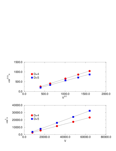
Figure 1: Singular local volumes for D=4,5

Fig 1 consists of two plots which illustrate these facts. The upper plot shows the volume of the singular $(D-3)$-simplex for $D=4,5$ against the two-thirds power of the total volume $V$. Clearly the data lies on a straight line verifying the first half of the second conjecture. The lower plot shows that the singular vertex volumes vary linearly with the total volume confirming the second part of this conjecture. Indeed, we have observed similar results in dimensions $D=6,7$ and can state that all the descendent subsimplices of the original singular $(D-3)$-simplex have local volumes which diverge linearly with the total volume in contrast to the sublinear growth observed for the $(D-3)$-simplex. Simple geometrical arguments are given in [4] for the two thirds power in the latter case. Indeed, the coefficient $a$ can also be predicted in terms of $b$ in this model and appears to fit the data rather well.

The immediate question that arises is why there are so many triangulations possessing this singular structure. It is simple to understand this by introducing the concept of a local entropy. Consider the set of simplices which form the local volume $\omega_{i}$ of some $i$-simplex and remove the common $(i+1)$ vertices. The remaining vertices and their interconnections then form a triangulation of a dual $(D-1-i)$ sphere. For example, a circle $S^{1}$ forms the boundary of the dual face to a link in three dimensions. The local entropy $s_{i}$ ascribed to that $i$-simplex is then defined to be equal to the number of ways of assembling the simplices in the local volume or equivalently the number of triangulations of this dual $(D-1-i)$-sphere.

$$s_{i}=Z_{D-1-i}\left(\omega_{i}\right)$$ (3)

This function is known to increase at least exponentially fast with volume for spheres with dimension greater than unity. Thus, $i$-simplices with $(D-1-i)\geq 2$ i.e. $i\leq(D-3)$ can increase their local entropy by growing their local volumes. It is then intuitively reasonable that a single singular $(D-3)$-simplex ultimately dominates composed of a cascade of smaller dimension secondary simplices.

Figure 2: Correlation of singular vertex volume with total vertex number close to the transition

This structure then forms a nonperturbative background in the crumpled phase of the model around which small fluctuations occur. Preliminary studies in four dimensions show that the volume of these singular vertices decreases monotonically as the coupling $\kappa_{0}$ increases. This is eminently reasonable since forcing more vertices into the system by increasing the coupling enhances the contribution of less singular triangulations (Singular ones have a minimal number of vertices for fixed volume).

Close to the phase transition a gas of remnant singular vertices exists whose fluctuations are highly correlated with the fluctuations of the total number of vertices. This is illustrated in fig 2 which shows a perfect (anti)correlation between the singular vertex volume $\omega_{0}$ and total vertex number $N_{0}$ for $V=32K$, $D=4$, $\Delta V=100$ and $\kappa_{0}=2.516$ (the pseudocritical coupling). Thus the peak in the node susceptibility is driven by the fluctuations in the singular simplex structure. The state with $\langle N_{0}\rangle\sim 6400$ has a large mean extent and essentially no singular vertices — a local volume of approximately 1000 means that the vertex has merged with the background distribution of vertex local volumes and can be no longer distinguished as a singular vertex. Correspondingly the state with $\langle N_{0}\rangle\sim 6200$ has a small extent and contains a variable number (at least one) of remnant singular vertices which are well separated from the background distribution. The critical system appears to tunnel repeatedly between these two states. We will return to this issue when we describe our experiments to check ergodicity.

4 Ergodicity

Current simulation algorithms typically target some volume $V$ and allow for some (usually rather small) fluctuations of size $\Delta V$ around this target value. It is known that for $\Delta V\to\infty$ the Monte Carlo algorithm used in the simulation is ergodic. That is all triangulations may be reached by the application of the elementary moves. However, the ergodic properties of the algorithm for finite $\Delta V$ are unknown. Indeed for $\Delta V<D$ the moves are known to be not ergodic. Thus it is important to check ergodicity carefully when studying the theory at finite $\Delta V$. In the light of recent claims that the four-dimensional theory has only a first order transition we have studied that model close to criticality, using large lattices and for three different values of the fluctuation volume $\Delta V=10,100,1000$. A dependence of expectation values on $\Delta V$ would signal a breaking of ergodicity. One way in which this could occur would be to suppose that the paths in the triangulation space between two volume $V$ triangulations required intermediate triangulations with much larger volumes. Barriers of height $B\left(V\right)$ might exist between states. Ergodicity would then be broken if

$$\Delta V\ll B(V)$$ (4)

Figure 3: Time series for $V=32K$, $\Delta V=1000$, $\kappa_{0}=2.516$

Fig 3 shows data for $V=32K$ and $\kappa_{0}=2.516\sim\kappa_{0}^{c}$ for $\Delta V=1000$. As for the earlier data presented in fig 2 the Monte Carlo time series clearly shows a sequence of tunneling events between two metastable states - this is the origin of the first order signal reported in [5]. Similar signals are seen at $\Delta V=10$ — we see no sign of a dependence of expectation values on $\Delta V$. Again, the two states can be labeled by a zero and non-zero number of remnant singular vertices.

Unfortunately, the situation is less clear for $V=64K$. A possible two-state signal is observed for $\Delta V=10,100$. The two states correspond to $\langle N_{0}\rangle\sim 12600$ and $\langle N_{0}\rangle\sim 13000$. However, since only one tunneling event is observed it cannot truthfully be distinguished from transient behavior associated with equilibration. Indeed, fig 4 shows the Monte Carlo time series for $\Delta V=1000$ and $\kappa_{0}=2.56\sim\kappa_{0}^{c}$ in which only the $\langle N_{0}\rangle=12600$ state is seen. After more than two million sweeps there is still no sign of a tunneling event to the other state. Clearly, it is difficult to use this large volume data to infer very much about the order of the transition due to the current lack of statistics.

Figure 4: Time series for $V=64K$, $\Delta V=1000$, $\kappa_{0}=2.56$

References

- [1] J. Ambjørn ”Quantization of Geometry”, Les Houches, Session LXII, 1994.
- [2] M. Agishtein and A. Migdal, Nucl. Phys. B385 (1992) 395; J. Ambjørn and J. Jurkiewicz, Phys. Lett. B278 (1992) 42; B. Brugmann and E. Marinari, Phys. Rev. Lett 70 (1993) 1908; S. Catterall, J. Kogut and R. Renken, Phys. Lett. B328 (1994) 277.
- [3] S. Weinberg, In ’General Relativity: an Einstein Centenary Survey’,ed. S.W. Hawking and W. Israel, Cambridge University Press 1979.
- [4] S. Catterall, G. Thorleifsson, J. Kogut and R. Renken, hep-lat/9512012, Nucl. Phys. B in press.
- [5] P. Bialas, Z. Burda, A. Krzywicki and B. Petersson, hep-lat/9601024; B. de. Bakker, hep-lat/9603024.