Correlations in fluctuating geometries

Abstract

We compare two definitions of connected correlation functions in fluctuating geometries. We show results of the MC simulations for 4D dynamical triangulation in the elongated phase and compare them with the exact calculations of correlation functions in the branched polymer model.

1 Introduction

Models of fluctuating(or random) geometries provide many challenging problems. One of them is the definition and interpretation of correlation functions. The usual formulation of the correlation function as a correlator of two observables in two fixed points at some distance apart is possible only if we have a fixed system of coordinates and a metric. This may be suitable for the perturbation thery approach. For theories like simplicial gravity, formulated in coordinate independent way, this is impossible. One way to proceed is to sum over all pairs of points with the fixed distance between them:

$$G^{OP}(r)=<\!\sum_{ij}v_{i}v_{j}O_{i}P_{j}\delta_{d(i,j),r}\!>.$$ (1)

The above average is taken over all geometries and the sum runs over all pairs of points at the fixed distance $d(i,j)=r$. The $v_{i}$’s denote some suitable volume elements. Next we define a “point-point” correlator:

$$<\!OP(r)\!>=\frac{G^{OP}(r)}{G^{11}(r)}$$ (2)

One immediate problem with those definitions is that these are not strictly speaking a two–point functions. The distance $d(i,j)$ depends on the geometry contrary to the usual fixed lattice case and it cannot be pulled out of the average. This leaves us with the average of a very non-local object.

2 Connected correlation functions

The next problem is the definition of the connected correlation functions. The straightforward standard substraction fails as was shown in [1]. The authors of [1] propose instead:

$$<\!OO(r)\!>_{c}^{*}=$$ (3)

$$\frac{1}{G^{11}(r)}<\!\sum_{ij}v_{i}v_{j}(O_{i}-<\!O(r)\!>)\cdot$$

$$\cdot(O_{j}-<\!O(r)\!>)\delta_{d(i,j),r}\!>$$

$$= <\!OO(r)\!>-<\!O(r)\!>^{2}$$

where

$$<\!O(r)\!>=\frac{G^{1O}(r)}{G^{11}(r)}$$ (4)

is the average of the observable $O$ over the spherical shells of radius $r$. This definition has nice properties, namely it vanishes with increasing $r$ as we would expect for a correlation fuction. But it does not integrate to a susceptibility. A definition which does integrate to a susceptibility was proposed in [2]:

$$<\!OO(r)\!>^{**}_{c}=$$ (5)

$$\frac{1}{G^{11}(r)}<\!\sum_{ij}v_{i}v_{j}(O_{i}-<\!O\!>)\cdot$$

$$\cdot(O_{j}-<\!O\!>)\delta_{d(i,j),r}\!>$$

$$= <\!OO(r)\!>-2<\!O\!><\!O(r)\!>+<\!O\!>^{2}$$

where $<\!O\!>$ is the usual average of $O$ over all the points of the lattice.

In the case of the fixed geometry $<\!O(r)\!>=\\ <\!O\!>$ and both definitions give indentical results. This is not so for fluctuating geometries. We plotted the two definitions with the observable being Regge curvature in simplicial 4D gravity in figure 1. They differ quite distinctly. The short distance behavior it totally different. For the large distances one can see that the definition (5) begins to deviate from zero, and as we will show later this is not due to errors but it is an intrinsic property of this function.

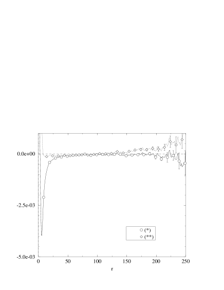
Figure 1: Correlation functions $<\!\!RR(r)\!\!>^{*}_{c}$ and $<\!\!RR(r)\!\!>^{**}_{c}$ in 4D simplicial gravity, $\kappa_{2}=1.5$, 32k simplices. For clarity only one in ten points is plotted.

2.1 Probabilistic interpretation

As to get some idea as to what causes those differences we can look at those function from the point of view of probability theory.

Let’s suppose that we make list of all pairs of points separated by the distance $r$ on all configurations. To each pair we assign a weight equal to the weight of the configuration times the volume elements of each point. We pick up a pair at random from this weighted list. The values of observable $O$ at each point of the pair will then define two random variables: $O_{1}$ and $O_{2}$. Then

$$<OO(r)>^{*}_{c}=E(O_{1}O_{2})-E(O_{1})E(O_{2})$$ (6)

where $E(O)$ denotes the expectation value of the operator $O$. The expression on the right hand side of this equation is zero if and only if the two variables are independent, so the definition (3) provides a direct measure of the degree of correlation between the values of observable $O$ in points at the distance $r$ apart.

To interpret the definition (5) we have to proceed a little differently. We make up a list of all points on all configurations. To every point we asign the weight of the configuration times its volume element. We pick up the random point $i$ from the list. We define now two random variables: $O_{i}$ the value of observable $O$ at the point and $S_{i}=\sum_{j}v_{j}\delta_{d(i,j),r}$ the volume of the spherical shell of radius $r$ around this point. Then

$$<\!O(r)\!>-<\!O\!>=$$ (7)

$$\frac{V}{G^{11}(r)}(E(OS)-E(O)E(S))$$

It easy to check that the square of the expresion on the left-hand side of the above equation is the difference between the definitions (3) and (5). So the definition (5) mixes in also the correlations between the value of an observable and the volume of spherical shell around it.

3 Branched polymers

To study these issues in more detail than permitted by todays status of the simplicial gravity simulations one can use other models of random geometry. One of such models is the branched polymer[3]. This model can be solved and correlation functions can be calculated for operators $q_{i}$ and $\log q_{i}$, where $q_{i}$ is the number of branches of vertex $i$ [4]. Interesting features of this particular model are that it describes the elongated phase of 4D simplicial gravity [5], and that it exibits a phase transition between a “short” and a “long” phase reminiscent of the transition in 4d simplicial gravity[6].

The results from this model for the function (3) are the following:
i) In the grand canonical ensemble this function is zero for positve values of $r$. This in a sense is a defining feature of the model: the branching probabilities are independent.
ii) In the canonical ensemble this function in the thermodynamical limit is power–like:

$$<\!\log(q)\log(q)(r)\!>^{*}_{c}\propto\frac{1}{(a+r)^{2}}$$ (8)

The correlations appear because the number of vertices is fixed. This is to be expected, but what is unusual is that those correlation persist even when the number of vertices grows to infinity. A possible mechanism could be the following: if we know that a vertex has one branch then its unique neighbour must have more than one branch, this introduces a correlation between nearest neighbour vertices which does not depend on the number of vertices. We believe that this effect is propagated to longer distances.
iii) Finite size effects alter this behaviour with the net effect of flattening the function at large $r$.

In figure 2 we have ploted the results of MC simulations in the elongated phase of 4d simplicial gravity. The effects described above are clearly visible: the functions are power like at short distances (with power exponent equal to 2.0 within errors) and then flatten due to the finite size with very good accord to the BP predictions.

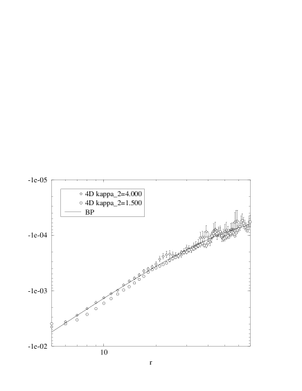
Figure 2: Correlation function $<\!\!RR(r)\!\!>_{c}^{*}$ for 4d simplicial gravity(32 k simplices) compared to the $<\!\!\log(q)\log(q)(r)\!\!>_{c}^{*}$ correlation function of branched polymers

For the definition (5) the results from BP are:
i) This function is not zero in the grand canonical ensemble. Althought the formula (7) is not valid in this ensemble a similar interpretation exists. This shows that this function contains also the correlations between the number of vertices at some distance from the point, and the number of branches of this point. Those are clearly dependent even in the grand canonical ensemble.
ii) In the canonical ensemble this definition is zero in thermodynamical limit ($r>0$). This implies a strong relation between branch-branch and branch-volume correlation, which is probably specific to the BP model.
iii) The convergence to the thermodynamical limit is not uniform. In particular the function will tend away from zero for $r\gg 1$ for any finite volume.

Figure 3: Correlation functions $<\!\!\log(q)\log(q)(r)\!\!>^{**}_{c}$ for branched polymers with two, four, eight and 16 thousand vertices. As the size of the polymer grows, the curves approach to zero.

These results are illustrated in the figure 3. It shows the $<\!\log(q)\log(q)(r)\!>^{**}_{c}$ correlation functions for branched polymers of various sizes. As the size increases the functions go to zero for any fixed $r$. However for each fixed size if we increase $r$ the functions will eventually go away from zero. We also see that this behavior agrees qualitatively with the results of MC simulations shown on figure 1.

4 Discussion

We have compared two definitions of connected correlation functions on the fluctuating geometries. Both were introduced in the context of simplicial gravity, each with a different goal in mind. To really compare and understand them we need a more profound understanding of the theory that we have now. One way to proceed is to study finite size scaling. This was the way proposed in [2]. The other way is to study the interaction of particles in the theory, this is in the spirit of [1, 7, 8]. It may happen that the functions describing the finite size scaling and the interaction potential are different. Both goals are still to be attained, and are quite difficult to pursue due to the enormous time required by simulations and very few theorethical results. That is why we propose the BP model as a very promising tool for gaining insight into these issues. As shown above this model provides an excellent description of the elongated phase of simplicial 4D gravity. In view of results from [6] it can hopefully also provide information about the critical region.

References

- [1] B. de Bakker, J. Smit, Nucl. Phys. B454 (1995) 343.
- [2] P. Bialas, Z. Burda, A. Krzywicki, B. Petersson Nucl. Phys. B472 (1996) 293.
- [3] J. Ambjørn, B. Durhuus, J. Fröhlich, P. Orland Nucl. Phys. B270 (1986) 457.
- [4] P. Bialas, Phys. Lett. B373 (1996) 289.
- [5] J. Ambjørn, J. Jurkiewicz, Nucl. Phys. B541 (1995) 643.
- [6] P. Bialas, Z. Burda Phase transition in fluctuating branched geometry hep-lat/9605020, to be published in Phys. Lett. B.
- [7] B. V. de Bakker, J. Smit “Gravitational binding in 4-d dynamical triangulation.” hep-lat/9604023.
- [8] J. Smit, this proceedings.