HU-TFT-96-32 The order of the phase transition in 3d U(1)+Higgs theory

Abstract

We study the order of the phase transition in the 3d U(1)+Higgs theory, which is the Ginzburg-Landau theory of superconductivity. We confirm that for small scalar self-coupling the transition is of first order. For large scalar self-coupling the transition ceases to be of first order, and a non-vanishing scalar mass suggests that the transition may even be of higher than second order.

1 Introduction

Scalar electrodynamics (i.e., the U(1)$+$Higgs theory) in three dimensions describes several different physical systems. First, it is an effective high-temperature theory for 4d scalar electrodynamics (with or without fermions) [1]. In particular, the 3d theory can be used to study the finite temperature phase transition in the 4d theory for small 4d coupling constants. Second, it is directly the Ginzburg-Landau theory of superconductivity. In this case, as well, the properties of the phase transition between the normal and superconducting states are of much interest [2, 3, 4, 5, 6, 7].

In general, the properties of the phase transition in the 3d U(1)+Higgs theory cannot be reliably studied in perturbation theory. This is due to the fact that the 3d coupling constants are dimensionful, resulting in infrared problems if there are nearly massless excitations (the true dimensionless expansion parameter is a coupling constant divided by a mass $\sim e_{3}^{2}/m_{H}(T)$). While the IR-problems are not quite as severe as in non-abelian theories containing gauge self-interactions, they nevertheless exist. In addition, non-perturbative topological defects play a role in U(1)$+$Higgs.

Due to the difficulties mentioned, the 3d U(1)$+$Higgs theory should be studied non-perturbatively [2, 3, 4, 5, 6, 7]. More specifically, some important problems to be addressed are: (a) the existence and order of a phase transition as a function of the scalar self-coupling, (b) the characteristics of the phase transition: the critical temperature $T_{c}$, latent heat, surface tension, correlation lengths in the two phases, and (c) the convergence of perturbation theory in the broken phase. We present here preliminary lattice results on (a); more complete results on (a) and (b) will be presented elsewhere [8]. (c) was addressed in [9].

2 The action and the parameters

The continuum U(1)$+$Higgs theory in 3d is defined by the action

$$S = \int d^{3}x\bigg{[}\frac{1}{4}F_{ij}F_{ij}+(D_{i}\phi)^{*}(D_{i}\phi)$$ (1)

$$+m_{3}^{2}\phi^{*}\phi+\lambda_{3}\left(\phi^{*}\phi\right)^{2}\bigg{]},$$

where $D_{i}=\partial_{i}+ie_{3}A_{i}$. The scale of the theory is given by the dimensionful [GeV] gauge coupling $e_{3}^{2}$, and the other two parameters are dimensionless,

$$x=\frac{\lambda_{3}}{e_{3}^{2}},\,\,\,y=\frac{m_{3}^{2}(e_{3}^{2})}{e_{3}^{4}}.$$

The parameter $x$ is roughly proportional to the ratio of the squares of the scalar and vector masses deep in the broken phase, $x\sim m_{H}^{2}/m_{W}^{2}$, while $y$ is related to temperature, $y\sim(T-T_{c})/T_{c}$. Here $T_{c}$ is the tree level critical temperature.

The Ginzburg-Landau theory of superconductivity is defined just by eq. (1). Conventionally, $m_{3}^{2},\lambda_{3}$ are denoted by $a,b$ in that context, and $x$ is represented by the Ginzburg parameter $\kappa=\sqrt{x}$. If $\kappa<1/\sqrt{2}$ the superconductor is of type I, if $\kappa>1/\sqrt{2}$ it is of type II. The phase transition is of first order for strongly type I superconductors, and for strongly type II superconductors it is usually assumed to be of second order.

3 Discretization and simulations

The action in eq. (1) can be discretized in the usual way. We use the compact formulation for the gauge field, so that the 3d lattice action is

$$S = \beta_{G}\sum_{P}{\mbox{Re}}\,(1-U_{P})$$ (2)

$$-\beta_{H}\sum_{x,i}{\mbox{Re}}\,\phi^{*}(x)U_{i}(x)\phi(x+\hat{i})$$

$$+\sum_{x}\phi^{*}\phi+\sum_{x}\beta_{R}\left[1-\phi^{*}(x)\phi(x)\right]^{2}.$$

Here $U_{i}(x)$ is the compact link variable, $U_{P}$ is the product of link variables around a plaquette $P$ and $\phi$ is a complex scalar field located on sites. It would also be possible to use a non-compact formulation [3, 4].

The three coupling constants in the lattice action are related to continuum parameters through a constant physics curve, which can be calculated using lattice perturbation theory. Due to the fact that the couplings are dimensionful, the relation can be found exactly with a 2-loop calculation [10]. The relevant relations are

$$\beta_{G}={1\over ae_{3}^{2}}, \beta_{R}={x\beta_{H}^{2}\over 4\beta_{G}},$$

$$2\beta_{G}^{2}\left({1\over\beta_{H}}-3-{2\beta_{R}\over\beta_{H}}\right) = y-(2+4x){\Sigma\beta_{G}\over 4\pi}$$

$$-{1\over 16\pi^{2}}\bigg{[}\left(-4+8x-8x^{2}\right)$$

$$\times\left(\ln 6\beta_{G}+0.09\right)+25.5+4.6x\bigg{]}.$$

The continuum limit is hence at $(\beta_{G},\beta_{H},\beta_{R})=(\infty,1/3,0)$. Note that increasing $\beta_{H}$ means decreasing $y$.

The simulations were done using Cray C94 at the Center for Scientific Computing in Helsinki.

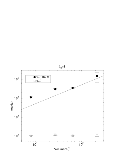
Figure 1: The maximum of the susceptibility $\chi$ as a function of volume. The straight line indicates the linear behaviour characteristic of first order transitions. The data point corresponding to the largest volume for $x=0.0463$ was obtained by reweighting the data.

4 The order of the transition

For small $x$, the phase transition in the 3d U(1)$+$Higgs theory is of the first order [2]. For larger $x$ (i.e., for type II superconductors), the IR-problems are more severe since the transition gets weaker, and the order has remained unclear. Arguments in favour of a second order transition have been given, e.g., in [3, 4, 5, 7], but a still higher-order transition cannot at present be excluded. In particular, in the lattice studies in [3, 4], the correlation lengths were not measured.

It is interesting to compare the situation with that in the 3d SU(2)$+$Higgs theory. There the line of first-order transitions ends at $x\sim 1/8$, and for $x>1/8$ the transition is of higher than second order [11]. An important difference between the U(1) and SU(2) cases is that in the latter all the excitations in the symmetric phase are massive, whereas in U(1) there should always be a massless photon in the continuum limit [6, 12, 13, 14]. Consequently, one can define an order parameter for the continuum theory [12]. Away from the continuum limit an exponentially small non-perturbative mass is generated in the compact lattice formulation [15], and the phases are analytically connected [16].

To study the order of the phase transition, we have used two different values of $x$. The first case $x=0.0463$ corresponds to a strongly type I superconductor, and the other case $x=2$ to a strongly type II superconductor.

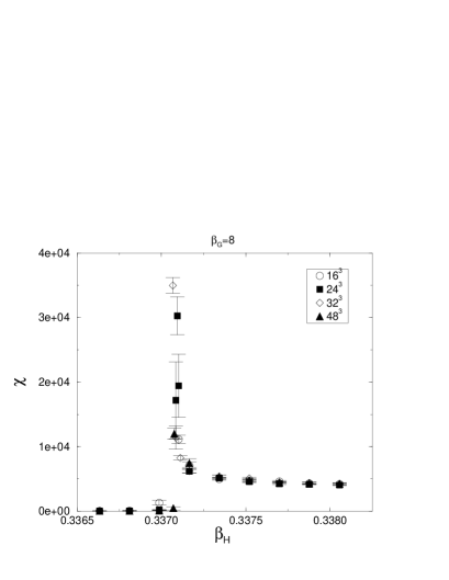
Figure 2: Susceptibility at $x=0.0463$.

In the analysis we follow closely [11]. The method employed is to plot the maximum of the susceptibility as a function of the lattice volume. The susceptibility $\chi$ is defined as

$$\chi=e_{3}^{2}V\left\langle(\phi^{*}\phi-\langle\phi^{*}\phi\rangle)^{2}\right\rangle.$$

In a first order transition $\chi$ grows as the volume $V$ and in a second order transition the expected behaviour is $\sim V^{\kappa}$, $\kappa$ being a critical exponent. If $\kappa\leq 0$, or if the transition is of higher than second order, $\chi\sim V^{0}$.

Figure 3: Susceptibility at $x=2$.

Our results are plotted in Fig. 1, and the individual susceptibilities in Figs. 2-3. The system has a first order phase transition at $x=0.0463$, as the maximum of susceptibility grows linearly with volume. This is not the case with the $x=2$ data, so the transition in strongly type II supercondutors is not of first order. The data would suggest that if the transition is of second order the critical exponent $\kappa$ is close to zero, as noticed already in [3, 4]. However, the transition might also be of higher order.

To study the transition at $x=2$ in more detail, we have measured the masses of the scalar and vector excitations. The masses are measured from the exponential decay of suitably chosen correlators. For the scalar mass we used the operator

$$\phi^{\ast}(x)\phi(x),$$

and for the vector mass

$$\mathop{\rm Im}\phi^{\ast}(x)U_{i}(x)\phi(x+\hat{i}).$$

The photon mass in the symmetric phase can be measured from the imaginary part of the plaquette variable at non-zero momenta [17].

The scalar mass is shown in Fig. 4 and the vector mass in Fig. 5. The scalar mass is clearly non-vanishing. For the vector mass the signal gets very noisy in the symmetric phase ($y>y_{c}$, $\beta_{H}<\beta_{H,c}$), and the techniques of [18] should be used. In general, improved techniques make the masses smaller so that, for example, the vector mass could go to zero at the phase transition point. Our very preliminary photon mass measurements in the symmetric phase are consistent with zero.

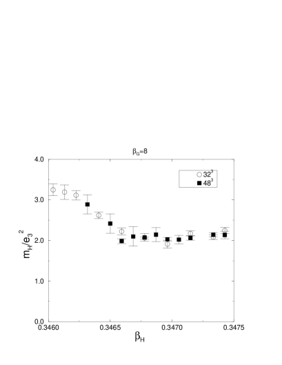
Figure 4: Scalar mass near the pseudocritical coupling $\beta_{H,c}$, for $x=2$. The values of $\beta_{H,c}$ can be seen from the maxima of $\chi$ in Fig. 3.

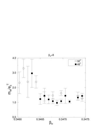
Figure 5: Vector mass near $\beta_{H,c}$ for $x=2$. Note that the high-temperature symmetric phase corresponds to $\beta_{H}<\beta_{H,c}$.

In conclusion, we have seen that in type II superconductors the phase transition is not of first order. It may even not be of second order, since we see a non-vanishing scalar mass. For definite conclusions we will have to improve the quality of mass measurements and study the finite $a$ effects.

References

- [1] P. Arnold, Phys. Rev. D 46 (1992) 2628; K. Farakos, K. Kajantie, K. Rummukainen and M. Shaposhnikov, Nucl. Phys. B 425 (1994) 67; A. Jakovác, A. Patkós and P. Petreczky, Phys. Lett. B 367 (1996) 283.
- [2] B.I. Halperin, T.C. Lubensky and S.-K. Ma, Phys. Rev. Lett. 32 (1974) 292.
- [3] C. Dasgupta and B.I. Halperin, Phys. Rev. Lett. 47 (1981) 1556.
- [4] J. Bartholomew, Phys. Rev. B 28 (1983) 5378.
- [5] J. March-Russell, Phys. Lett. B 296 (1992) 364.
- [6] W. Buchmüller and O. Philipsen, Phys. Lett. B 354 (1995) 403.
- [7] B. Bergerhoff, F. Freire, D.F. Litim, S. Lola and C. Wetterich, Phys. Rev. B 53 (1996) 5734.
- [8] K. Kajantie, M. Karjalainen, M. Laine and J. Peisa, in preparation.
- [9] M. Karjalainen and J. Peisa, HU-TFT-96-27 [hep-lat/9607023].
- [10] M. Laine, Nucl. Phys. B 451 (1995) 484.
- [11] K. Kajantie, M. Laine, K. Rummukainen and M. Shaposhnikov, CERN-TH/96-126 [hep-ph/9605288].
- [12] A. Kovner, B. Rosenstein and D. Eliezer, Nucl. Phys. B 350 (1991) 325.
- [13] A. Hebecker, Z. Phys. C 60 (1993) 271.
- [14] J.-P. Blaizot, E. Iancu and R.R. Parwani, Phys. Rev. D 52 (1995) 2543.
- [15] A.M. Polyakov, Phys. Lett. B 59 (1975) 82.
- [16] T. Banks and E. Rabinovici, Nucl. Phys. B 160 (1979) 349; E. Fradkin and S. Shenker, Phys. Rev. D 19 (1979) 3682.
- [17] B. Berg and C. Panagiotakopoulos, Phys. Rev. Lett. 52 (1984) 94; H.G. Evertz, K. Jansen, J. Jersák, C.B. Lang and T. Neuhaus, Nucl. Phys. B 285 (1987) 590.
- [18] O. Philipsen, M. Teper and H. Wittig, Nucl. Phys. B 469 (1996) 445.