The phase structure of the 3-d Thirring model

Abstract

We study the phase structure of the Thirring model in 3-d and find it to be compatible with the existence of a non gaussian fixed point of RG. A Finite Size Scaling argument is included in the equation of state in order to avoid the assumptions usually needed to extrapolate to the thermodymical limit.

1 Introduction

The Thirring model is a four-fermi theory with current-current interaction defined by the following continuum Lagrangian:

$${\cal L}=\bar{\psi}_{i}(\partial{\!\!\!/}\,+m)\psi_{i}+{g^{2}\over{2N_{f}}}(\bar{\psi}_{i}\gamma_{\mu}\psi_{i})^{2}$$ (1)

where $\psi$ and $\bar{\psi}$ are four-fomponent spinors, $m$ is a bare mass, and $i$ runs over $N_{f}$ fermion species.

As in the case of the Gross-Neveu model (GN), naïve power counting suggests that the theory is not renormalizable in the usual perturbative expansion in powers of the coupling constant. Nonetheless, different approaches might allow a continuum limit to be defined for these theories. It has been established, using the $1/N_{f}$ expansion, that GN is renormalizable to all orders, showing an interesting phase structure with an UV fixed point of RG, spontaneous chiral symmetry breaking with dynamical mass generation and a spectrum of mesonic bound states.

For the Thirring model the situation is less clear. The $1/N_{f}$ expansion turns out to be renormalizable (at least at leading order), but neither chiral symmetry breaking nor charge renormalization are observed (the $\beta$-function vanishes identically for all values of the bare coupling). On the other hand chiral symmetry breaking and dynamical mass generation are expected at some critical value of the coupling $g_{c}(N_{f})$, from the solution of Schwinger-Dyson equations. However, in order to solve these equations, one has to use some Ansatz for the 1-PI vertex function. According to the chosen Ansatz, the functional dependence of $g_{c}$ on $N_{f}$ turns out to be different. This inconsistent picture can be clarified by a lattice study of the model.

The existence of a non-gaussian fixed point, allowing a strongly interacting theory with dynamical mass generation to be defined, would be of great theoretical interest. It has a phenomenological relevance for model-building beyond the Standard Model and it can describe high-$T_{c}$ superconductivity and the IR behaviour of $QED_{3}$. Besides, due to its relative simplicity, the 3-d model is an ideal laboratory to compare different non-perturbative approaches and to test algorithms for simulating dynamical fermions.

2 Lattice formulation

We simulate the theory using $N$ species of staggered fermions and a non-compact action:

$$S = \frac{1}{2}\sum\bar{\chi}_{i}(x)\eta_{\mu}(x)\left[1+iA_{\mu}(x)\right]\chi_{i}(x+\mu)$$ (2)

$$+ \mbox{h.c.}+m\sum\bar{\chi}_{i}\chi_{i}+\frac{N}{4g^{2}}\sum A^{2}_{\mu}$$

For $N=1$ this is equivalent to the compact formulation where the interaction term becomes $\bar{\chi}(x)\exp(iA_{\mu}(x))\chi(x+\mu)$ and the mass term for the vector field is no longer needed. Both lattice formulations have their drawbacks. For $N>1$, the compact version generates higher order interactions (six fermions vertices) when the auxiliary field is integrated out. The non-compact one has an additive charge renormalization, preventing to perform numerical simulations at arbitrary strong coupling (see [1] for details).

3 Data analysis: the Equation of State

The data are obtained, as usual, from numerical simulations at finite values of the bare mass and on finite lattices. In order to study dynamical mass generation, we need to consider the $m\rightarrow 0$ limit, while we also have to take into account the relevance of finite size effects. The only assumption we are going to make in analyzing our data is that the RG flow for the Thirring model is similar to the one observed for GN: we therefore expect to have a critical coupling $g_{c}(N)$, corresponding to an UV fixed point, where a chiral symmetry breaking phase transition occurs, separating a massless phase at weak coupling from a massive one at strong coupling. Being below the upper critical dimensions ($d=4$), one can solve the RGE without worrying about logarithmic corrections to scaling.

An equation of state can then be derived using the solution of the RG equations for the external magnetic field at given magnetization [2]. In our case, the external, symmetry-breaking field, is the bare mass $m$, and the magnetization is the order parameter monitoring the symmetry breaking, i.e. the chiral condensate. In terms of the scaled variables, we obtain:

$$m\langle\bar{\psi}\psi\rangle^{-\delta}={\cal F}_{1}\left(t\langle\bar{\psi}\psi\rangle^{-1/\beta}\right)$$ (3)

where $t=1/g^{2}-1/g_{c}^{2}$ and ${\cal F}_{1}$ is a universal scaling function.

In order to take into account finite size effects, we introduce the volume of the lattice as a scaling field of dimension $d$. The scaling function depends now on two independent combinations of rescaled variables:

$$m\langle\bar{\psi}\psi\rangle^{-\delta}={\cal F}_{2}\left(t\langle\bar{\psi}\psi\rangle^{-1/\beta},L^{-1/\nu}\langle\bar{\psi}\psi\rangle^{-1/\beta}\right)$$ (4)

where $L$ is the linear size of the lattice.

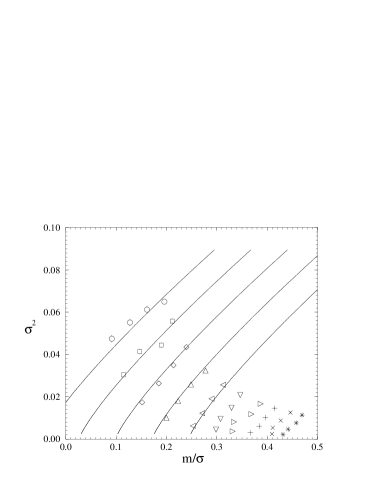
Figure 1: Fisher plot for $N=1$, from data at $\beta=1.6(\triangle)$, $1.8(\triangleleft)$, $2.0(\nabla)$, $2.2(\triangleright)$, $2.4(+)$, $2.6(\times)$, on a $12^{3}$ lattice.

In the limits $L\rightarrow\infty$, $t=0$ or $m=0$, Eq. (4) reproduces the usual definitions of the critical exponents $\nu$, $\delta$ and $\beta$. Neglecting the finite-size correction and performing a Taylor expansion of ${\cal F}_{1}$ for small $t$, one obtains a five parameter equation to which the lattice data at fixed lattice volume can be fitted, allowing the critical exponents introduced above to be determined:

$$m=B\langle\bar{\psi}\psi\rangle+At\langle\bar{\psi}\psi\rangle^{\delta-1/\beta}$$ (5)

Our results for $N=1,2$ are reported in Tab (1), where Fit I corresponds to Eq. (5), while for Fit II we set $\delta-1/\beta=1$, as suggested in [3]. It is intersting to remark that, within errors, the hypothesis underlying Fit II is compatible with the result obtained with $\beta$ as a free parameter. Since Eq. (5) is obtained from a Taylor expansion, we expect it to be valid only for a limited range of $t$ values. The number of points included in our fits has been chosen in order to minimize the $\chi^{2}$/dof. The good quality of the fit can be seen as an evidence in favour of the description of the phase structure of the Thirring model in terms of a non-gaussian, UV stable, fixed point. Moreover, the critical exponents are significantly different from their mean-field values; i.e. the continuum theory defined by the lattice model is not trivial.

Table 1: Results from fit

	Parameter	Fit I	Fit II	Fit III	Mean Field
$N=1$	$1/g_{c}^{2}$	$2.03(9)$	$1.94(4)$	$2.03(3)$	–
	$\delta$	$2.32(23)$	$2.68(16)$	$2.65(7)$	$3$
	$\beta$	$0.71(9)$	–	–	$1/2$
	$\nu$	–	–	$0.80(8)$	$1/2$
	$A$	$0.32(5)$	$0.37(1)$	$0.33(9)$	–
	$B$	$1.92(43)$	$2.86(53)$	$2.33(19)$	–
	$\chi^{2}$/dof	$2.4$	$2.1$	$1.5$
$N=2$	$1/g_{c}^{2}$	$0.63(1)$	$0.66(1)$	–	–
	$\delta$	$3.67(28)$	$3.43(19)$	–	$3$
	$\beta$	$0.38(4)$	–	–	$1/2$
	$A$	$0.78(5)$	$0.73(2)$	–	–
	$B$	$7.9(2.8)$	$6.4(1.5)$	–	–
	$\chi^{2}$/dof	$3.1$	$2.0$	–

If the critical behaviour is described by mean-field theory, the equation of state becomes:

$$\langle\bar{\psi}\psi\rangle^{2}=\kappa_{1}{m\over\langle\bar{\psi}\psi\rangle}+\kappa_{2}t$$ (6)

so that $\langle\bar{\psi}\psi\rangle^{2}$ is a linear function of the ratio $m/\langle\bar{\psi}\psi\rangle$ and a positive value of the intercept corresponds to a non-vanshing value of the chiral condensate for $m=0$, while the intercept will be exactly zero at the critical coupling. This plot, known as Fisher plot, is shown in Fig. (1) for $N=1$, where a clear evidence for chiral symmetry breaking can be seen.

Finally, one can include finite size effects into the analysis, by expanding ${\cal F}_{2}$ in Eq. (4). After setting $\delta-1/\beta=1$ in order to reduce the number of parameters, an equation to fit data from different lattice sizes can be written as:

$$m=A\langle\bar{\psi}\psi\rangle^{\delta}+B(t+CL^{-1/\nu})\langle\bar{\psi}\psi\rangle$$ (7)

The results of the fit for $N=1$ are reported in Tab. (1) as Fit III. They include data for different values of $t$ and $m$, from $8^{3}$, $12^{3}$ and $16^{3}$ lattices. The critical exponent $\eta$ is defined in terms of $\delta$ and the space-time dimension $d$ using hyperscaling, while $\beta$ has been fixed by the above constraint. Using the results from Fit III, $\beta$, $\nu$ and $\eta$ verify, within errors, the scaling relation:

$$\beta=\frac{1}{2}\nu(d-2+\eta)$$ (8)

confirming the fact that our data can be described by a UV fixed point in the RG flow of the model.

4 Conclusions

Our results can be summarized as follows. We have found a numerical evidence for a chiral symmetry breaking phase transition in the Thirring model with $N=1,2$, showing a breakdown of the leading order $1/N$ prediction for small $N$. A more careful analysis of the $N=3$ case could also shed some light on the different scenarios predicted by the Schwinger-Dyson approach. Our data are consistent with the existence of a non-gaussian fixed point, corresponding to this phase transition. By combining the equation of state with finite size scaling analysis, we are able to determine the critical exponents. These indicate that the continuum theories defined at the critical points are not mean-field. In order to clarify this structure, we are now studying the spectrum of the theory in the different phases, the renormalized coupling and the lines of constant physics. A detailed description of our results will appear soon [4].

References

- [1] L. Del Debbio, S.J. Hands, Phys. Lett. B 373 (1996) 171.
- [2] J. Zinn-Justin, “Quantum Field Theory and Critical Phenomena”, second edition, Clarendon Press, Oxford 1993.
- [3] E. Dagotto, S.J. Hands, A. Kocić, J.B. Kogut, Nucl. Phys. B 347 (1990) 217.
- [4] L. Del Debbio, J.C. Mehegan, S.J. Hands in preparation.