Dual vortices in Abelian projected SU(2) in the Polyakov gauge

Abstract

We study dual Abrikosov vortices in Abelian projected SU(2) gauge theory in the Polyakov gauge. We show that vortices are present in this gauge but they are suppressed with respect to the maximal Abelian gauge. We interpret this difference in terms of the shielding of the electric charge by the charged coset fields.

1 Introduction

It is widely conjectured that confinement in $QCD$ can be understood in terms of dual superconductivity of the vacuum [1]. Inherent to this picture is the identification, by means of an Abelian projection [2], of a $U(1)$ subgroup defining the monopoles (the analogue of Cooper pairs in ordinary superconductivity) that would condense. In this sense an impressive number of results has been achieved in the maximal Abelian projection. In particular we want to mention that in this gauge the constraint effective potential as a function of the monopole field has been calculated and a symmetry breaking minimum has been found in the confining phase [3]. Moreover dual Abrikosov vortices have been explicitly seen and the parameters of dual superconductivity measured [4, 5]. One possible question is whether these results can be reproduced with a different choice of the Abelian projection. In Ref. [6], a non-zero vacuum expectation value of a monopole field operator has been found in the Polyakov gauge in the confining phase, thereby signaling the spontaneous breaking of the $U(1)$ gauge symmetry. In the following we study dual Abrikosov vortices in the Polyakov gauge. Our aim is to establish a connection with the results of Ref. [6] in this gauge and to study the differences between the dual superconductivity parameters in the Polyakov gauge and in the maximal Abelian gauge.

In Sec. 2 we define the Abelian projection in the Polyakov gauge and discuss problems arising in the definition of static charges in the finite temperature case. In Sec. 3 we present our results for the distributions of currents between static sources above and below the deconfining phase transition and make a comparison with similar results in the maximal Abelian gauge.

2 Abelian projection in the Polyakov gauge

Let us write the Polyakov line at site $x$ as

$$P(x)=\cos\theta_{P}(x)+i\phi(x)\sin\theta_{P}(x)$$ (1)

$$\phi=\hat{\phi}\cdot\vec{\sigma}\;\;\;\hat{\phi}\cdot\hat{\phi}=1\;\;\;\theta_{P}\in[0,\pi]$$

Diagonalization of $P(x)$ can be achieved by rotating the vector $\hat{\phi}$ in the $\pm 3$ direction. One can then introduce in the standard way [7] Abelian links associated to a residual $U(1)$ invariance and doubly charged (with respect to this $U(1)$) coset fields. When fixing the gauge one has the freedom at every site to rotate $\hat{\phi}$ in the positive or negative $3-$direction. Translation invariance suggests we adopt the same rule at every site e.g. $\phi=+\sigma_{3}$ everywhere. With this prescription it is easy to show that the Abelian Polyakov line is given by $P_{ab}(x)=e^{i\theta_{P}(x)}$ and, since $\theta_{P}\in[0,\pi]$, $P_{ab}$ acquires a non-zero imaginary part due to this kinematical effect. This is different from the usual $U(1)$ case in which the angle associated to the Polyakov line is distributed symmetrically in the domain $(-\pi,\pi]$.

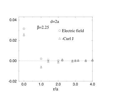
Figure 1: Electric field and curl of monopole currents in the confined phase for the Polyakov gauge.

However it can be shown [8] that this is the only sensible prescription; if one tries to recover the usual $U(1)$ behavior of the Polyakov line by rotating $\hat{\phi}$ in the $+$ and $-$ direction with the same statistical weight then any correlation between Abelian Wilson loops vanishes. Since we want to represent a quark-antiquark source at finite temperature with two Abelian Polyakov lines, $P_{1}P_{2}^{\ast}=e^{i(\theta_{1}-\theta_{2})}$, we have to solve the problem that $P_{1}P_{2}^{\ast}$ acquires a non-vanishing real part from the above described kinematical effect ($\theta$ is distributed, according to the Haar measure, as $\sin^{2}\theta$). Our solution is to define the quark-antiquark source as the connected part of the product of two Polyakov lines:

$$\langle P_{1}P_{2}\rangle-\langle P_{1}\rangle\langle P_{2}\rangle$$ (2)

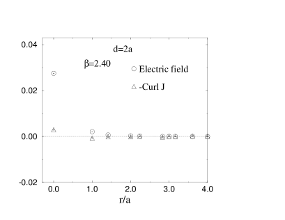
Figure 2: As in Fig. 1 but in the unconfined phase.

3 Measurements and discussion

We want to find direct evidence for the existence of dual Abrikosov vortices in the confined phase of the Abelian projected theory in the Polyakov gauge. Therefore we study the distribution of the electric field and of the monopole current around Abelian static sources, defined according to the procedure described in the previous section. Our aim is to interpret the results in terms of the dual superconductivity parameters i.e. the dual coherence length $\xi_{d}$ and the dual London penetration depth $\lambda_{d}$. We take our measurements at finite temperature on a $12^{3}\times 4$ lattice. The longitudinal electric field and the curl of the magnetic monopole current between static charges are defined as in [4]. In Fig. 1 we show the results in the confined phase ($\beta=2.25$) in the case of two sources separated by a distance $d=2$ in lattice spacings. We see a clear signal for both the electric field and the curl of the monopole currents on the axis of the two charges. As we move in the transverse direction $r$, we observe a rapid fall-off of the electric field while the monopole current shows a behavior consistent with the prediction of the dual Ginzburg-Landau theory. In Fig. 2 we show the results in the unconfined phase ($\beta=2.40$). In this case, the magnetic currents are much smaller and are consistent with zero in the region away from the axis of the two charges; moreover the electric field approaches zero less rapidly altough not clearly evident from the figure. Our conclusion is that dual vortices are present in the confined phase and disappear in the unconfined phase; hence we bring support to the dual superconductivity scenario in the Polyakov gauge [6].

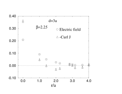
Figure 3: Electric field and monopole currents in the maximal Abelian gauge.

As already mentioned, similar results have been reported for the maximal Abelian gauge [4, 5]. In Fig. 3 we show the results in this gauge for the confined phase and $d=3a$. There are two main differences between these results and the correspondent results in the Polyakov gauge. First, the data in the maximal Abelian gauge support a non vanishing value for the coherence length $\xi_{d}$, while there is no evidence for it being different from zero in the Polyakov gauge. Then, the peak values of the electric field and the magnetic currents are more than an order of magnitude smaller in the Polyakov gauge than the correspondent values in the maximal Abelian gauge. We interpret these differences in terms of a different role played by the charged coset fields in the two projections. Specifically, we measure the spatial distribution of the electric charge in the region between two static sources. This can be done measuring the divergence of the electric field defined, at site $x$, as

$$\sum_{i=1}^{3}\frac{\langle\sin\theta_{PP^{\dagger}}(\sin\theta_{i4}(x)-\sin\theta_{i4}(x-i))\rangle}{a^{3}e\langle\cos\theta_{PP^{\dagger}}\rangle}$$ (3)

Figure 4: Divergence of the electric field along the axis connecting two static charges.

In Fig. 4 we show the results for two Polyakov lines separated by three lattice spacings. The figure clearly shows that the effective static charge is much smaller in the Polyakov gauge and that for $d\neq 0$ the coset fields in the two prescriptions respond in opposite ways to the presence of an electric charge.

Our conclusion is that dual vortices are present in the Polyakov gauge but are suppressed with respect to the maximal Abelian gauge due to the charged coset fields that are far more effective in shielding the electric charge in the case of the Polyakov gauge.

References

- [1] For a review and further references see e.g. R.W. Haymaker, lectures given at the International School of Physics “E. Fermi”, Varenna, 1995, hep-lat/9510035.
- [2] G. ’t Hooft, Nucl. Phys. B 190 (1981) 455.
- [3] M.N. Chernodub, M.I. Polikarpov and A.I. Veselov, preprint ITEP-TH-14-95.
- [4] V. Singh, D.A. Browne and R.W. Haymaker, Phys. Lett. B 306 (1993) 115.
- [5] P. Cea and L. Cosmai, Phys. Rev. D 52 (1995) 5152.
- [6] L. Del Debbio, A. Di Giacomo, G. Paffuti and P. Pieri, Phys. Lett. B 355 (1995) 255.
- [7] A.S. Kronfeld, G. Schierholz and U.J. Wiese, Nucl.Phys. B 293 (1987) 461.
- [8] K. Bernstein, G. Di Cecio and R.W. Haymaker, preprint LSUHE No. 213-1996.