HU-TFT-96-27

hep-lat/9607023

July 8, 1996

Dimensionally reduced U(1)+Higgs theory in the broken phase

Mika Karjalainen¹ and Janne Peisa²

Department of Physics
P.O. Box 9
FIN-00014 University of Helsinki, Finland

Abstract

We apply dimensional reduction to the finite temperature U(1)+Higgs theory and study the properties of the reduced 3-dimensional theory in the broken phase using lattice Monte Carlo simulations. We compute analytically the scalar condensate in optimized 2-loop perturbation theory and the correlators in 1-loop perturbation theory. These quantities are also calculated numerically. The two results for the condensate agree well but a 25% difference is observed for the scalar correlator, indicating the need for optimized 2-loop perturbative results.

1 Introduction

The U(1)+Higgs theory has been studied extensively in four dimensions [1, 2, 3], but only to a limited extent in 3d [4]. The 3d studies are mainly motivated by the fact that the theory then is directly the Ginzburg-Landau model of superconductivity. That the 3d theory also arises as an effective theory of the finite $T$ 4d U(1)+Higgs theory is a strong additional motivation to study it. Although the really physical case is the SU(2)+Higgs theory, it is nevertheless of great interest to investigate how changing the group from SU(2) to U(1) changes the dynamics. This may also help in understanding the phenomena in the full SU(2)$\times$U(1) standard model. The purpose of this article is to study the 3d U(1)+Higgs theory, mainly in the broken phase and for values of the couplings which are appropriate when the 3d theory is an effective theory of the finite $T$ 4d U(1)+Higgs theory [2, 3].

Perturbation theory in U(1)+Higgs model breaks down at the tree-level critical temperature, as the expansion parameter diverges when $T\to T_{c}$. Although the lattice $T_{c}$ differs slightly from the perturbative one, these temperatures are so close that perturbation theory is not valid at the lattice $T_{c}$ either. At temperatures below $T_{c}$, but still higher than all the mass scales in the theory, the expansion parameter is small and one expects that perturbation theory works rather well there. The main goal of this article is to make statements on the accuracy of perturbation theory at intermediate temperatures, where the expansion parameter is not too large and also try to estimate the temperature, at which perturbation theory is not valid anymore. To this end we compute on the one hand analytically in perturbation theory and on the other hand numerically with lattice Monte Carlo techniques the scalar condensate and the scalar and vector correlators. A comparison of the results gives a quantitative assessment of the accuracy of perturbation theory. We shall in a later paper [5] study the phase transition properties of the theory.

The accuracy of perturbation theory depends not only on the number of the loops but also on the optimization method used. In this paper we compare ordinary $\hbar$-expansion with another optimized method, namely the CW-method. The latter can also be applied when the broken minimum is radiatively generated, the first one requires the existence of the broken minimum already in the tree potential.

First we use the dimensional reduction to obtain an effective model for 4d finite temperature U(1)+Higgs theory. The idea of dimensional reduction is to integrate out all the non-zero Matsubara modes which are heavy at high temperature [6, 7]. The effective 3d theory obtained after reduction provides an excellent approximation of the original theory [3] when two basic conditions are satisfied: the coupling constants are small, so that we can relate the parameters of the original 4d and the effective 3d models pertubatively and $T$ is larger than all the relevant mass scales in the theory [8, 9]. Dimensional reduction has one major advantage over direct finite temperature 4d simulations. In particular the dimensionally reduced 3d theory contains less mass scales than the original theory (if we integrate over the temporal component of the gauge-field, there are two mass scales less), resulting in a huge gain in computer simulations. Because all fermions are integrated out at the reduction process, one could also study the theories with chiral fermions, which are problematic on the lattice in 4d.

To be able to compare our non-perturbative Monte Carlo data with perturbative results, we have to determine relevant observables accurately. An essential ingredient when comparing the perturbation theory to lattice calculations are the continuum-lattice mapping formulae, which are exact in 3d [10]. Thus the continuum limit can be carried out under controlled conditions.

2 Dimensional reduction

The Lagrangian of the 4d U(1)+Higgs theory at finite temperature without fermions is in standard notation

$${\cal L}=\frac{1}{4}F_{\mu\nu}F_{\mu\nu}+\left(D_{\mu}\phi\right)^{\ast}\left(D_{\mu}\phi\right)+m^{2}\phi^{\ast}\phi+\lambda\left(\phi^{\ast}\phi\right)^{2}.$$ (1)

One could also include fermions as this results in the same final effective 3d theory but with different parameter values.

In the following we shall choose the four dimensional coupling $g=1/3$ and the 4d tree masses $m_{H}=-2m^{2}=30,35,60$ GeV and $m_{W}=m_{H}\sqrt{g/2\lambda}=80.6$ GeV. We call the arbitary mass parameter $m_{H}$ the tree-level Higgs mass. The choice of these values of $m_{H}$ is motivated by the fact that for smaller values the transition becomes too strong for dimensional reduction to be accurate and for larger values perturbation theory becomes increasingly unreliable

The dimensional reduction of U(1)+Higgs theory is presented in [2] and we just collect the results here. After integrating over the scale $\pi T$ the typical scale of remaining 3d theory is $\sim g^{2}T$. There is still an adjoint Higgs field $A_{0}$ present in the theory, but its mass $m_{A_{0}}\sim gT$ is large compared with the scale of the theory. Hence also $A_{0}$ can be integrated out perturbatively. The action which is obtained after eliminating all heavy degrees of freedom is

$$S_{\mbox{\scriptsize eff}}\left[A_{i}({\bf x}),\phi_{3}({\bf x})\right]=\int d^{3}x\bigg{[}\frac{1}{4}F_{ij}F_{ij}+(D_{i}\phi_{3})^{2}+m_{3}^{2}\phi_{3}^{\ast}\phi_{3}+\lambda_{3}\left(\phi_{3}^{\ast}\phi_{3}\right)^{2}\bigg{]}.$$ (2)

The relations between 3d and 4d parameters are:

$$g_{3}^{2}=g^{2}(\mu)T,$$ (3)

$$\lambda_{3}=\lambda(\mu)T-\frac{g_{3}^{4}}{8\pi m_{D}},$$ (4)

$$m_{3}^{2}(\mu_{3}) = \bigg{[}\frac{1}{4}g_{3}^{2}T+\frac{1}{3}\lambda_{3}T+\frac{g_{3}^{2}}{16\pi^{2}}\left(-\frac{8}{9}g_{3}^{2}+\frac{2}{3}\lambda_{3}\right)\bigg{]}$$ (5)

$$-\frac{1}{2}m_{H}^{2}+{f_{2m}\over 16\pi^{2}}\left(\log{3T\over\mu_{3}}+c\right)$$

$$-\frac{g_{3}^{2}m_{D}}{4\pi}-\frac{g_{3}^{4}}{8\pi^{2}}\left(\log\frac{\mu_{3}}{2m_{D}}+\frac{1}{2}\right),$$

where we have

$$m_{D}^{2}=\frac{1}{3}g^{2}(\mu)T^{2},$$ (6)

$$f_{2m}=-4g_{3}^{4}+8\lambda_{3}g_{3}^{2}-8\lambda_{3}^{2}.$$ (7)

The constant $c=-0.348725$.

The mean field dependent masses are

$$m_{T}=g_{3}\phi, m_{1}^{2}=m_{3}^{2}(\mu_{3})+3\lambda_{3}\phi^{2}, m_{2}^{2}=m_{3}^{2}(\mu_{3})+\lambda_{3}\phi^{2}.$$ (8)

The couplings $g_{3}^{2}$ and $\lambda_{3}$ are 3d renormalization group invariant. When propagators are calculated perturbatively we notice that the mass parameter $m_{3}^{2}$ contains both linear and logaritmic divergences. The appearance of a logarithmic divergence introduces a scale $\mu_{3}$ into our theory. We can choose this extra scale to be the scale parameter of dimensional regularization in 3d $\overline{\rm MS}$ scheme. The tree parameters must be transformed with renormalization group equations when $\mu_{3}$ varies if we want to keep the physical content of the theory unchanged.

All the information of the 4d theory is contained in just three parameters: a dimensionful gauge coupling constant $g_{3}^{2}$, which defines the typical scale of the system and two dimensionless numbers which we define as

$$x\equiv\frac{\lambda_{3}}{g_{3}^{2}},\,\,\,\,y\equiv\frac{m_{3}^{2}(g_{3}^{2})}{g_{3}^{4}}.$$ (9)

The parameter $x$ is essentially proportional to the ratio of the squares of the scalar and vector masses in the broken phase, while $y$ is related to the temperature, $y\sim(T-T_{c})/T_{c}$, so that at tree level $y=0$ describes the phase transition point. In terms of 4d parameters they can be expressed as

$$x=\frac{1}{2}\frac{m_{H}^{2}}{m_{W}^{2}}-\frac{\sqrt{3}g}{8\pi},$$ (10)

$$y = \frac{1}{4g^{2}}+\frac{1}{3}\left(x+\frac{\sqrt{3}g}{8\pi}\right)\frac{1}{g^{2}}+\frac{1}{16\pi^{2}}\left[-\frac{8}{9}+\frac{2}{3}\left(x+\frac{\sqrt{3}g}{8\pi}\right)\right]$$ (11)

$$-\frac{1}{4\pi\sqrt{3}g}-\frac{1}{8\pi^{2}}\left(\log\frac{3\sqrt{3}}{2g}+c+\frac{1}{2}\right)-\frac{m_{H}^{2}}{2g^{4}T^{2}}$$

$$+\frac{1}{16\pi^{2}}\left(-4+8x-8x^{2}\right)\left(\log\frac{3}{g^{2}}+c\right).$$

The 4d tree level Higgs mass values $m_{H}=30,35$ and $60$ GeV correspond to $x=0.0463,0.0713$ and $x=0.254$ according to equation (10).

3 Perturbative calculation of the properties of the system in the broken phase

3.1 3d effective potential

The tree potential is obtained from the Lagrangian (2)

$$V_{0}={1\over 2}m_{3}^{2}\phi^{2}+{1\over 4}\lambda_{3}\phi^{4},$$

and the 1-loop part of the effective potential in 3d is

$$V_{1}=-\frac{1}{12\pi}\left[2m_{T}^{3}+m_{1}^{3}+m_{2}^{3}\right].$$ (12)

The 2-loop potential in 3d contains diagrams in Fig. 1 ($\times 1/(16\pi^{2})$)

$$(a) = -g^{4}\phi^{2}D_{VVS}(m_{T},m_{T},m_{1}),$$

$$(c) = -\lambda^{2}\phi^{2}\left[3H(m_{1},m_{1},m_{1})+H(m_{1},m_{2},m_{2})\right],$$

$$(f1) = -\frac{1}{2}g^{2}D_{SSV}(m_{1},m_{2},m_{T}),$$

$$(f2) = g^{2}m_{T}(m_{1}+m_{2}),$$

$$(h4) = \frac{1}{4}\lambda\left(3m_{1}^{2}+2m_{1}m_{2}+3m_{2}^{2}\right),$$ (13)

where we have used the results and diagram notations of [2] and

Figure 1: The 2-loop diagrams contributing to the 3d effective potential.

$$D_{SSV}(m_{1},m_{2},M) = \left(M^{2}-2m_{1}^{2}-2m_{2}^{2}\right)H(M,m_{1},m_{2})$$ (14)

$$+\frac{\left(m_{1}^{2}-m_{2}^{2}\right)^{2}}{M^{2}}[H(M,m_{1},m_{2})-H(0,m_{1},m_{2})]$$

$$+\frac{1}{M}{(m_{1}+m_{2})\left[M^{2}+(m_{1}-m_{2})^{2}\right]-Mm_{1}m_{2}},$$

$$D_{VVS}(M,M,m) = \bigg{(}2H(M,M,m)-\frac{1}{2}H(M,m,0)+\frac{m^{2}}{M^{2}}[H(M,m,0)$$ (15)

$$-H(M,M,m)]+\frac{m^{4}}{4M^{4}}[H(m,0,0)+H(M,M,m)$$

$$-2H(M,m,0)]-{m\over 2M}-{m^{2}\over 4M^{2}}\bigg{)},$$

$$H(m_{1},m_{2},m_{3})=\log\frac{\mu_{3}}{m_{1}+m_{2}+m_{3}}+\frac{1}{2}.$$ (16)

3.2 Choosing the scale

As discussed previously the only scale dependent parameter in this theory is the mass parameter $m_{3}^{2}(\mu_{3})$, as the coupling constants do not run. We also know that the effective potential is scale independent to a certain order. On the other hand for example the tree as well as the 2-loop effective potentials on their own are explicitly $\mu_{3}$ dependent, the scale dependence cancels to this order when they are combined. The question is now, how to choose the scale so that the higher order loop corrections are small and predictions of physical parameters can be made.

In many theories, including this, the problem involves large logarithms. The 2-loop effective potential, which carries the logarithms is only weakly $\mu_{3}$ dependent. One should choose the scale so that the effect of these logarithmic terms is minimized and it is quite natural to achieve this by demanding that the 2-loop contribution vanishes totally. This is not exactly sufficient because the effective potential is not renormalization group invariant, it is not a physical quantity. Only the difference $V(\phi_{1})-V(\phi_{2})$ is measurable. One should then really look at the derivative $dV/d\phi$, which is $\mu_{3}$ independent.

In the effective U(1)+Higgs theory we have three different mass scales ($m_{T},m_{1},m_{2}$) and the determination of proper $\mu_{3}$ is nontrivial. Let’s first assume that $m_{T}\gg m_{1},m_{2}$ so the Higgs mass is so small that we can neglect the $m_{1}$ and $m_{2}$ terms. Solving then $dV_{2}=0$ we find that the choice of $\mu_{3}$ which minimizes the 2-loop potential is

$$\mu_{3}=\kappa m_{T},$$ (17)

where $\kappa$ has to be determined using some other criterion of minimizing the effect of 2-loop terms. Here we demand that the value of $\phi$ at the critical temperature $T_{c}$ is the same for the 1-loop and 2-loop potentials in the broken phase. This parametrization with constant $\kappa$ works rather well, when the Higgs mass is small. When all three mass scales ($m_{T},m_{1},m_{2}$) are included, we generalize (17) by choosing

$$\mu_{3}(\phi)=\kappa(\phi)m_{T},$$ (18)

where $\kappa(\phi)$ is fitted numerically at every point $\phi$ so that the derivative of the 2-loop contribution vanishes. Pictures of potentials with different Higgs masses are presented in Figures 2 and 3. The corresponding $\kappa(\phi)$:s can be seen in Figure 4. Note that the value of $\kappa(\phi)$ and therefore also $\mu_{3}(\phi)$ is not well determined for very small values of $\phi$ because perturbation theory is not valid there.

Figure 2: The renormalization group improved 2-loop potential near the phase transition point, with $m_{H}=35$ GeV.

Figure 3: The 2-loop potential with $m_{H}=60$ GeV.

Figure 4: Fitted $\kappa(\phi)$:s with $m_{H}=35$ GeV, $T=148.83$ GeV $\approx T_{c}$ and $m_{H}=60$ GeV, $T=226.77$ GeV $\approx T_{c}$.

3.3 The ground state energy and the scalar condensate in the broken phase

We will now calculate analytically the ground state energy of the theory and the scalar condensate using methods described in [3, 14].

In perturbation theory the effective potential is derived as an expansion where the expansion parameter is the Planck constant $\hbar$

$$V(\phi)=\sum_{n=0}^{N}\hbar^{n}V_{n}(\phi).$$ (19)

Although the potential is gauge dependent, its value in the broken minimum, which gives the vacuum expectation value $\nu(T)$ of $\phi$ is gauge independent and determined by

$$\left.\sum_{n=0}^{N}\hbar^{n}\frac{dV_{n}(\phi)}{d\phi}\right|_{\phi=\nu(T)}=0.$$ (20)

The aim is now to solve $\nu(T)$ from (20).

We look at the so called ”classical” regime, where spontaneous symmetry breaking occurs already on the tree-level of the potential. This means that there is a (non-trivial) solution $\nu_{0}^{2}(T)=-m_{3}^{2}/\lambda_{3}$ so that

$$\left.\frac{dV_{0}(\phi)}{d\phi}\right|_{\phi=\nu_{0}(T)}=0,$$ (21)

which gives the leading approximation to $V_{min}$

$$V_{min}\sim V_{0}(\nu_{0})=-\frac{m^{4}_{3}}{4\lambda_{3}}.$$ (22)

If perturbation theory works well we can use this saddle point value as a good start ($\nu(T)=\nu_{0}(T)+{\cal O}(\hbar)$) and solve (20) perturbatively

$$\varphi=\sum_{n=0}^{N}\hbar^{n}\varphi_{n},$$ (23)

where we have denoted $\varphi=\nu^{2}(T)$ and $\varphi_{0}=\nu_{0}^{2}(T)$.

Perturbation theory works only when the expansion parameter is small enough. When we look at 1-loop and 2-loop potentials separately we notice that typical 1-loop terms have $m_{T}^{2}/2\pi$ with them and 2-loop terms include $g_{3}^{2}m_{T}^{2}/(2\pi)^{2}$. The expansion parameter $\rho$ is the ratio of these

$$\rho=\frac{g_{3}^{2}}{2\pi m_{T}}=\sqrt{\frac{g_{3}^{2}\lambda_{3}}{-m_{3}^{2}\pi}}.$$ (24)

So the ”classical” regime approximation is valid when

$$m_{3}^{2}<0, |m_{3}^{2}|\gg g_{3}^{2}\lambda_{3}.$$ (25)

Using (19) and (23) we have at the minimum

$$V^{\prime}_{0}(\varphi_{0}+\hbar\varphi_{1}+\hbar^{2}\varphi_{2})$$

$$+\hbar V^{\prime}_{1}(\varphi_{0}+\hbar\varphi_{1})+\hbar^{2}V^{\prime}_{1}(\varphi_{0})+{\cal O}(\hbar^{3}) = 0.$$ (26)

Here primes mean that we take partial derivatives with respect to $\phi^{2}$ and evaluate the expression at the value written in parenthesis. When we also expand all $V_{n}$:s near $\varphi_{0}$ we get

$$V^{\prime}_{0}(\varphi_{0})+V^{\prime\prime}_{0}(\varphi_{0})[\hbar\varphi_{1}+\hbar^{2}\varphi_{2}]$$

$$+\frac{1}{2}V^{\prime\prime\prime}_{0}(\varphi_{0})[\hbar^{2}\varphi^{2}_{1}]+\hbar V^{\prime}_{1}(\varphi_{0})$$

$$+\hbar V^{\prime\prime}_{1}(\varphi_{0})[\hbar\varphi_{1}]+\hbar^{2}V^{\prime}_{2}(\varphi_{0})+{\cal O}(\hbar^{3}) = 0.$$ (27)

All degrees of $\hbar$ must vanish separately, which gives

$$\varphi_{1}=-\frac{V^{\prime}_{1}(\varphi_{0})}{V^{\prime\prime}_{0}(\varphi_{0})}.$$ (28)

From now on we will not write down the $\varphi_{0}$-term any more, although all potential terms are still evaluated at this saddle point.

The value of the effective potential at the minimum up to 3 loops is calculated by expanding (19) with (23)

$$V_{min} = V_{0}+\hbar V_{1}+\hbar^{2}\left[V_{2}+\frac{1}{2}V^{\prime}_{1}\varphi_{1}\right]$$ (29)

$$+\hbar^{3}\left[V_{3}+V^{\prime}_{2}\varphi_{1}+\frac{1}{2}V^{\prime\prime}_{1}\varphi^{2}_{1}\right]+{\cal O}(\hbar^{4}),$$

which gives the ground state energy in the broken phase. With this, we can easily calculate the scalar condensate $\langle\phi^{\ast}\phi(\mu_{3})\rangle$ in the broken phase

$$\langle\phi^{\ast}\phi(\mu_{3})\rangle=\frac{dV_{min}}{dm_{3}^{2}(\mu_{3})}.$$ (30)

Although the 3d-effective potential is calculated only up to 2-loops, we can make some predictions of the 3-loop potential term.

There is a 3-loop order logaritmic $\mu_{3}$-dependence in the 1-loop potential $V_{1}$ because of the $\mu_{3}$-dependence of $m_{1}(\phi)$. Because the 3-loop level effective potential is $\mu_{3}$-independent, there must be a term in $V_{3}$ which cancels this. So, $V_{3}$ must include a term

$$V_{3a} = -\mu_{3}\frac{\partial V_{1}}{\partial\mu_{3}}\left[\log\frac{\mu_{3}}{m_{T}}+\frac{1}{2}\right]$$ (31)

$$= \frac{\partial V_{1}}{\partial m_{3}^{2}}\frac{f_{2m}}{16\pi^{2}}\left[\log\frac{\mu_{3}}{m_{T}}+\frac{1}{2}\right],$$

and a $\mu_{3}$-dependence of $V_{1}+V_{3}$ is of order $\hbar^{5}$. When we calculate the ground state energy the last term of (29) gives a term proportional to $1/m_{2}$. At the saddle point $m_{2}\rightarrow 0$ and this term diverges. To avoid this, there must be another compensating term in $V_{3}$. Calculation of $V^{\prime}_{2}\varphi_{2}+\frac{1}{2}V^{\prime\prime}_{1}\varphi^{2}_{1}$ gives us this term

$$V_{3b}=\frac{1}{32}\left(4+3r^{3}\right)^{2}\frac{g_{3}^{4}}{(4\pi)^{3}}\frac{m^{2}_{T}}{m_{2}},$$ (32)

where

$$r^{2}\equiv\frac{2\lambda_{3}}{g_{3}^{2}}.$$ (33)

There will be other contributions also, which for pure scalar theory have been explicitly computed by [15]. In SU(2)+Higgs theory this unknown information was included under one linear term [2], which can be derived just on dimensional grounds. This term depends on masses, $\phi$ and a dimensionless constant parameter $\beta$

$$V_{3c}=\rho\frac{m^{2}_{T}}{2\pi}\beta=\frac{g_{3}^{4}m_{T}}{(4\pi)^{3}}\beta.$$ (34)

In U(1)+Higgs theory this kind of linear term is absent [11] so the unknown part cannot be found using this parametrization.

The known part of the 3-loop potential $V_{3}$ can be written in form

$$V_{3} = V_{3a}+V_{3b}$$ (35)

$$= \frac{\partial V_{1}}{\partial m_{3}^{2}}\frac{f_{2m}}{16\pi^{2}}\left[\log\frac{\mu_{3}}{m_{T}}+\frac{1}{2}\right]+\frac{1}{32}\left(4+3r^{2}\right)^{2}\frac{g_{3}^{4}}{(4\pi)^{3}}\frac{m^{2}_{T}}{m_{2}}.$$

To be able to calculate the scalar condensate we must now find $V_{min}$ explicitly. First we have to calculate $\varphi_{0}$ and $\varphi_{1}$. Using (28) with (12) and (13), we get

$$\varphi_{0} = \frac{-m_{3}^{2}(\mu_{3})}{\lambda_{3}}$$ (36)

$$\varphi_{1} = \frac{1}{4\pi r^{2}}\left(4m_{T}+3m_{1}r^{2}+m_{2}r^{2}\right)={3\over 4\pi}\left({4\over r^{2}}+r\right)m_{T},$$ (37)

where masses are evaluated at the saddle point

$$m_{1}=rm_{T}=\sqrt{-2m_{3}^{2}(\mu_{3})},\hskip 14.22636ptm_{2}=0,$$ (38)

and

$$\frac{dm_{T}}{dm_{3}^{2}}=-\frac{1}{r^{2}m_{T}},\hskip 14.22636pt\frac{dm_{1}}{dm_{3}^{2}}=-\frac{1}{m_{1}}.$$ (39)

Inserting these into the potentials we get

$$V_{0} = -\frac{m_{3}^{4}(\mu_{3})}{\lambda_{3}},$$ (40)

$$\vspace*{0.3cm}V_{1} = -\frac{1}{12\pi}\left(2+r^{2}\right)m_{T},$$ (41)

$$\vspace*{0.3cm}V_{2}+\frac{1}{2}V^{\prime}_{1}\varphi_{1} = \frac{1}{16\pi^{2}}g_{3}^{2}m_{T}^{2}\left[f_{1}(r)\left(\log\frac{\mu_{3}}{m_{T}}+\frac{1}{2}\right)+q_{1}(r)\right],$$ (42)

where

$$f_{1}(r) = -\left(2-r^{2}+r^{4}\right),$$ (43)

$$\vspace*{0.3cm}q_{1}(r) = \left(2-r^{2}+\frac{1}{4}r^{4}\right)\log(2+r)-2r+\frac{1}{4}r^{4}$$ (44)

$$-\frac{1}{2}r^{3}+\frac{3}{4}r^{4}\log(3r)-\frac{2}{r^{2}}-\frac{3}{4}r^{4}.$$

Now a lengthy computation shows that

$$V^{\prime}_{2}\varphi_{1}+\frac{1}{2}V^{\prime\prime}_{1}\varphi_{1}^{2} = \frac{3}{2}\left(r+\frac{4}{3r^{2}}\right)\frac{m_{T}f_{2m}}{(4\pi)^{3}}\left(\log\frac{\mu_{3}}{m_{T}}+\frac{1}{2}\right)$$ (45)

$$+\beta_{disc}(r)\frac{m_{T}g_{3}^{4}}{(4\pi)^{3}}$$

$$+\frac{1}{32}\left(4+3r^{3}\right)^{2}\frac{g_{3}^{4}}{(4\pi)^{3}}\frac{m_{T}^{2}}{m_{2}},$$

where the divergent $m_{2}$ part cancels with $V_{3}$ and

$$\beta_{disc}(r) = {4+3r^{3}\over 32r^{4}(2+r)}\bigg{[}-64-32r+64r^{2}+8r^{3}-36r^{4}-40r^{5}+10r^{6}$$ (46)

$$+13r^{7}+(48r^{6}+24r^{7})\log(3)+(64r^{6}+32r^{7})\log(r)$$

$$-(32r^{4}+16r^{5}+32r^{6}+16r^{7})\log(1+r)$$

$$+(128r^{2}+64r^{3}-96r^{4}-48r^{5}+32r^{6}+16r^{7})\log(2+r)\bigg{]}.$$

Using (35) and inserting these into (29) gives us the vacuum energy density in the broken phase up to 3-loops

$$V_{min} = -\frac{m_{3}^{4}(\mu_{3})}{\lambda_{3}}-\frac{1}{12\pi}\left(2+r^{2}\right)m_{T}$$ (47)

$$+\frac{1}{16\pi^{2}}g_{3}^{2}m_{T}^{2}\left[f_{1}(r)\left(\log\frac{\mu_{3}}{m_{T}}+\frac{1}{2}\right)+q_{1}(r)\right]$$

$$+\left(r+\frac{2}{r^{2}}\right){m_{T}f_{2m}\over(4\pi)^{3}}\left(\log\frac{\mu_{3}}{m_{T}}+\frac{1}{2}\right)$$

$$+{m_{T}g_{3}^{4}\over(4\pi)^{3}}\beta_{disc}(r).$$

To be able to compare the perturbative results with Monte Carlo data we must calculate the analytic form of scalar condensate $\langle\phi^{\ast}\phi\rangle$. This is easily done using (30). In terms of previously defined parameters $x$ and $y$ the condensate is

$${\langle\phi^{\ast}\phi(\mu_{3})\rangle\over g_{3}^{2}} = {-y(\mu_{3})\over 2x}+{1\over 4\pi}\left(r+{2\over r^{2}}\right)m_{T}$$ (48)

$$-{1\over x}{1\over 16\pi^{2}}\left[f_{1}(r)\log\frac{\mu_{3}}{m_{T}}+q_{1}(r)\right]$$

$$-{g_{3}^{2}\over(4\pi)^{3}}{1\over r^{2}m_{T}}\bigg{[}{f_{2m}\over g_{3}^{4}}\left(r+{2\over r^{2}}\right)\left(\log{\mu_{3}\over m_{T}}-{1\over 2}\right)$$

$$+\beta_{disc}(r)\bigg{]},$$

where $m_{T}$ is

$$m_{T}=g_{3}^{2}\sqrt{\frac{-y(\mu)}{x}}$$ (49)

and

$$y(\mu)=y+\frac{1}{16\pi^{2}}\left(-4+8x-8x^{2}\right)\log\frac{g_{3}^{2}}{\mu}.$$ (50)

3.4 Coleman-Weinberg method

The direct $\hbar$ expansion discussed above for calculating the scalar condensate is not valid at the phase transition point because the expansion parameter $\rho$ diverges. It also has higher order $\mu_{3}$-dependence, which is significant near the critical temperature. We can mainly avoid these problems using another, so called Coleman-Weinberg (CW) method which is much less scale dependent and can be used even beyond the critical temperature. With the CW method one numerically determines the location of the broken minimum $\varphi_{0}(T)$ of the renormalization group improved 2-loop effective potential and then calculates the ground state energy of the system. Finally one computes the condensate using equation (30). Because of the singularities at the classical tree-level minimum ($V_{3}\sim 1/m_{2}$ and $m_{2}\to 0$), the ground state energy computed by CW-method differs from the result of the straightforward $\hbar$-expansion. One should then redefine the 2-loop potential by including all leading singularities in it (Appendix B in [14]). This should not be a major problem in this case, because the difference is of order $\hbar^{\frac{5}{2}}$ and we have the effective potential only up to $\hbar^{2}$ as there are still unknown parts in the $\hbar^{3}$-level.

$T$	106.4	115.8	125.4	126.8	127.5
$\langle\phi^{\ast}\phi\rangle/T$	2.395(6)	1.551(8)	0.807(4)	0.705(11)	0.638(5)
$\hbar$-exp.	2.369(6)	1.515(9)	0.707(20)	0.573(27)	0.495(37)
CW	2.392(2)	1.550(1)	0.784(2)	0.672(2)	0.614(2)

Table 1: Measured and computed values of $\langle\phi^{\ast}\phi\rangle/T$ for $m_{H}=30$ GeV. The first row gives the lattice value extrapolated to continuum limit. The last two rows show the 2-loop perturbative values using both $\hbar$ expansion and CW-optimization. The errors on the perturbative values are obtained by varying the scale parameter $\mu$ as indicated in the text.

The results with both of these methods are presented in section 4. The remaining $\mu_{3}$-dependence of the CW-method can be used to measure the accuracy of the calculation. We fix the scale $\mu_{3}$ so that the convergence of perturbation theory is maximized near the minimum with a method discussed in chapter 3.2. We vary this fixed scale used in the calculation of $\langle\phi^{\ast}\phi(\mu_{3})\rangle$ within limits $0.5\mu_{\mbox{\scriptsize fix}}<\mu_{3}<2\mu_{\mbox{\scriptsize fix}}$. To compare these results with the Monte Carlo data we must also run $\langle\phi^{\ast}\phi(\mu_{3})\rangle$ to $\mu_{3}=g_{3}^{2}$ using the running

$$\langle\phi^{\ast}\phi(\mu_{1})\rangle-\langle\phi^{\ast}\phi(\mu_{2})\rangle=\frac{g_{3}^{2}}{8\pi^{2}}\log\frac{\mu_{1}}{\mu_{2}}.$$ (51)

Table 1 shows that the CW-values of the scalar condensate are almost independent of $\mu_{3}$ and thus more accurate than the results calculated with $\hbar$ expansion.

3.5 Propagators and particle masses

The perturbative masses of the system are derived as poles of the corresponding propagators. Here we calculate the scalar and vector propagator up to 1-loop level. The propagators are

$$\langle\phi_{1}(-k)\phi_{1}(k)\rangle = \frac{1}{k^{2}+m_{1}^{2}-\Pi^{S}(k^{2})},$$ (52)

$$\langle A_{i}(-k)A_{j}(k)\rangle = \frac{\delta_{ij}-\frac{p_{i}p_{j}}{p^{2}}}{k^{2}+m_{T}^{2}-\Pi^{V}(k^{2})}+\mbox{longitudinal}.$$ (53)

At 1-loop level the propagators contain diagrams in Fig. 5 and 6.

Figure 5: The 1-loop diagrams contributing to the scalar propagator.

The scalar self-energy is the sum of the following terms (Figure 5)

$$\Pi_{S}^{S} = \lambda_{3}\left[3A_{0}(m_{1}^{2})+A_{0}(m_{2}^{2})\right],$$ (54)

$$\Pi_{V}^{S} = 2g_{3}^{2}A_{0}(m_{T}^{2}),$$ (55)

$$\Pi_{SS}^{S} = 2\lambda_{3}^{2}\phi^{2}\left[9B_{0}(k^{2};m_{1}^{2},m_{2}^{2})+B_{0}(k^{2};m_{2}^{2},m_{2}^{2})\right],$$ (56)

$$\Pi_{VV}^{S} = \frac{g_{3}^{2}}{2m_{T}^{2}}\left\{B_{0}(k^{2};m_{T}^{2},m_{T}^{2})\left[k^{4}+4k^{2}m_{T}^{2}+8m_{T}^{4}\right]\right.$$ (57)

$$\left.-2B_{0}(k^{2};m_{T}^{2},0)\left[k^{2}+m_{T}^{2}\right]^{2}\right.$$

$$\left.+B_{0}(k^{2};0,0)k^{4}-2A_{0}(m_{T})^{2}m_{T}^{2}\right\},$$

$$\Pi_{SV}^{S} = \frac{g_{3}^{2}}{m_{T}^{2}}\left\{B_{0}(k^{2};m_{T}^{2},m_{2}^{2})\left[k^{4}+2k^{2}(m_{T}^{2}+m_{2}^{2})+(m_{T}^{2}-m_{2}^{2})^{2}\right]\right.$$ (58)

$$\left.-B_{0}(k^{2};m_{2}^{2},0)\left[k^{2}+m_{2}^{2}\right]^{2}\right.$$

$$\left.-A_{0}(m_{2}^{2})m_{T}^{2}+A_{0}(m_{T}^{2})\left[m_{T}^{2}-m_{2}^{2}-k^{2}\right]\right\},$$

where we have used the integrals

$$A_{0}(m^{2}) = \int\frac{d^{d}p}{(2\pi)^{d}}\frac{1}{p^{2}+m^{2}}=-\frac{m}{4\pi}$$ (59)

$$B_{0}(k^{2};m_{1}^{2},m_{2}^{2}) = \int\frac{d^{d}p}{(2\pi)^{d}}\frac{1}{[p^{2}+m_{1}^{2}][(p+k)^{2}+m_{2}^{2}]}$$ (60)

$$= \frac{i}{8\pi(k^{2})^{1/2}}\log\frac{m_{1}+m_{2}-i(k^{2})^{1/2}}{m_{1}+m_{2}+i(k^{2})^{1/2}}.$$

Figure 6: The 1-loop diagrams contributing to the vector propagator.

The vector self-energy contains the following parts (Figure 6)

$$\Pi_{S}^{V} = g_{3}^{2}\left[A_{0}(m_{1}^{2})+A_{0}(m_{2}^{2})\right],$$ (61)

$$\Pi_{SS}^{V} = -\frac{g_{3}^{2}}{2}\left\{B_{0}(k^{2};m_{1}^{2},m_{2}^{2})\left[k^{2}+2(m_{1}^{2}+m_{2}^{2})+\frac{(m_{1}^{2}-m_{2}^{2})^{2}}{k^{2}}\right]\right.$$ (62)

$$\left.\left[A_{0}(m_{1}^{2})-A_{0}(m_{2}^{2})\right]\frac{m_{1}^{2}-m_{2}^{2}}{k^{2}}-A_{0}(m_{1}^{2})-A_{0}(m_{2}^{2})\right\},$$

$$\Pi_{SV}^{V} = g_{3}^{2}\left\{B_{0}(k^{2};m_{T}^{2},m_{1}^{2})\left[-k^{2}-2m_{1}^{2}+6m_{T}^{2}-\frac{(m_{1}^{2}-m_{T}^{2})^{2}}{k^{2}}\right]\right.$$ (63)

$$\left.-B_{0}(k^{2};m_{1}^{2},0)\left[\frac{\left(k^{2}+m_{1}^{2}\right)^{2}}{k^{2}}\right]\right.$$

$$\left.+A_{0}(m_{T}^{2})\left[1+\frac{m_{1}^{2}-m_{T}^{2}}{k^{2}}\right]+A_{0}(m_{1}^{2})\frac{m_{T}^{2}}{k^{2}}\right\}.$$

The mean field dependent masses are evaluated at the minimum of the RG-improved 2-loop effective potential.

4 Monte Carlo simulations

The validity of perturbative results derived in previous section can be studied by performing Monte Carlo simulations of 3d U(1)+Higgs theory. Discretizing the continuum action (2) in the usual way one gets

$$S = \beta_{G}\sum_{\Box}\mbox{Re}(1-U_{\Box})$$ (64)

$$-\beta_{H}\sum_{{x},\mu}\mbox{Re}\left[\phi^{\ast}(x)U_{\mu}(x)\phi(x+\hat{\mu})\right]$$

$$+\sum_{{x}}\phi^{\ast}(x)\phi({x})+\beta_{R}\sum_{{x}}\left(1-\phi^{\ast}(x)\phi({x})\right)^{2},$$

where $U_{\mu}(x)$ is a gauge field located on the links of the lattice and $\phi(x)$ is a complex scalar field located on sites. $U_{\Box}$ is the product of gauge fields around a plaquette. This action has three coupling constants $\beta_{G},\beta_{H}$ and $\beta_{R}$, giving us a three dimensional parameter space. The continuum limit $a\to 0$ is described by the point $\beta_{G}=\infty,\beta_{H}=1/3,\beta_{R}=0$.

4.1 Constant physics curve

To be able to compare the results from our simulations with the continuum theory we have to establish the relation between lattice parameters $\beta_{G},\beta_{H}$ and $\beta_{R}$ and continuum parameters $x,y$ and $g_{3}^{2}$. This is done by a constant physics curve, which can be calculated using lattice perturbation theory. Due to the fact that the continuum couplings are dimensionful, an exact relation can be found with a 2-loop calculation [10]. The relevant relations are

$$\beta_{G} = {1\over ag_{3}^{2}},$$

$$\beta_{R} = {x\beta_{H}^{2}\over 4\beta_{G}},$$

$$2\beta_{G}^{2}\left({1\over\beta_{H}}-3-{2\beta_{R}\over\beta_{H}}\right) = y-(2+4x){\Sigma\beta_{G}\over 4\pi}$$ (65)

$$-{1\over 16\pi^{2}}\bigg{[}\left(-4+8x-8x^{2}\right)$$

$$\times\left(\ln 6\beta_{G}+0.09\right)+25.5+4.6x\bigg{]},$$

where $\Sigma=3.176$. We used $x=0.0463$ ,corresponding to $m_{H}=30$ GeV according to equation (10), in all simulations and varied the parameter $y$, which corresponds to temperature according to equation (11), between $-1$ and $-0.025$. At the lower end of this range perturbation theory is expected to work rather well, while approaching the critical point $y_{c}\simeq 0$ it should break down.

4.2 Algorithms used

By writing the Higgs field as $\phi(x)=R(x)e^{i\varphi(x)}$ and gauge field as $U_{\mu}(x)=e^{i\theta_{\mu}(x)}$, we obtain the following expression for action

$$S = \beta_{G}\sum_{x}\left(1-\cos\left(\theta_{\Box}\right)\right)$$ (66)

$$-\beta_{H}\sum_{{x},\mu}R(x)\cos\left(-\varphi(x)+\theta_{\mu}(x)+\varphi(x+\hat{\mu})\right)R(x+\hat{\mu})$$

$$+\sum_{{x}}R(x)^{2}+\beta_{R}\sum_{{x}}\left(1-R(x)^{2}\right)^{2}.$$

We used an overrelaxed heatbath algorithm for the gauge field. The heatbath algorithm used for the gauge field is described in [12]. This local heat bath was then combined with standard overrelaxation, where the angle is flipped to the other side of the minimum.

The form of the action would suggest separation of the radial and angular modes of the Higgs field, in which case one could by change of integration variables eliminate the angle of the Higgs field as a dynamical variable, thus possibly saving some computer time. However, the slow modes of the system are associated with the radius of the Higgs field and therefore it is essential to update radial part as efficiently as possible. The obvious overrelaxation algorithm [13] for the radial part of the Higgs field doesn’t improve the correlation time significantly. This is due to a rather poor acceptance ratio.

The best way to cope [14] with this problem seems to be not to separate the radial and angular update of the Higgs field, but rather update the cartesian components. This is done by defining two dimensional vectors

$${\bf r}=\left(\begin{array}[]{c}R\cos\varphi\\ R\sin\varphi\end{array}\right),$$ (67)

and

$${\bf v}=\left(\begin{array}[]{c}f\cos\theta\\ f\sin\theta\end{array}\right).$$ (68)

Now the local action

$$S_{\mbox{\scriptsize loc}}=fR\cos(\phi+\phi_{v})+c_{1}R^{2}+c_{2}R^{4},$$

can be written as

$$S_{\mbox{\scriptsize loc}}={\bf v\cdot r}+c_{1}R^{2}+c_{2}R^{4}.$$ (69)

If we now choose the components of the vector $\bf r$ perpendicular and orthogonal to $\bf v$, denoted by $x$ and $y$, we get

$$S_{\mbox{\scriptsize loc}}=fx+c_{1}(x^{2}+y^{2})+c_{2}(x^{2}+y^{2})^{2},$$ (70)

which suggests the following overrelaxation algorithm: first we update $y\to-y$, which corresponds to overrelaxation of the phase of the Higgs field, and then we solve the equation (70) to get a new value for $x$ leaving the action invariant.

For an exact overrelaxation algorithm one must leave the total path integral invariant, in this case this means that if we change $x$ to $x^{\prime}$ we should have

$${dS_{\mbox{\scriptsize loc}}(x)\over dx}^{-1}\exp(-S_{\mbox{\scriptsize loc}}(x))={dS_{\mbox{\scriptsize loc}}(x^{\prime})\over dx^{\prime}}^{-1}\exp(-S_{\mbox{\scriptsize loc}}(x^{\prime})).$$ (71)

Following [14] we now adopt an approximate method and choose $x^{\prime}$ so that the local action $S_{\mbox{\scriptsize loc}}$ is invariant and to accept this change with probability

$$p=\min({dS_{\mbox{\scriptsize loc}}(x^{\prime})\over dx^{\prime}}/{dS_{\mbox{\scriptsize loc}}(x)\over dx},1).$$ (72)

In our simulations the acceptance ratio was between 99.5 - 99.9%. This is similar to values reported in three dimensional simulations of SU(2)+Higgs theory [14].

The simulations were done using Cray C90 at Center of Scientific Computation in Helsinki.

4.3 Condensates

We concentrated mainly on the scalar condensate, for which the continuum and lattice normalizations are related by

$$\langle\phi^{\ast}\phi\rangle={\beta_{H}\over 2a}\langle R^{2}\rangle.$$ (73)

The 2-loop perturbative result calculated in $\overline{\rm MS}$ scheme is given by equation (48), which must be related to lattice regularization scheme. One gets [10]

$$\langle\phi^{\ast}\phi\rangle = {1\over 2}\beta_{H}\beta_{G}g_{3}^{2}\langle R^{2}\rangle-{g_{3}^{2}\beta_{G}\Sigma\over 4\pi}$$ (74)

$$-{g_{3}^{2}\over 8\pi^{2}}\left[\log(6\beta_{G})+\zeta+{\Sigma^{2}\over 4}-\delta\right],$$

where $\Sigma=3.176$, $\zeta=0.09$ and $\delta=1.94$. The scale parameter $\mu$ has been chosen to be equal to $g_{3}^{2}$.

We can now compare Monte Carlo data with perturbative calculations using equation (74). To be able to do this we must extrapolate our results both to infinite volume and to zero lattice spacing. To achieve the infinite volume limit we made sure that our results did not change with increasing lattice size. The actual lattices we used were rather large, typically $60^{3}$. For the continuum limit extrapolation we performed all our simulations with several values of $\beta_{G}$. The leading order of finite lattice spacing effects is linear in lattice constant. However, at larger lattice spacings we also observed higher order corrections and as a consequence we did either a linear or a quadratic extrapolation to continuum as appropriate. Examples of fits can be seen at Figures 7-8.

Figure 7: The continuum limit of scalar condensate $R^{2}$ at $y=-1$. Also plotted are the perturbative results obtained both with and without CW-optimization. The 3-loop results refers to known part of unoptimized $\hbar$ expansion.

Figure 8: Same as Fig. 7 but at $y=-0.025$.

Ordinary perturbation theory quickly breaks down as one approaches the critical value $y_{c}$ as can be seen from Figure 9, where we have plotted the Monte Carlo data with 1 and 2-loop straightforward $\hbar$-perturbation theory results. Also plotted in the Figure 9 are the the known part of the 3-loop result and CW-improved result.

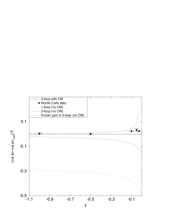
Figure 9: Perturbative results of the scalar condensate compared to Monte Carlo data. The straight line is the CW-optimized result, which has been substracted from the others.

The CW-method is in principle applicable even above the critical temperature and seems to produce reasonable results at $y$ values up to $y_{c}$. However, the CW-results are consistently below the Monte Carlo data. This discrepancy is small (typically less than 4%) but statistically meaningful. The systematic error of CW method is not sufficient to explain this effect, as can be seen from table 1, so the effect is probably due to higher order corrections.

Figure 10: Continuum limit of scalar mass at $y=-0.05$.

Figure 11: Continuum limit of vector mass at $y=-0.05$.

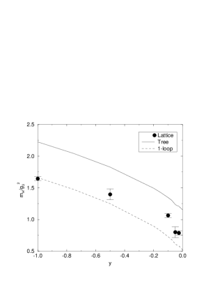
Figure 12: Perturbative results of scalar mass compared to Monte Carlo data.

4.4 Masses

The masses of scalar and vector particle at finite temperature were measured from the exponential decay of suitably chosen correlators. For scalar particle we used the operator

$$\phi^{\ast}(x)\phi(x),$$

and for vector

$$\mathop{\hbox{Im}}\phi^{\ast}(x)U_{i}(x)\phi(x+i).$$

The quality of our data for masses is not as good as the quality of the scalar condensate data, as can be seen from Figures 10 and 11, where we have plotted the results of the continuum extrapolation of both scalar and vector masses. However, the data is accurate enough to make some conclusions on the validity of perturbation theory.

The tree level calculation and the 1-loop values of scalar mass are plotted in Figure 12 with Monte Carlo data. The Monte Carlo data lies between tree and 1-loop values and is not consistent with either of them, implying that 1-loop calculation is probably not sufficient.

The Monte Carlo data for the vector mass is consistent with both 1-loop and tree values, as can be seen from Figure 13. However the statistical errors are so large that it is not possible to make definite conclusions on the validity of the perturbation theory.

The results obtained here are rather similar to those found in 3d SU(2)+ Higgs theory [14]. There it was found that the perturbative 1-loop calculation of vector mass agree extremely well with Monte Carlo data. To be able to confirm this result in U(1)+Higgs theory we would need to obtain more accurate Monte Carlo data for vector mass.

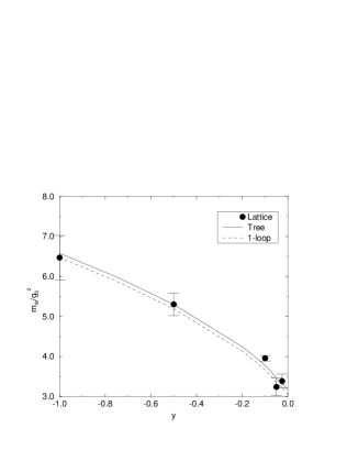
Figure 13: Perturbative results of vector mass compared to Monte Carlo data.

5 Conclusions

We have studied the validity of perturbation theory in the broken phase of the U(1)+Higgs theory. Firstly, by measuring the scalar condensate we examined the improvement of perturbation theory when increasing the number of loops and also the effect of the CW optimization procedure. Our results show that the 1-loop calculation is accurate only at $y$ values much lower than the critical value $y_{c}$. At $y=-1$, which is the smallest value of $y$ we examined, the error was already 13% and at largest value $y=-0.025$ the error was 73%. Even the 2-loop calculation is not accurate near $y_{c}$. The error was only 1% at $y=-1$, but 22% at $y=-0.025$. However, optimized perturbation theory provides accurate estimates at 2-loop level even up to the critical temperature. The largest error was 4% at $y=-0.05$. This indicates the importance of optimized 2-loop perturbative results.

The 1-loop perturbative calculation of the scalar mass shows deviations from Monte Carlo data. The average difference between perturbative and lattice results was 25%. We interpret this as a result of the insufficiency of a 1-loop perturbative calculation. This interpretation is supported by the fact that the 1-loop values of scalar condensate also show similar deviations. For the condensate 2-loop computations are available and their inclusion improves the situation considerably. For the scalar mass a 2-loop result is unfortunately available only for the pure scalar case [15]. It would be very interesting to have the 2-loop result for the scalar propagator also for gauge theories; then perturbation theory could be optimized and probably a much better agreement could be obtained.

The accuracy of our data for the vector mass has to improve before we can make any definite conclusions on the validity of perturbation theory for that quantity. One possibility would be to use the smearing or fuzzying technique [16], which has proven to be effective in SU(2)+Higgs theory [17] at sufficiently high or low temperatures.

Acknowledgements

The authors thank K. Kajantie for his support and encouragement on preparation of this paper. We also thank M. Laine for many discussions and comments and K. Rummukainen for his help on implementing the simulation program.

References

• [1] T. Banks and E. Rabinovici, Nucl. Phys. B 160 (1979) 349.
E. Fradkin and S. Shenker, Phys. Rev. D 19 (1979) 3682.
K. Jansen, J. JersΓ‘k, C.B. Lang, T. Neuhaus and G. Vones, Phys. Lett. B 155 (1985) 268; Nucl. Phys. B 265 (1986) 129.
H.G. Evertz, V. GrΓΆsch, K. Jansen, J. JersΓ‘k, H.A. Kastrup and T. Neuhaus, Nucl. Phys. B 285 (1987) 559.
H.G. Evertz, K. Jansen, J. JersΓ‘k, C.B. Lang and T. Neuhaus, Nucl. Phys. B 285 (1987) 590.
P.H. Damgaard and U.M. Heller, Phys. Rev. Lett. 60 (1988) 1246.
B. Krishnan, U.M. Heller, V.K. Mitryushkin and M. MΓΌller-Preussker, HU-BERLIN-IEP-96-16, hep-lat/9605043
• [2] K. Farakos, K. Kajantie, K. Rummukainen and M. Shaposhnikov, Nucl.Β Phys.Β B 425 (1994) 67.
• [3] K. Farakos, K. Kajantie, K. Rummukainen and M. Shaposhnikov, Nucl.Β Phys.Β B 442 (1995) 317.
• [4] C. Dasgupta and B. I. Halperin, Phys. Rev. Lett. 47 (1981) 1556.
J. Bartholomew, Phys. Rev. B 28 (1983) 5378.
W. BuchmΓΌller and O. Philipsen, Phys. Lett. B 354 (1995) 403.
A. JakovΓ‘c, A. PatkΓ³s and P. Petreczky, Phys. Lett. B 367 (1996) 283.
B. Bergerhoff, F. Freire, D. Litim, S. Lola and C. Wetterich, Phys. Rev. B 53 (1996) 5734.
• [5] K. Kajantie, M. Karjalainen, M. Laine and J. Peisa, in preparation.
• [6] P. Ginsparg, Nucl. Phys. B 170 (1980) 388.
T. Appelquist and R. Pisarski, Phys. Rev. D 23 (1981) 2305.
S. Nadkarni, Phys. Rev. D 27 (1983) 917.
• [7] K. Kajantie, M. Laine, K. Rummukainen and M. Shaposhnikov, Nucl. Phys. B 458 (1996) 90.
• [8] P. Arnold and O. Espinosa, Phys. Rev. D 47 (1993) 3546.
• [9] N. P. Landsman, Nucl. Phys. B 322 (1989) 498
• [10] M. Laine, Nucl. Phys. B 451 (1995) 484.
• [11] A. Hebecker, Z. Phys. C 60 (1993) 271.
• [12] T. Hattori and H. Nakajima, Nucl. Phys. B, Proc. Suppl. 26 (1992) 635.
• [13] Z. Fodor and K. Jansen, Phys. Lett. B 331 (1994) 119.
• [14] K. Kajantie, M. Laine, K. Rummukainen and M. Shaposhnikov, Nucl. Phys. B 466 (1996) 189.
• [15] A. Rajantie, HU-TFT-96-22, hep-ph/9606216.
• [16] B. Berg and A. Billoire, Phys. Lett. B 166, 203 (1986).
M. Teper, Phys. Lett. B 183, 345 (1986).
M. Albanese et al. Phys. Lett. B 192, 163 (1987).
A. S. Kronfeld, J. K. M. Moriarty and G. Schierholz, Comp. Phys. Comm. 52 (1988) 1.
• [17] O. Philipsen, M. Teper and H. Wittig, Nucl. Phys. B 469 (1996) 445.