Abstract. We study the interface between two different $Z(3)$ vacua in the deconfined phase of $SU(3)$ pure gauge theory in $2+1$ dimensions just above the critical temperature. In simulations of the Euclidean lattice gauge theory formulation of the system we measure the fluctuations of the interface as the critical temperature is approached and as a function of system size. We show that the intrinsic width of the interface remains small even very close to the critical temperature. Some dynamical exponents which govern the interaction of the interface with our Monte Carlo algorithm are also estimated. We conclude that the $Z(3)$ interface has properties broadly similar to those in many other comparable statistical mechanical systems.

1 Introduction

It has been known for some time that pure gauge theories have a non-confining high-temperature phase [1]and so any theory which is in a confining phase at zero temperature ($T=0$) must have a deconfining phase transition at some finite critical temperature, $T_{c}$. Pure non-abelian $SU(N)$ gauge theories, such as QCD without dynamical fermions, display this behaviour in both $2+1$ and $3+1$ dimensions. At low temperatures the colour charge of QCD is confined which is why no free quarks are seen in the relatively cool universe of today. At high temperatures, there is a non-confining phase, corresponding to the free quark-gluon plasma believed to exist in the hot early universe. In fact there are in general several degenerate phases of this type – as many as the number of elements of the centre, $Z(N)$, of the gauge group. Fermionic matter breaks the vacuum degeneracy, albeit on a small scale, so we consider only the pure gauge theory in what follows.

Two different types of interface are possible in the theory. The first is between the ordered and disordered phases and is only stable at the critical temperature where the two phases can coexist. Secondly, an interface can form between two of the ordered phases with different $Z(N)$ vacua, and this is usually called an “order-order interface”, or “$Z(N)$ interface”. Clearly, this type of interface can only exist above the critical temperature.

From the thermodynamic point of view there is something strange about these interfaces. On entropic grounds one expects to find disorder at high temperatures and order at low temperatures, not the other way round. The fundamentally Euclidean nature of this picture may be responsible [2, 3, 4]; there is no sensible counterpart to the Euclidean order parameter in Minkowski space (a naive Wick rotation leads to an imaginary time-like gauge field in Minkowski space) and so it may be that the interfaces do not exists as physical objects in the high temperature universe. Indeed, it has even been suggested [5] that only one true physical phase exists, even in Euclidean space, at high temperatures but recent numerical work does not support this point of view. Whether or not they are a Euclidean artifact, by virtue of their contribution to the partition function and to expectation values calculated using the Euclidean path integral, the interfaces must be included (like the instanton) in a non-perturbative analysis of the thermodynamics of QCD.

Recently the properties of $Z(N)$ interfaces at very high temperatures have been investigated numerically in $2+1$ dimensions [7, 8]. These simulations give a non-perturbative check on the conclusions of analytic calculations [9, 10] and show very good agreement; thus there is no reason to suppose that the $Z(N)$ phases are not distinct at high temperatures. In this paper we investigate the behaviour of the interface at much lower temperatures close to the critical temperature where it disappears. We shall be concerned not with the usual thermodynamical quantities, which have been thoroughly investigated [11], but rather with the geometrical properties and structure of the interface itself.

This paper is organised as follows. In section two we review briefly the theory of the deconfinement transition and the theoretical basis on which we shall analyse the simulation data on the interfaces. In section three we discuss the practical difficulties in identifying the interface from the gauge field configuration and describe how we have overcome them; some other aspects of the data analysis are also discussed. Section four contains the results that we have obtained characterising the interface fluctuations, and section five gives our results for various other properties of the interface. In section six, we give our conclusions and discuss some of the remaining puzzles associated with these interfaces.

2 Theoretical Background

In the Euclidean formalism, equilibrium finite-temperature field theory is obtained by considering a system which is of infinite volume but compact in the Euclidean time direction with period $\beta_{T}=T^{-1}$. In a lattice field theory implementation, it is of course not possible to vary the number of lattice spacings in the time direction, $L_{t}$, continuously; instead we work with a fixed $L_{t}$ and vary the gauge coupling, $\beta$, so that the lattice correlation length, and hence the physical value of the lattice spacing, $a$, and hence the physical $\beta_{T}=L_{t}a$, vary continuously.

The phases of a gauge theory at finite temperature are characterised by the free energies of static configurations of quarks and antiquarks [12]. The self-energy of a single quark in the gluon medium, $F_{q}$, is related to the expectation value, $L({\bf x})$, of a single Polyakov line, a time-ordered Wilson loop which wraps around the time boundary for a fixed spatial location ${\bf x}$,

$${L({\bf x})=\hbox{${1\over 3}$}{\rm Tr}{\cal T}e^{ig\int_{0}^{1/T}d\tau A_{0}(\tau,{\bf x})}=e^{-{\beta_{T}}F_{q}}.}$$ (1)

If $<L({\bf x})>=0$ then the insertion of a single quark will require infinite energy, corresponding to a confining phase. In contrast, if $<L({\bf x})>\neq 0$ then the insertion energy will be finite and isolated colour charges can exist – this is the deconfined phase. Thus, the expectation value of the Polyakov line gives an effective test for confinement.

A general non-Abelian gauge transformation which leaves the Euclidean QCD action, ${\cal S}_{E}$, invariant will also leave $L$ invariant if the transformation is periodic in time. However, ${\cal S}_{E}$ is actually invariant under an additional global symmetry. In the lattice formulation this consists of multiplying each time-like link variable at a given time slice by an element of the centre of the gauge group (the set of elements which commute with all members of the group, $Z(N)$ in the case of $SU(N)$). This global symmetry is an invariance of ${\cal S}_{E}$ and cannot be undone by a gauge transformation. The topologically non-trivial Polyakov line, which wraps around the periodic boundary condition in the time direction, is not invariant under these transformations, but is rotated by an element, $z$, of the centre: $L({\bf x})\rightarrow zL({\bf x}).$ Clearly, $<L({\bf x})>$ acts as an order parameter for the centre symmetry, distinguishing between broken and unbroken phases, and between the different broken phases [9, 13].

In the deconfined phase, where the $Z(N)$ symmetry has been spontaneously broken, the system can exist in any one of $N$ degenerate vacua. It is possible to arrange boundary conditions of the system so that different parts of it exist in different vacua, i.e. different $Z(N)$ phases. The existence of these distinct domains forces the appearance of domain walls, or “$Z(N)$ interfaces”, where they meet [9, 10]. Within these interfaces, the gauge fields interpolate between the different vacua, as does the expectation value of the Polyakov line. A perturbative calculation at large $\beta$ [9] leads to the conclusion that an instanton interpolating between two vacua should have characteristic size, $l_{W}$ of order $1/g\sqrt{T}$; therefore, at least at large enough $\beta$, we expect the interface to have an intrinsic width of this magnitude as well. This length scale is the same order as the Debye screening length, $l_{D}$ which governs gauge-invariant correlation functions of the time-like component of the gluon field ($A_{0}$) at large distances and high temperatures. The free energy of a quark-antiquark pair, over and above the sum of their separate free energies, vanishes as the quarks become infinitely far apart, and, from perturbation theory, we know that quarks are screened at a distance of the order of the inverse electric mass, so rather than being logarithmic in ${\bf x}$, the interaction potential takes the form

$$F_{q\overline{q}}({\bf x})-2F_{q}=V(|{\bf x}|,T)\mathrel{\mathop{\sim}\limits_{|{\bf x}|\rightarrow\infty}}-C\exp\left(-2{|{\bf x}|\over l_{D}}\right)\qquad\hbox{for\ }T>T_{c}.$$ (2)

The factor of two arises because gauge invariance leads to an exchange of two gluons being the lowest-order contribution in perturbation theory. The Debye screening length is known [14] to have logarithmic corrections so that

$$l_{D}={1\over g\sqrt{T}}.{1\over{3\over 4\pi}\log({\beta\over 12})+\ldots}$$ (3)

The corresponding corrections to $l_{W}$ have not been calculated so, even at very high temperature, a direct comparison between the interface width and the Debye screening length is not possible. At low temperatures, near the critical point, we expect all these quantities to be functions of $\beta-\beta_{c}$ and there are no analytic results available with which to compare our simulations.

At very high temperatures the magnitude of $<L>$ is large; the change in its argument from one $Z(N)$ phase to the other is abrupt. The interface between the two phases is sharp (see fig. 2 of section 3); it is essentially a one-dimensional object that separates the phases and exhibits relatively small transverse fluctuations. As $\beta$ decreases towards its critical value, $<L>$ vanishes according to

$$<L>\sim(\beta-\beta_{c})^{\beta_{M}},$$ (4)

where $\beta_{c}=8.175(2)$ in the infinite spatial volume limit on $N_{t}=2$ lattices, and the measured critical exponent $\beta_{M}$ [15, 11] is consistent with the universality prediction of ${1\over 9}$ from the three-state Potts model [16]. However, this only tells us about the expected height of the interface and not about its geometrical nature as $\beta$ decreases (except that it must ultimately disappear at $\beta_{c}$). It may be that, as the free energy per unit length declines, the interface undergoes increasingly violent fluctuations while remaining intrinsically a one-dimensional object, the height of the interface declining until it vanishes at $\beta_{c}$. An alternative is that the interface may become intrinsically broader, thus becoming more two-dimensional, with more and more regions of disordered phase within it. At $\beta_{c}$ these disordered regions expand to take over the whole system and the interface disappears.

Figure 1: The vacuum diagrams corresponding to the 2nd, 4th and 6th connected vacuum correlation functions respectively. The open circle simply denotes point ${\bf x}$, the endpoint of each external leg; the solid circle denotes an interaction vertex, $\lambda$; and the momentum travelling along a leg is denoted by $k$.

To help in the analysis of the fluctuations of the interface we shall compare them to a simple model. Our lattice is taken to have $L_{x}\sim 3L_{y}\gg\L_{t}$ ; the boundary conditions are periodic and a “twist” is introduced (after [17]) to ensure that for $x\sim 0$ the system is in one $Z(3)$ phase while for $x\sim L_{x}$ it is in a different one. The interface thus forms stretching across the lattice in the $y$ direction and separating the two phases. Now let $\phi(y)$ denote the displacement, in the $x$ direction, of the interface from its equilibrium position and construct a simple effective Lagrangian, $\cal L$, for $\phi$. Translational invariance dictates that $\cal L$ can only depend on $\partial_{y}\phi$ and invariance under $\phi\to-\phi$ rules out odd powers; if the interface were just executing a free random walk across the lattice then ${\cal L}\sim(\partial_{y}\phi)^{2}$. To obtain non-gaussian moments a correction term must be added and the simplest resulting Lagrangian is

$${\cal L}={1\over 2}\gamma(\partial_{y}\phi)^{2}+{\lambda\over 4!}(\partial_{y}\phi)^{4}$$ (5)

which fits the data quite well with

$$\gamma \sim (\beta-\beta_{c})^{\nu_{1}}$$

$$\lambda = \ell\lambda_{0}$$

$$\lambda_{0} \sim (\beta-\beta_{c})^{\nu_{2}}$$ (6)

where the length scale $\ell$ appears in $\lambda$ on dimensional grounds. It can be any combination of the two length scales which may be relevant, $L_{y}$ and $l_{D}$. The diagrams for the first three even moments of $\phi$ are shown in fig.1. It is straightforward to compute the connected correlation functions from $\cal L$ although the mode sums have to be done numerically. Putting $\ell=L_{y}$ the connected correlation functions (denoted by $<.>_{c}$) are then predicted to behave like

$$<\phi^{2}> \sim L_{y}\gamma^{-1}$$

$$<\phi^{4}>_{c} \sim L_{y}^{2}\gamma^{-4}\lambda_{0}$$

$$<\phi^{6}>_{c} \sim L_{y}^{3}\gamma^{-7}\lambda_{0}^{2}$$ (7)

3 Identifying the Interface

Fig.2 shows the $Z(3)$ interface on a particular gauge field configuration for a number of $\beta$ values. As discussed in section 2, at high $\beta$ the interface is sharp and well defined; however by $\beta=9$, still some way above the critical value, it is becoming difficult to identify the location of the interface by eye with any degree of certainty.

Figure 2: Polyakov line (real part) profiles of the same $Z(3)$ interface at different temperatures. The top left picture shows the interface on a $2\times 24\times 96$ lattice with $\beta=50$. Going from left to right, and then top to bottom, the other pictures illustrate an interface between the same phases ($<L>\approx e^{2\pi i/3}$ on the left and the $<L>\approx 1$ on the right) for $\beta=10,9,8.5,8.3$ and $8.1$ respectively.

One way to deal with the increase in phase fluctuations is to cut out the highest frequency modes altogether. This can be achieved most simply by a “box-car” average, where the Polyakov lines of each three-by-three spatial array of points are averaged over to give a new value, allocated to the central point. The effect of smoothing out the fluctuations is shown in fig.3, produced by applying the box-car average to the pictures of fig.2. To make things even clearer, the Polyakov lines have first been re-binned so that the $24\times 96$ spatial dimensions become $12\times 48$, with each two-by-two array being averaged to one point. Now the $Z(3)$ interface can clearly be seen for all but the last picture, i.e. for all temperatures above $\beta_{c}$. The fact that the interface can still be seen for temperatures just above the critical value suggests that a study of its structure should still be possible quite close to the phase transition.

Figure 3: Smoothed Polyakov line profiles, produced by processing the raw pictures of fig.2. As in that figure, $\beta=50,10,9,8.5,8.3$ and $8.1$ respectively.

However, there is a drawback with this smoothing technique as it averages out a whole class of fluctuations which may be important in the interface collapse. A more satisfactory method is to produce a contour map from the real part of the Polyakov lines on the lattice. Consider following a contour whose height is mid-way between that of the average Polyakov line at the low-$x$ end of the lattice and that at the high-$x$ end. This picks out the mid-height of the interface as it goes across the lattice, as well as any bubbles of fluctuating phase which are large enough to cross the contour height. The crucial point to note is that only the $Z(3)$ interface will cross the entire lattice, i.e. the only contour that will wrap once around the lattice in the transverse ($y$) direction is that corresponding to the interface. Any contour representing a bubble of phase will join up with itself without a net crossing of any lattice boundary. This enables us to tell the interface apart from any fluctuations, and to identify the position of its mid-height. By following contours at various heights between the two extremes, we can study more of the structure of the interface. The advantage of using contours is that no prior processing of the Polyakov line data is required. We can also study contours of the box-car-averaged data and this can be useful very close to the critical temperature.

Figure 4: Options for the contour-following algorithm. Given a point at the desired contour level on the lower side, the Polyakov lines at the upper two corners determine the progress of the contour in cases (i)-(iii). A plus (minus) sign indicates a Polyakov line value greater (less) than the contour level. The same corner configurations of (iv) and (v) give two possible contour directions; we choose between them by considering the central average of the corner values. These pictures exhaust all possibilities for the values of the lower corners given, but any general configuration can be rotated and reflected into one of these.

To find a contour at a particular level, we return to the raw Polyakov line data. For $y=0$, the algorithm follows a procedure similar to that above: starting from the centre, $x=L_{x}/2$, it looks for the nearest point passing through the contour level. Then, it considers the square of points formed by the two neighbouring lattice sites at $y=0$ and the corresponding sites at $y=1$. The algorithm decides to which side of the square the contour should go, as detailed in fig.4. Then, starting with this side, the whole procedure continues. Eventually, the contour must join up with itself. Repeated application of this technique for different contour levels determines the structure of the interface to the desired precision. The same procedure can be applied to the smoothed Polyakov line configurations, to obtain smoothed contour maps.

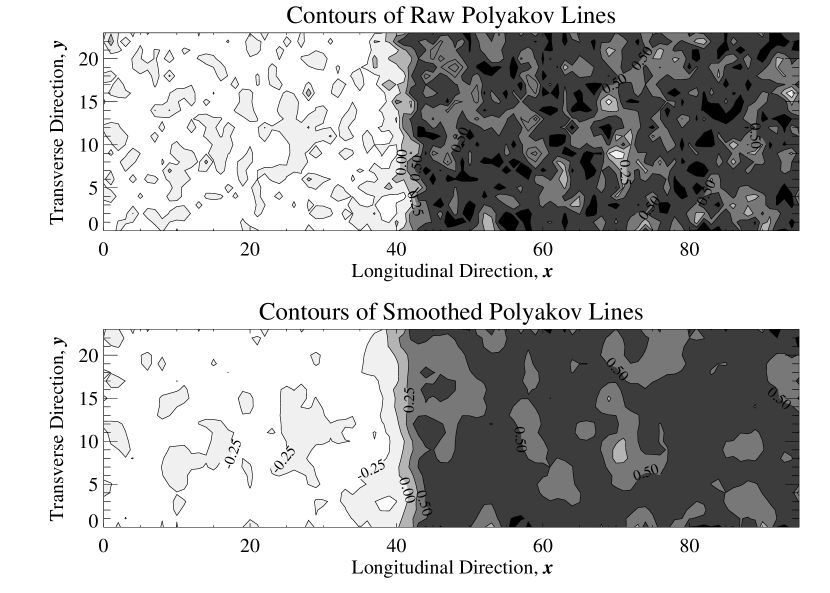
Figure 5: Contour maps of raw and processed Polyakov lines for $\beta=10$ on a $2\times 24\times 96$ lattice. These maps correspond to the $\beta=10$ pictures of fig.2 and fig.3 respectively. The contour levels are at $-0.25,0,0.25,0.5$ and $0.75$, darker regions corresponding to higher values.

An example of a contour map is shown in fig.5, for the same $\beta=10$ gauge configuration featured in fig. 2 and fig. 3. Note that the interface in the centre of the maps is represented by the only contours going all the way across the lattice. The first picture shows the raw data of fig.2; the second, the smoothed data of fig.3.

Left to its own devices, the interface will execute a random walk in the $x$ direction. When the interface reaches $x\sim 0$ or $x\sim L_{x}$ it will interact with the twist and tunnel into different $Z(3)$ vacua, producing a different $Z(3)$ interface each time. However to study the profile of one particular $Z(3)$ interface without interference from other vacua the interface should be held in place well away from the twist, so that no part of it, even its wildest fluctuation, passes through the twist. After each Monte-Carlo (MC) sweep of the lattice, we locate the position of the interface, and then slide the whole gauge configuration along the lattice until the interface is re-centred at $x\approx L_{x}/2$. Any link variables which are shifted through the twist are multiplied by the appropriate factor, so there is no physical effect and no violation of translation invariance arising from this procedure.

For our MC simulations, we used a mix of Cabibbo-Marinari heat-bath steps [18], using the Kennedy-Pendleton algorithm [19] to update $SU(2)$ subgroups, and Brown-Woch over-relaxation steps [20], after using many initial heat-bath sweeps to equilibrate the system. Measurements of physical operators took place only every four sweeps, to reduce the correlations caused by adjacent configurations. Since we were interested in the evolution of the interface, contour measurements were taken after every sweep of the lattice. In order to study finite-length effects for the interface, we performed simulations on a number of different lattice widths ($L_{y}=18,24,30,36,42,48,54$) and length $L_{x}=72$, chosen after studies with various lengths to ensure that not even the wildest fluctuations of the interface would reach as far as the twist during our full-length runs. We used $\beta$ values of 8.25, 8.35, 8.50, 8.75 and 9.00 to study the behaviour of the interface close to $\beta_{c}$. The simulations consisted, in each case, of 2k heat-bath sweeps and 100k main sweeps. Approximately 100—200 hours of CPU time on a DEC 2100 A500MP machine were needed for each value of $\beta$.

The statistical analysis of our data, and especially of the Wick-subtracted moments which are not expected to be normally distributed, is quite complicated and requires a method which does not rely on a priori knowledge of their distribution. We used methods based on the bootstrap principle [21] and full details are given in [22].

4 The Fluctuation Moments of the Interface

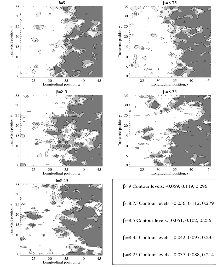
Figure 6: Contour maps of the interface on a $2\times 36\times 72$ lattice, for decreasing temperature. Moving left to right, and then top to bottom, the picture illustrates the interface structure around the longitudinal centre of the lattice after 2k heat-bath and 60k main sweeps for $\beta=9,8.75,8.5,8.35$ and $8.25$.

In fig.6, a contour snapshot of the interface is shown for each temperature studied, at the same point in each simulation, just over halfway through. Three contours have been followed in each case. We can see that the contours stay close together across most of the interface, indicating that the interface remains relatively narrow as the temperature drops. The shape of the interface appears to fluctuate rather more wildly with the falling temperature, but the interface does not spread out noticeably in width.

As discussed in section 2, the fluctuations are characterised by their moments $<\phi(y)^{n}>_{c}$; $\phi(y)$ can be the displacement from its mean position of any contour that has been identified. We measured the first six moments, and took separate sets of data for each of the three contours followed, at 25%, 50% and 75% of the height of the interface respectively. The qualitative behaviour is roughly the same for each contour. The upper and lower contours are subject to rather more fluctuation than the middle one, as we expect since they are closer to the outside of the interface and therefore more susceptible to bubbles of phase forming nearby and distorting the edge of the interface. The even moments behave very smoothly, whilst the odd moments are very much smaller and show more variation; the first moment must average to zero by definition, and we expect all odd moments to tend to zero for infinite statistics. We also computed the behaviour of the moments of smoothed data and found that it is very similar to that of the raw data, both qualitatively and quantitatively. This indicates that the smoothing procedure does not lose a significant amount of information about the fluctuations and is consistent with the notion that the important fluctuations take place on a distance scale much larger than the lattice spacing.

Our results for $\beta\geq 8.35$ show reasonable statistical distributions for the moments over the 100k sweeps. However, those for $\beta=8.25$ and smaller $L_{y}$ occasionally contain “spikes”, observations for the moments which are far larger than we would expect, sometimes by several magnitudes. The spikes are not caused by wild fluctuations passing through the twist, since similar spikes are not seen for the widest lattices where fluctuations are larger. They are an artefact of the greater energetic instability of the smaller interfaces near the critical point. If parts of the interface collapse during interaction with nearby bubbles of phase, the interface contour may briefly undergo a drastic distortion or partial collapse, even appearing to pass through the twist because of the change in Polyakov values there and confusing our algorithm. We cannot prevent the spikes occurring, since the cause is a real physical process, but they can have a serious effect on the overall averages, especially for the higher moments. Thus, we would like to be able to examine the data with the spikes removed. To do this, we impose an upper cut-off on the statistical distributions. To ensure that only the spikes are removed, we need to define the cut-off in a statistically sensible manner. We take it, for each distribution, to be the median plus 2.5 times the interquartile range of the distribution of logarithmic values of data, where the interquartile range is defined to run between the 25th and 75th percentiles of the distribution. This ensures that the cut-off corresponds only to the upper tip (to be precise, the top 0.04%) of a normal distribution, ensuring that only data sets containing spikes are affected by the procedure. The exact multiplier “2.5” can, of course, be varied, but we find that a lower number (e.g. 2.0, cutting off 0.3% of the distribution), has too great an effect on the normal contribution to the distributions, whereas a higher number (e.g. 3.0, cutting off only 0.002% of the normal distribution) permits too much influence from the spikes. The procedure is fully detailed in [22]. In our tabulated results values which were obtained with this procedure in effect are marked with a †.

     Table 1: Estimates of $<\phi^{2}>$ from Raw Data (Corrected), 50% Contour                       $\beta\ddots L_{y}$ 18 24 30 36 42 48 54 Slope                                         8.25 $5.44^{+0.05}_{-0.04}$ $8.09^{+0.06}_{-0.06}$ $11.9^{+0.1}_{-0.1}$ $14.3^{+0.1}_{-0.1}$ $17.8^{+0.1}_{-0.1}$ $20.8^{+0.2}_{-0.2}$ $23.1^{+0.2}_{-0.2}$ _1.33±0.02                                         8.35 $4.52^{+0.03}_{-0.03}$ $6.69^{+0.05}_{-0.05}$ $9.13^{+0.07}_{-0.06}$ $11.4^{+0.1}_{-0.1}$ $13.4^{+0.1}_{-0.1}$ $16.5^{+0.1}_{-0.1}$ $18.2^{+0.1}_{-0.1}$ _1.27±0.01                                         8.50 $3.93^{+0.03}_{-0.03}$ $5.19^{+0.03}_{-0.03}$ $7.17^{+0.05}_{-0.05}$ $8.89^{+0.07}_{-0.06}$ $10.0^{+0.1}_{-0.1}$ $11.9^{+0.1}_{-0.1}$ $13.8^{+0.1}_{-0.1}$ _1.15±0.01                                         8.75 $3.06^{+0.02}_{-0.02}$ $4.21^{+0.03}_{-0.03}$ $5.32^{+0.04}_{-0.03}$ $6.34^{+0.04}_{-0.04}$ $7.62^{+0.05}_{-0.05}$ $8.85^{+0.06}_{-0.06}$ $9.57^{+0.06}_{-0.06}$ _1.05±0.01                                         9.00 $2.62^{+0.02}_{-0.02}$ $3.44^{+0.02}_{-0.02}$ $4.38^{+0.03}_{-0.03}$ $5.27^{+0.03}_{-0.03}$ $6.29^{+0.04}_{-0.04}$ $7.37^{+0.05}_{-0.05}$ $7.89^{+0.05}_{-0.05}$ _1.03±0.01                                         Slope _{-0.31±0.03 -0.36±0.03 -0.42±0.03 -0.42±0.03 -0.44±0.02 -0.45±0.03 -0.46±0.04}                       

     Table 2: Estimates of $<\phi^{4}>_{C}$ from Raw Data (Corrected), 50% Contour                       $\beta\ddots L_{y}$ 18 24 30 36 42 48 54 Slope                                         8.25 $63.2^{+3.7}_{-3.0}$ $115^{+7}_{-5}$ $273^{+14}_{-11}$ $326^{+9}_{-9}$ $425^{+15}_{-14}$ $580^{+14}_{-13}$ $658^{+15}_{-15}$ _2.12±0.07                                         8.35 $30.6^{+1.0}_{-1.1}$ $61.7^{+2.1}_{-2.0}$ $108^{+3}_{-3}$ $166^{+6}_{-5}$ $197^{+6}_{-6}$ $322^{+1}_{-1}$ $299^{+10}_{-9}$ _2.17±0.06                                         8.50 $19.2^{+0.6}_{-0.5}$ $27.8^{+0.8}_{-0.8}$ $59.0^{+2.0}_{-1.8}$ $82.0^{+2.8}_{-2.5}$ $87.8^{+2.8}_{-2.8}$ $126^{+5}_{-4}$ $163^{+6}_{-5}$ _1.97±0.05                                         8.75 $9.68^{+0.34}_{-0.31}$ $16.3^{+0.6}_{-0.6}$ $22.3^{+0.7}_{-0.6}$ $30.3^{+1.1}_{-1.0}$ $43.0^{+2.2}_{-2.0}$ $48.2^{+1.9}_{-1.7}$ $49.7^{+1.9}_{-1.8}$ _1.55±0.04                                         9.00 $5.84^{+0.17}_{-0.16}$ $8.76^{+0.25}_{-0.25}$ $13.0^{+0.4}_{-0.4}$ $15.6^{+0.6}_{-0.5}$ $23.3^{+0.8}_{-0.8}$ $28.6^{+1.1}_{-1.0}$ $28.5^{+1.3}_{-1.0}$ _1.54±0.03                                         Slope _{-0.99±0.06 -1.10±0.07 -1.28±0.07 -1.25±0.11 -1.21±0.06 -1.27±0.11 -1.28±0.12}                       

     Table 3: Estimates of $<\phi^{6}>_{C}$ from Raw Data (Corrected), 50% Contour                       $\beta\ddots L_{y}$ 18 24 30 36 42 48 54 Slope                                         8.25 $3530$ $6330$ $23500$ $18500$ $18500$ $14500$ $15200$ _1.46±0.22 ${}^{+490}_{-400}$ ${}^{+1080}_{-990}$ ${}^{+3500}_{-2800}$ ${}^{+1600}_{-1500}$ ${}^{+3400}_{-2600}$ ${}^{+2800}_{-2300}$ ${}^{+3400}_{-2900}$                                         8.35 $712$ $1700$ $2860$ $5180$ $4790$ $10200$ $2640$ _2.38±0.29 ${}^{+75}_{-55}$ ${}^{+210}_{-190}$ ${}^{+440}_{-390}$ ${}^{+670}_{-580}$ ${}^{+1050}_{-840}$ ${}^{+2100}_{-1700}$ ${}^{+2300}_{-1680}$                                         8.50 $259^{+29}_{-23}$ $350^{+85}_{-73}$ $1090^{+160}_{-150}$ $1710^{+350}_{-280}$ $912^{+316}_{-250}$ $1580^{+430}_{-360}$ $1020^{+670}_{-510}$ _1.84±0.22                                         8.75 $82.5^{+9.9}_{-8.6}$ $142^{+40}_{-35}$ $102^{+30}_{-24}$ $61.5^{+46.0}_{-43.4}$ $244^{+116}_{-102}$ $17.3^{+101.8}_{-78.0}$ $-634^{+111}_{-91}$ _?±?                                         9.00 $24.7^{+3.6}_{-3.1}$ $34.4^{+9.1}_{-9.5}$ $27.3^{+15.8}_{-13.9}$ $-35.7^{+19.5}_{-16.2}$ $-65.2^{+34.2}_{-28.0}$ $-214^{+47}_{-39}$ $-139^{+61}_{-47}$ _0.49±0.11                                         Slope _{-1.98±0.11 -2.10±0.15 -2.58±0.25 -1.94±0.60 -2.09±0.12 -2.79±0.80 -1.87±0.07}                       

Figure 7: The connected moments at $\beta=8.5$ plotted against the lattice width. Diamonds and boxes represent raw and smoothed data respectively. The lines are best fits to (8).

Fig.7 shows the dependence of the moments, calculated for both the raw and the smoothed 50% contour, on the lattice width at $\beta=8.5$. The slopes for the second and fourth moments are in reasonable agreement with the simple model results (7) although the agreement is not good for the sixth.

Figure 8: The connected moments with spike suppression at $\beta=8.5$.

In fig.8 we show the same data but with spike suppression in operation. The results are very similar to those shown in fig.7 demonstrating that the spikes are not a significant problem at $\beta=8.5$. The roughness exponents defined by

$$<\phi^{n}>_{c}\sim L_{y}^{n\alpha_{n}}$$ (8)

are tabulated in table 4 for all the $\beta$ values we have studied (an asterisk means that no statistically significant determination was possible).

Table 4

$\beta$	$2\alpha_{2}$	$4\alpha_{4}$	$6\alpha_{6}$
8.25	1.33(2)†	2.12(7)†	1.46(22)†
8.35	1.27(1)†	2.17(6)†	2.38(29)†
8.5	1.15(1)	1.95(5)	1.82(26)
8.75	1.05(1)	1.54(4)	*
9.0	1.03(1)	1.54(3)	*

Figure 9: The connected moments on the $L_{y}=36$ lattice plotted against $\beta$. The lines are best fits to (9).

In fig.9, we plot the moments at fixed $L_{y}=36$ against $\beta$ when the spike-suppression procedure discussed above is not operating. The lines are fits of the form

$$<\phi^{n}>_{c}\sim(\beta-\beta_{c})^{-\gamma_{n}}$$ (9)

taking $\beta_{c}=8.175$. Comparing the second and fourth moments with (7) we find that

$$\gamma\sim(\beta-\beta_{c})^{0.43(3)},\qquad\lambda_{0}\sim(\beta-\beta_{c})^{0.25(14)}$$ (10)

which then predict that

$$<\phi^{6}>_{c}\sim(\beta-\beta_{c})^{-2.51(21)},$$ (11)

within roughly one standard deviation of the observed behaviour.

Figure 10: The connected moments with spike suppression on the $L_{y}=36$ lattice plotted against $\beta$. The lines are best fits to (9).

In fig.10 we show the same data as for fig.9 but with spike suppression. We see that the results for the second moment are scarcely affected and the change for the fourth moment is fairly small but the effect on the sixth moment, which we would expect to be most affected by the spikes, is substantial.

Table 5

$L_{y}$	$\gamma_{2}$	$\gamma_{4}$	$\gamma_{6}$
18	.41(1)	.99(6)†	1.98(11)†
24	.37(2)	1.10(7)†	2.10(15)†
30	.44(2)	1.28(7)†	2.58(25)†
36	.43(3)	1.25(11)†	1.96(60)†
42	.44(2)	1.29(5)	2.09(12)†
48	.45(3)	1.26(12)	2.79(80)†
54	.46(4)	1.32(11)	1.87(57)†

Again comparing the second and fourth moments with (7) we find that

$$\gamma\sim(\beta-\beta_{c})^{0.42(3)},\qquad\lambda\sim(\beta-\beta_{c})^{0.43(16)}.$$ (12)

which in turn predict that

$$<\phi^{6}>_{C}\sim(\beta-\beta_{c})^{-2.08(24)},$$ (13)

extremely close to the observed behaviour. The other sets of revised data now give very consistent results for $\gamma$ and $\lambda$.

Our other sets of data give similar results and the $\gamma_{n}$ are tabulated in table 5 for all the $L_{y}$ values we have studied.

5 The Interface Width, Screening and Mobility

Figure 11: The transverse Polyakov lines at $\beta=9.0$ and the weighted first differences discussed in the text.

We define the transverse averaged Polyakov line by

$$\overline{L}(x,L_{y})=L_{y}^{-1}\sum_{y}L(x,y)$$ (14)

At very high temperatures where the interface is essentially rigid we expect it to show the classic instanton shape and be independent of $L_{y}$ [9]

$$\overline{L}(x,L_{y})=f(x)\sim A\tanh\left({x-x_{0}\over l}\right)+B$$ (15)

where $A$ and $B$ are constants and $l$ is the characteristic width of the interface. As the temperature decreases and the interface fluctuates more (roughens) some of the spread in $\overline{L}(x)$ will be caused by the roughening; provided the fluctuations are not too great, and assuming that the moments of $\phi$ are given by the free random walk results (good enough at the accuracy of measurement that we have), we can approximate the measured $\overline{L}(x,L_{y})$ by

$$\overline{L}(x,L_{y}) = L_{y}^{-1}\sum_{y}<f(x-\phi(y))>_{\phi}$$ (16)

$$= f(x)+L_{y}f_{1}(x)+L_{y}^{2}f_{2}(x)+\ldots$$

Figure 12: The interface width deduced from transverse Polyakov lines plotted against $\beta$.

The piece linear in $L_{y}$ can be removed by taking weighted first differences of measurements at different $L_{y}$,

$$\Delta\overline{L}(L_{1},L_{2}) = {L_{2}\overline{L}(x,L_{1})-L_{1}\overline{L}(x,L_{2})\over L_{2}-L_{1}}$$ (17)

$$= f(x)+O(L_{1,2}^{2})$$

In the same way both linear and quadratic $L_{y}$ dependence can be removed by taking weighted second differences. Fig.11 shows the results of this procedure at $\beta=9.0$; once the part linear in $L_{y}$ is removed all the curves collapse quite convincingly onto one. Fitting (15) to this universal curve a value for $l$ can be extracted. As $\beta$ is decreased the procedure, which essentially treats the fluctuations as a perturbation, works less well but the behaviour is reasonable down to $\beta=8.35$; it was not possible to measure $l$ at $\beta=8.25$. The results for $l$ are plotted in fig.12 and show a mild increase as $\beta$ decreases but we do not have enough information to extract any critical behaviour.

Figure 13: The average interface width, defined as twice the average separation of the 25% and 50% contours, measured in units of the lattice spacing.

We have also measured the interface width by using the contour data directly. The results of defining the width as twice the separation between 25% and 50% are shown in fig.13. Unfortunately we are only able to measure the separation in the $x$ direction; as the interface fluctuates this quantity is bound to be greater than the shortest distance between the contours and so it is inevitable that, especially at the smaller $\beta$ values, it will be over-estimated. Even without taking this into account we see that the width does not grow rapidly as the temperature decreases towards its critical value and the two methods for measuring the interface width yield qualitatively consistent results.

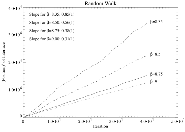
Figure 14: The wandering of the interface, for temperatures near the critical temperature, over 40k sweeps after an initial 400 heat-bath sweeps.

Figure 15: The divergence of the speed of the random walk in fig.12 as the temperature approaches its critical value.

Finally, as a curiosity, we have examined some quantities which describe the dynamical (in computer time) behaviour of the interface and therefore relate to the efficiency of our MC algorithm in equilibrating the interface itself. The speed of the random walk in the $x$-direction made by the interface can be measured by turning off the mechanism that constantly re-centres the interface. As the temperature drops and more and larger bubbles of the “wrong” phase form within the main domains, the interface will sometimes combine with them and so we might expect it to move faster. In fig.14, we do indeed see an increase in speed as the temperature drops and the speed appears to diverge as $\beta\rightarrow\beta_{c}$. This is shown more clearly in fig.15 where we fit the speed to a function of the form

$${{\partial x^{2}}\over{\partial t}}\sim(\beta-\beta_{c})^{\beta_{RW}}.$$ (18)

Our results suggest values of

$$\beta_{c}=8.14(3),\qquad\beta_{RW}=-0.71(6).$$ (19)

This value for $\beta_{c}$ is consistent with that obtained by other methods, and the dynamical exponent governing the critical acceleration of the random walk is given by $\beta_{RW}$.

Studies of discrete models [23] and continuum growth equations [24] in condensed matter systems make predictions for the behaviour of the width of an interface, usually defined to be the square-root of our second moment,

$$W(L_{y},t)=\sqrt{\overline{\phi^{2}}-{\overline{\phi}}^{2}},$$ (20)

as a function of the time, $t$, since its formation with initial width zero. For times much smaller than some critical time, $t_{X}(L_{y})$, determined by the interface size, an exponent $\beta_{G}$ will govern the growth of the width

$$W(t)\sim t^{\beta_{G}},\qquad t\ll t_{X}(L_{y}).$$ (21)

For times much larger than this the width is governed by $\alpha_{2}$, the roughness exponent, as we discussed in section 5. Fig.16 shows an example of the growth of a $Z(3)$ interface. At high $t$ the size saturates as usual, but at low $t$ we see growth governed by an exponent, as in the condensed matter models. For our interface, the average profile yields

$$\beta_{G}=0.61(2).$$ (22)

Figure 16: An example of the growth in size of an interface for $\beta=8.5,L_{y}=36$, and a growth profile averaged over all $L_{y}$ and $\beta$. In each case, $\beta_{G}$ is estimated from the slope of the dotted line.

6 Conclusions

Despite the increasing fluctuations and decreasing height of the interface as the critical temperature is approached we have shown that it is quite practicable to isolate it and to measure its geometrical properties. As one might expect of a second order transition the fluctuation moments diverge as $\beta\downarrow\beta_{c}$ in a manner which is to a good approximation independent of the transverse size of the lattice, $L_{y}$. That the relation between the three moments measured is more or less as predicted by the simple model (7) may be fortuitous because the model does not describe the dependence of the moments on the transverse size very well. One of the reasons why we are able to measure the fluctuations reliably is that the intrinsic width remains small; from the measurements we have made there is no real indication that this quantity does not remain finite as $\beta\downarrow\beta_{c}$. The dynamical (in computer time) behaviour of the interface is consistent with the usual behaviour encountered in other systems.

From this work and [7, 8] it seems clear that the $Z(N)$ interface in the Euclidean formulation of the theory really does have all the properties expected of such an interface in an ordinary statistical mechanical system as well as being consistent with weak coupling perturbation theory. The only objection to such a conclusion is that most of this work has been done at $L_{t}=2$. However the behaviour of the interface free energy in $SU(2)$ at high temperatures has been studied in [7] for $L_{t}=2,3,4$, and $6$ and they find essentially no $L_{t}$ dependence.

The relation of this picture to Minkowski space is as yet unclear. In the Euclidean path integral, the different $Z(N)$ vacua, and consequently domain walls between them, will appear in the ensemble of gauge field configurations that is integrated over to yield expectation values. We expect at least some observable quantities, call them $Q$, to depend upon the presence of these vacua in the sense that if there were only one vacuum $Q$ would be different. The observables must be the same when calculated in Minkowski space as in Euclidean space. It follows that there must be some (necessarily non-perturbative) feature of the ensemble of gauge field configurations in Minkowski space which is responsible for $Q$ taking a different value from the single Euclidean vacuum prediction (or else there are no $Q$s). The $Q$ observables potentially correspond to interesting physical effects such as baryogenesis and CP violation in the early universe [25, 26]; these calculations can be criticised on the grounds that they assume the Euclidean domain structure carries over to Minkowski space but it may be that the calculation can be reformulated entirely in Euclidean space in which case the results should be unambiguous.

We acknowledge valuable discussions with C.P. Korthals Altes and M. Teper. This work was supported by PPARC grants GR/J21354 and GR/K55752, and S.T.W. acknowledges the award of a PPARC studentship.

References

- [1] A. Polyakov, Phys. Lett. B72 (1978) 477.
- [2] V.M. Belyaev, I.I. Kogan, G.W. Semenoff and N. Weiss, Phys. Lett. B277 (1992) 331.
- [3] N. Weiss, UBCTP93-23 (hep-ph/9311233).
- [4] I.I. Kogan, Phys. Rev. D49 (1994) 6799.
- [5] A. V. Smilga, Ann. Phys. 234 (1994) 1.
- [6] A. Roberge and N. Weiss, Nucl. Phys. B275 (1986) 734.
- [7] C. P. Korthals Altes, A. Michels, M. Stephanov and M. Teper, OUTP-96-10P.
- [8] S. T. West and J. F. Wheater, Oxford University preprint OUTP-96-21P, hep-lat 9605040, to be published in Phys. Lett. B.
- [9] T. Bhattacharya, A. Gocksch, C. P. Korthals Altes and R. D. Pisarski, Nucl. Phys. B383 (1992) 497.
- [10] T. Bhattacharya, A. Gocksch, C. P Korthals Altes and R. D. Pisarski, Phys. Rev. Lett. 66 (1991) 998.
- [11] J. Christensen, G. Thorleifsson, P. H. Damgaard and J. F. Wheater, Nucl. Phys. B374 (1992) 225.
- [12] L. D. McLerran and B. Svetitsky, Phys. Rev. D24 (1981) 450.
- [13] N. Weiss, Phys. Rev. D24 (1981) 475
- [14] E. D’Hoker, Nucl. Phys. B200[FS4] (1982) 517; Nucl. Phys. B201 (1982) 401.
- [15] J. Christensen, G. Thorleifsson, P. H. Damgaard and J. F. Wheater, Phys. Lett. 276B (1992) 472.
- [16] B. Svetitsky and L. G. Yaffe, Nucl. Phys. B210[FS6] (1982) 423.
- [17] K. Kajantie, L. Kärkkäinen and K. Rummukainen, Nucl. Phys. B357 (1991) 693.
- [18] N. Cabibbo and E. Marinari, Phys. Lett. 119B (1982) 387.
- [19] A. D. Kennedy and B. J. Pendleton, Phys. Lett. 156B (1985) 393.
- [20] F. R. Brown and T. J. Woch, Phys. Rev. Lett. 58 (1987) 2394.
-
[21]
B. Efron and R.J. Tibshirani, “An Introduction to the Bootstrap”, Chapman and Hall, London
(1993);
A.C. Davison and D.V. Hinkley, Bootstrap Methods, Cambridge University Press, Cambridge (1996). - [22] S.T. West “ Interfaces in Lattice Gauge Theory”, Oxford University D.Phil thesis, 1996.
-
[23]
F. Family and T. Vicsek, J. Phys. A18 (1985) L75;
F. Family, J. Phys. A19 (1986) L441;
P. Meakin, P. Ramanlal, L.M. Sander and R.C. Ball, Phys. Rev. A34 (1986) 5091;
J.M. Kim and J.M. Kosterlitz, Phys. Rev. Lett. 62 (1989) 2289. - [24] S.F. Edwards and D.R. Wilkinson, Proc. R. Soc., London, A381 (1982) 17; M. Kardar, G. Parisi and Y.-C. Zhang, Phys. Rev. Lett. 56 (1986) 889.
- [25] C. Korthals Altes, K.Lee and R.D. Pisarski, Phys. Rev. Lett. 73 (1994) 1754.
- [26] C. Korthals Altes, N.J. Watson and R.D. Pisarski, Phys. Rev. Lett. 75 (1994) 2799.