31 May 1996 HU Berlin–IEP–96/16
FSU-SCRI-96-47
SWAT/96/107

Compact U(1) Lattice Gauge–Higgs Theory with Monopole Suppression

Balasubramanian Krishnan $\mbox{}^{1}$, U.M. Heller $\mbox{}^{2}$, V.K. Mitrjushkin $\mbox{}^{3,4}$ , M. Müller-Preussker $\mbox{}^{4}$,
$\mbox{}^{1}$ Technische Universität Wien, Institut für Kernphysik, A-1040 Wien, Austria
$\mbox{}^{2}$ SCRI, Florida State University, Tallahassee, FL 32306-4052, USA

$\mbox{}^{3}$ University of Wales, Swansea, U.K.

$\mbox{}^{4}$ Humboldt-Universität, Institut für Physik, Berlin, Germany
Abstract

We investigate a model of a U(1)–Higgs theory on the lattice with compact gauge fields but completely suppressed (elementary) monopoles. We study the model at two values of the quartic Higgs self–coupling, a strong coupling, $\lambda=3.0$, and a weak coupling, $\lambda=0.01$. We map out the phase diagrams and find that the monopole suppression eliminated the confined phase of the standard lattice model at strong gauge coupling. We perform a detailed analysis of the static potential and study the mass spectrum in the Coulomb and Higgs phases for three values of the gauge coupling. We also probe the existence of a scalar bosonium to the extent that our data allow and conclude that further investigations are required in the Coulomb phase.

1 Introduction

For many years the compact formulation of QED on a lattice [1] has been advocated as a preferable alternative to the standard non–compact one. There are at least two arguments in favor of quantum electrodynamics with a compact gauge group [2, 3]. The abelian gauge group of QED has to be compact if it appears from some non–abelian, unified gauge group. For compact groups the charge is quantized, which is not the case for the non–compact theory. Both formulations are supposed to have identical perturbative series in the continuum limit, but may lead to completely different infrared behavior on a nonperturbative level.

If we couple U(1) gauge fields to dynamical scalar fields – scalar QED – we obtain the simplest prototype of a unified theory. The phase structure of the corresponding compact lattice theory and the nature of the vortex string excitations have been intensively studied over the years (see, for instance, [References–References]). Scalar QED shows confinement at strong coupling similar to QCD and Coulombic behavior at weak coupling corresponding to the real world of electromagnetic phenomena. For sufficiently large values of the parameter $v$ – the classical position of the minimum of the Higgs potential – the theory exhibits the conventional Higgs behavior. Nevertheless, the nature of the Coulomb–Higgs transition, in comparison with the chiral transition, as well as the spectral content of the theory in the Coulomb and the Higgs phases deserve further studies. In the non–compact case with non–linear Higgs field this has been done recently [12]. The transition turned out to be most likely second order and the critical behavior $\lambda\phi^{4}$ like, i.e., trivial in the continuum limit.

When scalars in the compact theory are in the fundamental representation there is no phase boundary that completely separates the confined and Higgs phases. The confined and Higgs regions in the phase diagram remain analytically connected. This observation, first made for lattice models with frozen out radial modes of the Higgs field [4, 5], was later confirmed for more realistic theories with radially varied Higgs fields and for different gauge groups. It has led to the conjecture of a principle of complementarity: a confining theory of fermions and gauge bosons can be analyzed as if a dynamical Higgs phenomenon takes place or as if the gauge symmetry is unbroken [13].

Provided all results of lattice calculations can be applied to continuum physics, the existence of the Higgs–confinement phase could entail rather strong physical consequences (see, e.g., [13, 14]). However, at finite lattice spacing, lattice theories suffer from lattice artifacts. These can be simply scaling violations, i.e., effects from irrelevant operators that vanish in the continuum limit, as is believed to be the case for lattice QCD. Or they can consist of field configurations on the lattice which have no continuum counterpart but strongly influence the infrared properties of the lattice theory. The confinement phase in the compact abelian lattice theory is a non–physical phenomenon traced back to the particular discretization of gauge fields on the lattice. The confinement–Coulomb phase transition is due to the condensation of lattice monopoles, i.e., artifacts [15]. It is straightforward to modify Wilson’s theory such that monopoles are removed from the functional measure in the euclidean functional integral [16, 17].

In this paper we want to discuss the abelian gauge–Higgs theory on the lattice with compact U(1) gauge fields in a modified version, with monopoles suppressed. As shown in [16, 17] for the pure $~{}U(1)~{}$ gauge theory the phase transition to the confinement phase disappears at real bare coupling leaving only a unique Coulomb phase [17]. The suppression of monopoles in the U(1) theory with staggered fermions entails the disappearance of the chiral transition in the zero–mass limit (at least, in the quenched approximation) [18].

In the theory with monopoles suppressed the Higgs phase is not anymore part of the Higgs–confinement phase, similar to the non–compact formulation, as a confinement phase does not exist. The (conjectured) complementarity principle therefore can not be applied in this case. It is interesting to see to what extent this influences the physics (spectrum, etc.) in the Higgs phase.

Dealing with the modified theory also has some technical advantages in comparison with the standard compact version when considering the Coulomb phase. Since monopoles are completely suppressed, problems related to their existence disappear. For instance, it is easier to identify the lowest photonic states in plaquette–plaquette correlators, because of the smaller overlap with higher energy states with photon quantum numbers [17].

Here we discuss the complete phase structure of this model including also imaginary, i.e., unphysical bare coupling values. Within the Higgs and the Coulomb phases we try to identify and to interpret the lowest lying gauge and Higgs field excitations. This is a technically important and, as we shall see, difficult task.

In the second section we formulate our model and introduce all notations. The third section is devoted to the study of the phase structure of the modified theory and its comparison with that of the standard one. In the fourth section we investigate the behavior of the heavy charge potential, the screening energy and the Fredenhagen–Marcu order parameter in the vicinity of the Higgs phase transition. The fifth section is devoted to the study of the spectrum in the Higgs and Coulomb phases. The last section is reserved for conclusions.

2 The Model

The compact lattice U(1) Higgs model with a scalar field $\phi$ of charge one is defined by the action

$$S_{UH} = \beta\sum_{\Box}\left[1-\frac{1}{2}(U_{\Box}+U_{\Box}^{*})\right]-\kappa\sum_{x}\sum_{\mu=1}^{4}(\phi_{x}^{*}U_{x,\mu}\phi_{x+\hat{\mu}}+c.c.)$$ (1)

$$+\lambda\sum_{x}(\phi_{x}^{*}\phi_{x}-1)^{2}+\sum_{x}\phi_{x}^{*}\phi_{x}$$

where the first term corresponds to the Wilson action $S_{W}$ with $U_{\Box}$ as the product of the link variables $U_{l}\in$ U(1) around a plaquette and the remaining terms correspond to the $\lambda\varphi^{4}$ continuum action with minimal coupling to the gauge fields,

$$S_{\varphi^{4}}=\int d^{4}x[|D_{\mu}\varphi_{x}|^{2}+\tilde{m}^{2}|\varphi_{x}|^{2}+\tilde{\lambda}|\varphi_{x}|^{4}].$$ (2)

The relationship between the parameters of the continuum and lattice actions are:

$$a\varphi_{x}=\phi_{x}\sqrt{\kappa},\quad\tilde{\lambda}=\lambda/\kappa^{2},\quad(a\tilde{m})^{2}=(1-2\lambda-8\kappa)/\kappa\,.$$ (3)

$\phi$ can be decomposed into a radial and angular part as follows:

$$\phi_{x}=\rho_{x}\sigma_{x};\quad\quad\rho_{x}\in{\cal R},\;\;\sigma_{x}\in{\rm U(1)}.$$ (4)

The Wilson action $S_{W}$ which is the first term in eq. (1) may be given in terms of the plaquette angles $\theta_{x;\mu\nu}\in[-\pi,\pi)$

$$S_{W}=\beta\sum_{x;\mu\nu}(1-\cos\theta_{x;\mu\nu}).$$ (5)

where, given the link angles $\theta_{x,\mu}\in[-\pi,\pi)$ with $U_{x,\mu}={\rm e}^{i\theta_{x,\mu}}$, the plaquette angle is expressed as $\theta_{x;\mu\nu}=\theta_{x,\mu}+\theta_{x+\hat{\mu},\nu}-\theta_{x+\hat{\nu},\mu}-\theta_{x,\nu}$. The physical flux $\bar{\theta}_{x;\mu\nu}\in[-\pi,\pi)$ is then defined as

$$\theta_{x;\mu\nu}=\bar{\theta}_{x;\mu\nu}+2\pi n_{x;\mu\nu}$$ (6)

where $n_{x;\mu\nu}$ measures the number of Dirac strings. The modified Wilson action supplemented by a monopole term $S_{MA}$ [16, 17] is of the form

$$S_{MA}=S_{W}+\gamma\sum_{x;\rho}|M_{x;\rho}|$$ (7)

where $\gamma$ is a chemical potential controlling the density of monopoles and $M_{x;\rho}$ measures the net monopole flux out of the 3D cube orthogonal to the direction $\rho$:

$$2\pi M_{x;\rho}=\frac{1}{2}\epsilon_{\rho\sigma\mu\nu}(\bar{\theta}_{x+\hat{\sigma};\mu\nu}-\bar{\theta}_{x;\mu\nu}).$$ (8)

Using relations (4) and (5), eq. (1) takes the form

$$S_{UH} = \beta\sum_{x;\mu\nu}(1-\cos\theta_{x;\mu\nu})-2\kappa\sum_{x}\sum_{\mu}\rho_{x}\rho_{x+\hat{\mu}}\cos(\sigma_{x+\hat{\mu}}-\sigma_{x}+\theta_{x,\mu})$$ (9)

$$+\lambda\sum_{x}(\rho_{x}^{2}-1)^{2}+\sum_{x}\rho_{x}^{2}.$$

The modified compact U(1)–Higgs model, henceforth called modified scalar QED, is defined by the action $S_{MUH}$ which is just $S_{UH}$ with $S_{W}$ replaced by $S_{MA}$:

$$S_{MUH}=S_{UH}+\gamma\sum_{x;\rho}|M_{x;\rho}|.$$ (10)

In our simulations, the condition $\gamma=\infty$ is set in (10), ensuring that monopoles are completely suppressed. Notice that in previous investigations [17, 18] negative plaquette–values have been suppressed, too.

3 Phase Diagram

We first explored the phase diagram of the model (10) with $\gamma=\infty$ in the non–linear limit $\lambda=\infty$, where the radial part $\rho_{x}$ of the Higgs field is frozen to unity. This was done with “hysteresis” type runs on a $6^{4}$ lattice. We monitored the average plaquette, $\langle{\rm Re}(U_{\Box})\rangle$, and the ‘average link’, $\langle\phi^{*}U\phi\rangle$. The phase diagram found in this way is shown in Figure 1. At positive $\beta$ we found the phase transition line separating the Coulomb phase at small $\kappa$ from the Higgs phase at larger $\kappa$. Because of the complete suppression of monopoles no confining phase was found, and the Higgs transition line did not end – in fact could not end – somewhere in the interior of the $(\beta,\kappa)$–plane. This is in contrast to the model without suppression of monopoles, where the confinement – Coulomb phase transition of the pure gauge model turns into a phase transition line that meets the Higgs transition line, and where the extension of the Higgs transition line ends in the interior of the $(\beta,\kappa)$–plane. This ending is possible since before reaching it, the Higgs transition lines separated the confinement and Higgs phases which are both massive phases, and are analytically connected. As for the unrestricted model, hysteresis runs do not give clear evidence for the order of the Higgs transition in the model with completely suppressed monopoles, though a weak first order transition seems somewhat more likely.

Figure 1: The phase diagram for $~{}\lambda=0.01~{}$ and $~{}\lambda=\infty$.

Though the model is not physical there since the bare gauge coupling becomes imaginary, one can study the model on the lattice also for negative $\beta$. In our model with completely suppressed monopoles, nothing special seems to happen at $\beta=0$. The Higgs transition continues to negative $\beta$ until $\beta\approx-0.7$. The pure gauge model has a transition at $\beta^{*}\approx-0.7$ into a frustrated phase. The Wilson pure gauge action has a symmetry $\beta\to-\beta$ (with $U_{\Box}\to-U_{\Box}$), but the monopole term prefers positive $U_{\Box}$, destroying the symmetry and leading to frustration. This first order transition continues into the $(\beta,\kappa)$–plane – we have seen long lived coexisting states at $(\beta,\kappa)=(-0.705,0.15)$ –, meets the Higgs transition and continues upward. Around $(\beta,\kappa)=(-0.9,0.65)$ the transition line splits into two, with one branch soon running almost horizontally, parallel to the $\beta$–axis. We did not spend any resources to either locate these transitions precisely or study the properties of the different phases in the negative $\beta$ half–plane, since we believe that these phases are irrelevant for the continuum limit. We note, though, that both the Higgs and Coulomb phases appear to continue into the negative $\beta$ region.

We next explored the phase diagram for a weaker scalar self–coupling, $\lambda=0.01$. For the model without the suppression of monopoles it is known that the phase diagram changes from large to small self–coupling qualitatively [7]. While for large $\lambda$ the Higgs transition ends in the interior of the $(\beta,\kappa)$–plane, for smaller couplings it extends to, and beyond, the $\beta=0$ axis. The phase diagram for our model with complete suppression of monopoles is shown in Figure 1. It resembles the phase diagram for the non–linear case ($\lambda=\infty$): the Higgs transition separating Coulomb and Higgs phase at positive $\beta$, now clearly of first order, continues to negative $\beta$ until it is met by the “frustration” transition line emanating from $\beta\approx-0.7$ on the pure gauge axis. Unlike the non–linear case, for $\lambda=0.01$ two distinct phase transition lines appear to be emerging from this point and to continue at different angles to larger $\kappa$ and more negative $\beta$.

In the remainder of this paper we will concentrate on the physics around the Higgs phase transition, and we will present evidence for the Coulomb and Higgs character of the phases. Our results are based on between 4000 and 8000 essentially statistically independent measurements, after thermalization, for each $\lambda$, $\beta$, $\kappa$ triplet, except for the points at $\lambda=3.0$, $\beta=-0.5$ where we have only 2000 measurements.

4 Potential, Screening Energy and Order Parameter

In gauge theories, unlike in spin models or scalar field theories, there do not exist local order parameters to distinguish the different phases. Rather one has to study non–local objects for this purpose. For pure gauge theories, for example, area or perimeter behavior of Wilson loops distinguishes between confining and non–confining phases. However, it has been known for some time that the Wilson loop criterion fails in gauge theories where dynamical matter fields screen the potential [19, 5]. In such theories, gauge–invariant objects involving external sources seem to serve better to study the structure of the model.

Therefore, besides computing the usual Wilson loops we also studied the gauge–invariant two–point function $G(T,R)$, defined by

$$G(T,R)=\langle\phi_{x}^{*}\prod_{l\in\Gamma}U_{l}\phi_{y}\rangle,\quad|x-y|=T$$ (11)

where the $U_{l}$’s are link variables on an oriented path $\Gamma$ connecting the points $x$ and $y$ as follows:

Notice the ordering of arguments in $G(T,R)$. The first gives the direction in which one side does not contain a string of $U$–fields. We also computed the gauge–invariant two–point function $G(R,T)$ where the matter fields are in the same time–slice.

These gauge–invariant functions turn out to be much better objects to study confinement and/or Higgs character [9] in compact scalar QED. In our case, they turn out to be very good order parameters for signalling the Higgs transition.

To possibly improve the signal to noise ratio we not only measured Wilson loops and the gauge–invariant two–point functions with the ordinary link fields but also with “APE–smeared” links [20] for the spatial segments. Use of such smeared links has been extremely helpful in the study of the heavy quark potential in lattice QCD.

4.1 Potential

To be able to study the static potential we have computed on–axis and some off–axis Wilson loops, the latter only for $\lambda=0.01$. We considered the distances $R=n$, and in the case of having off–axis loops also $\sqrt{2}n$ and $\sqrt{5}n$. To try to get a better overlap with the ground–state in

$$W(\vec{R},T)=c\exp\{-T\cdot V(\vec{R})\}+\mbox{subleading terms}$$ (12)

we computed the Wilson loops also with smeared spatial links. We shall refer to these Wilson loops as “smeared” loops. For $\lambda=3.0$ and for $\lambda=0.01$ at $\beta=2.5$, actually only smeared loops were computed. In simulations of lattice QCD the use of smeared loops leads to an early plateau in the finite $T$ approximants (effective potentials)

$$V_{T}(\vec{R})=\log\left(\frac{W(\vec{R},T)}{W(\vec{R},T+1)}\right)$$ (13)

to the potential $V(\vec{R})$ and is invaluable in the extraction of the potential.

For unsmeared planar Wilson loops, using the fact that they are symmetric under the exchange of space and time direction, we can estimate how fast the finite $T$ approximants approach the true potential. For a Yukawa potential we find

$$V_{T}(R)=V(R)+cR\left[\frac{1}{T}{\rm e}^{-\mu T}-\frac{1}{T+1}{\rm e}^{-\mu(T+1)}\right]$$ (14)

i.e., an exponential approach. For a Coulomb potential, on the other hand, the $\mu\to 0$ limit of (14), the approach is only power–like, like $1/T^{2}$.

For the U(1)–Higgs model studied by us, smeared Wilson loops were of some use, though not nearly as dramatic as in QCD. They lead to a slightly earlier plateau in the Higgs phase, and to smaller errors in both Higgs and Coulomb phases. In the Coulomb phase, the smeared loops gave a somewhat smaller dependence of $V_{T}(\vec{R})$ on $T$, but they still seemed to approach an asymptotic value only as $1/T^{2}$, just like the potential approximants obtained from normal Wilson loops. We generally did get a good signal even at the largest distances $R$, out to $T=7$, on the $8^{3}\times 16$ lattices that we simulated.

For pure gauge U(1) the perturbative expansion of the lattice potential leads to

$$V^{\rm pert}_{T}(\vec{R})=g^{2}V^{\rm Coul}_{T}(\vec{R})\left[1+\frac{g^{2}}{4}\right]+{\cal O}(g^{6}),$$ (15)

where the finite $T$ approximants are defined analogous to (13), $g^{2}=1/\beta$ and $V^{\rm Coul}_{T}(\vec{R})$ is the tree–level – T dependent – contribution with the coupling factored out. Possible non–Coulomb terms appear only at higher orders, and to order $g^{4}$ we just find a renormalization of the bare coupling.

Scalar fields, as long as we stay in the Coulomb phase of course, induce some non–Coulomb terms already at order $g^{4}$. They are, however, except possibly very close to the Higgs transition, expected to be small. Since, as mentioned before, the finite $T$ approximants to the potential approach their asymptotic value, the true potential, only as $1/T^{2}$, we decided, rather than trying to extract this ‘true’ potential and then attempting fits to it, to make fits of the finite $T$ approximants to the lowest order perturbative from, but with a renormalized coupling as the (only) fit parameter,

$$V^{\rm MC}_{T}(\vec{R})=g^{2}_{R}V^{\rm Coul}_{T}(\vec{R})~{}.$$ (16)

$\beta$	$\kappa$	$n_{smear}$	$g^{2}_{R}$	$\chi^{2}$/ndf
-0.5	0.1850	7	7.84(3)	1.083
0.5	0.1450	0	2.892( 7)	0.647
0.5	0.1450	5	2.896( 2)	0.459
0.5	0.1475	0	2.887( 6)	0.460
0.5	0.1475	5	2.889( 4)	0.453
0.5	0.1500	0	2.867(10)	0.455
0.5	0.1500	7	2.869( 6)	0.693
2.5	0.1275	7	0.4490(4)	0.639
2.5	0.1300	7	0.4489(3)	0.239

Table 1: The couplings $g^{2}_{R}$ in the Coulomb phase from fits as in eq. (16) of the finite $T$ approximants to the potential to the leading finite volume lattice perturbative values for $\lambda=0.01$. Notice that the perturbative value for $\beta=2.5$ is 0.44 plus ${\cal O}(0.4^{3})$.

$\beta$	$\kappa$	$n_{smear}$	$g^{2}_{R}$	$\chi^{2}$/ndf
-0.5	0.3100	7	7.81(3)	0.384
-0.5	0.3150	7	7.72(6)	0.979
-0.5	0.3175	7	7.68(7)	0.921
-0.5	0.3200	7	7.59(5)	0.502
0.5	0.2100	7	2.885( 5)	0.432
0.5	0.2125	7	2.873( 6)	0.466
2.5	0.1750	7	0.4486(3)	0.241
2.5	0.1775	7	0.4489(3)	0.490
2.5	0.1800	7	0.4469(4)	0.553

Table 2: The couplings $g^{2}_{R}$ in the Coulomb phase from fits as in eq. (16) of the finite $T$ approximants to the potential to the leading finite volume lattice perturbative values for $\lambda=3.0$. Notice that the perturbative value for $\beta=2.5$ is 0.44 plus ${\cal O}(0.4^{3})$.

To fit also the effective potential from smeared Wilson loops, we computed the ‘smeared’ analogue of $V^{\rm Coul}_{T}(\vec{R})$ with the smeared links, constructed as in the Monte Carlo simulations, but expanded to lowest order in perturbation theory. These fits work very well (for positive $\beta$) once we exclude the approximants from $T=1$ and the shortest distance, $R=1$. The results are listed in Table 1 for $\lambda=0.01$ and in Table 2 for $\lambda=3.0$. To illustrate the quality of the fits we show in Figure 2 the difference between the measured and fitted effective potentials for $T=1$, which was not included in the fit, and for $T=4$ and $7$, for $\beta=0.5$, $\lambda=0.01$ and $\kappa=0.1475$. For $\beta=2.5$, the bare coupling is $g^{2}=0.4$ and we expect perturbation theory to be applicable. Indeed, the difference between the values obtained from the fits in Tables 1 and 2 to the perturbative prediction of 0.44 from (15) is certainly compatible with coming from higher order perturbative corrections.

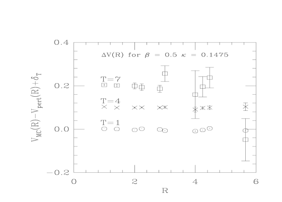
Figure 2: The difference between the measured and fitted effective potentials for $T=1$, $4$ and $7$, for $\beta=0.5$, $\lambda=0.01$ and $\kappa=0.1475$. The values for $T=4$ and $7$ have been displaced by $\delta_{T}=0.1$ and 0.2 vertically for better viewing.

As can be seen from Table 1 the results from normal and smeared loops agree within errors with the smeared loops giving somewhat smaller errors. The dependence on $\kappa$, i.e., the scalar fields, is rather weak with $g^{2}_{R}$ decreasing slightly as the scalars become lighter (as the Higgs transition is approached) as one would expect.

In Table 1 no $g^{2}_{R}$ is quoted for normal Wilson loops for $\beta=-0.5$. The reason is that several loops, including the plaquette, were negative there. In fact, exactly those of the small loops were negative, that would become positive under the transformation that makes the symmetry $\beta\to-\beta$ for the Wilson model, i.e., without the suppression of monopoles. Smearing got rid of this problem. However, the Wilson loops remained rather noisy compared to those obtained at positive gauge coupling and the approach to an asymptotic value of the effective potentials (13) was not monotonic. This fact points to a non–positive transfer matrix, as one might expect for the imaginary bare gauge coupling one has for negative $\beta$. A similar, non–monotonic behavior was observed in the Higgs phase, as will be discussed further below. We should add here, that contrary to all other cases, only time separations up to $T=4$ could be included in the fit for $g^{2}_{R}$. For larger $T$ we did not get a signal for the effective potential except for the smallest distances.

In the Higgs phase, the potential is a screened, or Yukawa potential. There we made fits to finite $T$ approximants of the lattice Yukawa potential

$$V^{\rm MC}_{T}(\vec{R})=g^{2}_{R}\cdot V^{\rm Yuk}_{T}(\vec{R})~{},$$ (17)

obtained from lowest order Wilson loops with the vector boson propagator in $R_{\xi}$ gauge with $\xi=1$ given by

$$G_{\mu\nu}(p)=\frac{\delta_{\mu\nu}}{4\sum_{\mu}\sin^{2}\frac{p_{\mu}}{2}+4\sinh^{2}\frac{\mu_{\gamma}}{2}},$$ (18)

with $\mu_{\gamma}$ the mass of the gauge boson. We used as a fitting parameter $m_{\gamma}=2\sinh\frac{\mu_{\gamma}}{2}$.

$\beta$	$\kappa$	$n_{smear}$	$g^{2}_{R}$	$m_{\gamma}$	$\chi^{2}$/ndf
0.5	0.1506	0	2.77(5)	0.92(4)	1.009
0.5	0.1506	0	3.00(3)	1.12(2)	1.309
0.5	0.1506	7	2.93(1)	1.06(1)	1.112
0.5	0.1506	7	2.88(2)	1.02(2)	2.231
0.5	0.1525	0	3.00(1)	1.71(1)	0.461
0.5	0.1525	0	2.96(3)	1.69(3)	0.605
0.5	0.1525	7	2.89(2)	1.63(2)	0.499
0.5	0.1525	7	2.78(4)	1.55(3)	1.159
0.5	0.1550	0	3.00(3)	2.17(2)	0.735
0.5	0.1550	7	2.94(1)	2.13(1)	0.888
0.5	0.1550	7	2.94(2)	2.12(2)	2.256
0.5	0.1575	0	2.85(2)	2.42(2)	0.679
0.5	0.1575	0	2.84(4)	2.40(3)	1.170
0.5	0.1575	7	2.85(1)	2.42(1)	0.705
0.5	0.1575	7	2.85(1)	2.41(1)	1.396
2.5	0.1350	7	0.447(1)	0.415(8)	1.313
2.5	0.1375	7	0.445(1)	0.550(3)	0.315
2.5	0.1375	7	0.445(1)	0.550(3)	0.839

Table 3: The fit parameters from fits to the finite $T$ approximants to the lattice Yukawa potential, obtained from lowest order Wilson loops with a massive gauge boson propagator, for $\lambda=0.01$. The first line for each data set is the fit with smallest $\chi^{2}$/ndf, and the second line comes from $T=7$, unless the fits are identical.

These fits, tabulated in Table 3 and 4, worked well for the $\lambda=0.01$, $\beta=0.5$ data where $m_{\gamma}$ is relatively large and a plateau is achieved quite soon, but they worked much better for the data at the larger $\beta$ value, $\beta=2.5$. A sample fit is shown in Figure 3. Notice the violations of rotational symmetry, especially at short distances, which are well followed by the lattice Yukawa potential. A fit to the continuum Yukawa potential $\frac{1}{R}{\rm e}^{-m_{\gamma}R}$ would not have worked. For data in the Coulomb phase, the Yukawa fits, correctly gave a vanishing photon mass, within error.

$\beta$	$\kappa$	$n_{smear}$	$g^{2}_{R}$	$m_{\gamma}$	$\chi^{2}$/ndf
0.5	0.2150	4	2.98( 7)	0.43(13)	0.823
0.5	0.2175	4	2.94( 6)	0.42(10)	0.048
0.5	0.2200	4	2.93( 2)	0.40( 3)	0.671
0.5	0.2225	7	2.93( 2)	0.44( 3)	0.321
0.5	0.2250	4	2.93( 1)	0.46( 2)	0.031
2.5	0.1825	7	0.449(1)	0.119( 8)	0.478
2.5	0.1850	7	0.448(1)	0.154(14)	0.031
2.5	0.1875	7	0.448(1)	0.179(16)	0.790

Table 4: The fit parameters from fits to the finite $T$ approximants to the lattice Yukawa potential, obtained from lowest order Wilson loops with a massive gauge boson propagator, for $\lambda=3.0$.

Figure 3: Monte Carlo potential from smeared Wilson loops and the fit to the effective potential extracted from lowest order perturbative Wilson loops with a massive propagator, for $\beta=2.5$, $\lambda=0.01$ and $\kappa=0.1375$.

It maybe worthwhile to note that the attempt to fit to the ‘naive’ lattice Yukawa potential, the $T\to\infty$ limit of $V^{\rm Yuk}_{T}(\vec{R})$,

$$V_{naive}(\vec{R})=V_{0}+g^{2}_{R}\frac{1}{L^{3}}\sum_{\vec{p}}\frac{1-\cos(\vec{p}\vec{R})}{4\sum_{1\leq k\leq 3}\sin^{2}\frac{p_{k}}{2}+m^{2}_{\gamma}}$$ (19)

was successful only for $\lambda=0.01$ and $\beta=0.5$. For $\beta=2.5$ and both values of $\lambda$, as well as for $\beta=0.5$ and $\lambda=3.0$ we could not obtain fits with a decent $\chi^{2}$ using eq. (19). This observation is in disagreement with some statements in the literature [8]. A possible explanation might be that smaller statistical errors in our case lead to a better discrimination between different fit formulae, thus excluding the ‘naive’ fits.

In the quasiclassical perturbative approach one expects

$$m^{2}_{\gamma}\simeq\frac{2\kappa}{\beta}\cdot\langle\phi^{\ast}\phi\rangle.$$ (20)

Perturbative arguments suggest that this equality should be valid in the weak coupling region when the dimensionless mass $~{}\mu_{\gamma}~{}$ is sufficiently small, i.e., $~{}m_{\gamma}\simeq\mu_{\gamma}$. It is interesting to note that this equality seems to hold even in the region where $~{}m_{\gamma}~{}$ is not very small. In Figure 4 we compare the values of $~{}m_{\gamma}~{}$ taken from Table 3 with that calculated via eq. (20) at $~{}\beta=0.5~{}$ and $~{}\lambda=0.01$. Qualitatively, the agreement is quite reasonable, indicating consistency of the quasiclassical estimation.

Figure 4: The parameter $m_{\gamma}$ in the Higgs phase. Diamonds correspond to $m_{\gamma}$ values taken from Table 3. The solid line corresponds to r.h.s. of eq. (20).

For $\beta=-0.5$ the potentials looked rather strange, with the point at $R=1$ being the highest. An example is shown in Figure 5. The potentials from smeared and normal Wilson loops, where available, agreed. As in the Coulomb phase, the potential approximants show a non–monotonic behavior with $T$, though a plateau is reached rather quickly. Even ignoring the $R=1$ point, no good fits could be obtained, and hence no conclusions drawn.

Figure 5: Monte Carlo potential from smeared Wilson loops for $\beta=-0.5$, $\lambda=0.01$ and $\kappa=0.1875$.

4.2 Screening Energy

The gauge invariant two–point function (11) can be interpreted as an external static charge propagating forward in (Euclidean) time. The presence of the external charge manifests itself as an energy increase $\mu$ of the lowest state of the system. The screening of an external source may be studied from the exponential fall–off of $G(T,R)$ for fixed $R$ and for $T$ large enough:

$$G(T,R)\sim f(R)\exp(-\mu T).$$ (21)

For smaller $T$ there are subleading exponentials to this. $\mu$ is the lowest energy in the fields that screen an external charge, and is therefore called the screening energy.

In a confining phase in the presence of matter fields or in the Higgs phase, the external charges are always completely screened and one therefore finds that

$$\mu=\frac{1}{2}V(\infty)$$ (22)

with $V(R)$ the static potential that can be extracted from Wilson loops. In the Coulomb phase the screening energy is the energy of a bound–state of a light charge, represented by the field $\phi^{*}$ in (11) and the static charge, corresponding to the straight time–like segment. With $m_{c}$ the mass of the light charged particle the screening energy is then

$$\mu=\frac{1}{2}V(\infty)+m_{c}-E_{b}$$ (23)

with $E_{b}$ the binding energy. One therefore expects $\mu>V(\infty)/2$ in the Coulomb phase.

$\beta,~{}\kappa\setminus\mu$	$R=1$	$R=2$	$R=3$	$R=4$	$\frac{1}{2}V(R=4)$
-0.5, 0.1850	0.1635(1)	0.1634(1)	0.1632(3)	0.1630(3)	0.1637(10)
-0.5, 0.1875	0.1325(1)	0.1327(1)	0.1330(2)	0.1329(2)	0.1322(5)
-0.5, 0.1900	0.1123(1)	0.1128(2)	0.1128(2)	0.1129(3)	0.1117(3)
0.5, 0.1450	1.25(16)	0.94(25)	1.37(32)	1.60(10)	0.34(1)
0.5, 0.1475	1.00(5)	0.76(7)	0.68(35)	0.57(49)	0.32(1)
0.5, 0.1500	0.63(5)	0.65(5)	0.59(10)	0.47(10)	0.33(1)
0.5, 0.1506	0.2437(5)	0.2442(6)	0.2447(8)	0.2412(10)	0.242(3)
0.5, 0.1525	0.1844(2)	0.1841(2)	0.1842(3)	0.1842(4)	0.183(1)
0.5, 0.1550	0.1484(1)	0.1486(1)	0.1487(2)	0.1485(3)	0.1487(6)
0.5, 0.1575	0.1264(1)	0.1265(1)	0.1264(1)	0.1263(1)	0.1267(3)

Table 5: Screening energy $\mu$ for $\lambda=0.01$ extracted from fits with unsmeared operators for different $R$ values and $\kappa$, generally with $T\geq 4$.

$\beta,~{}\kappa\setminus\mu$	$R=1$	$R=2$	$R=3$	$R=4$	$\frac{1}{2}V(R=4)$
-0.5, 0.1850	0.1635(1)	0.1637(1)	0.1637(1)	0.1637(1)	0.1634(2)
-0.5, 0.1875	0.1324(1)	0.1325(1)	0.1326(1)	0.1326(1)	0.1323(1)
-0.5, 0.1900	0.1124(1)	0.1124(1)	0.1122(1)	0.1124(1)	0.1123(1)
0.5, 0.1450	1.31(13)	0.73(12)	1.49(7)	1.37(7)	0.332(1)
0.5, 0.1475	1.05(6)	0.98(6)	1.00(9)	1.05(10)	0.332(2)
0.5, 0.1500	0.64(5)	0.65(5)	0.49(4)	0.64(7)	0.329(2)
0.5, 0.1506	0.2435(5)	0.2438(6)	0.2438(6)	0.2430(6)	0.2426(7)
0.5, 0.1525	0.1841(2)	0.1840(3)	0.1842(3)	0.1845(2)	0.1838(3)
0.5, 0.1550	0.1484(1)	0.1484(1)	0.1485(1)	0.1485(2)	0.1485(2)
0.5, 0.1575	0.1263(1)	0.1264(1)	0.1264(1)	0.1264(1)	0.1263(2)

Table 6: Screening energy $\mu$ for $\lambda=0.01$ extracted from fits with smeared operators for different $R$ values and $\kappa$, with $T\geq 4$.

The gauge–invariant two–point function $G(T,R)$ could be calculated quite accurately and showed in both the free charge phase and the Higgs phase the expected exponential falloff as a function of $T$, for $T$ large enough with $R$ fixed as in eq. (21). Figure 6 shows the behavior of the two–point function as a function of $T$ and different $R$ for $\kappa=0.1506$, $\beta=0.5$ and $\lambda=0.01$ near the phase transition. The screening energy, as extracted from different distances $R$, is tabulated in Tables 5 and 6 for unsmeared and smeared operators, respectively. The last column in both Tables is an estimation of the selfenergy of an isolated charge $E_{q}=\frac{1}{2}V(R=\infty)$ from the potential $V(R=4,T=5)$. The screening energy as defined by eq. (21) is supposed to be independent of the distance $R$ in the gauge invariant two–point function $G(T,R)$ [9]. Our results are in general agreement with this expectation. In the Coulomb phase, where $\mu$ is rather large and hence less well determined since $G(T,R)$ becomes noisier at larger $T$, there are some variations, but clearly no definite trend. We also note that both smeared and unsmeared operators work equally well leading to consistent values of $\mu$, except for the ‘problem points’ mentioned above. We therefore expect that with much better statistics $\mu$ would again turn out to be independent of $R$.

In Figure 7, we show the screening energy $\mu$ as a function of $\kappa$, extracted from fits to $\log(G(T,R))$. Also shown in the figure is $V(R=4)/2$, our approximation to $E_{q}=V(\infty)/2$, the selfenergy of an isolated external charge. In the Higgs phase, $V(R=4)/2$ is expected to be an excellent approximation to $V(\infty)/2$, and as expected $\mu$ and $V(\infty)/2$ agree very well, (22). In the Coulomb phase, $V(\infty)/2$ is slightly higher than $V(R=4)/2$ but, as expected, the screening energy $\mu$ is clearly much larger.

Figure 6: The logarithm of $G(T,R)$ plotted as a function of $T$ for various $R$ at $\kappa=0.1506$, $\beta=0.5$ and $\lambda=0.01$ .

Figure 7: The screening energy $\mu$ and the selfenergy of an isolated external charge, $E_{q}$, approximated by $V(R=4)/2$, as a function of $\kappa$ for $\beta=0.5$ and $\lambda=0.01$. $\mu$ is determined from the exponential decay of $G(T,R=1)$.

For $\lambda=3.0$ and all $\beta$–values, and for $\lambda=0.01$ at $\beta=2.5$, due to an oversight we only computed $G(R,T)$ used for the Fredenhagen–Marcu order parameter, but not $G(T,R)$. Therefore we have no data for the screening energy for those parameter values.

4.3 Fredenhagen–Marcu Order Parameter

Fredenhagen and Marcu found that a suitable criterion to study confinement in gauge theories with matter fields [21] can be formulated in terms of the ratio

$$\rho_{FM}(R,T)=\frac{G(R,T)}{W(R,2T)^{1/2}}.$$ (24)

This ratio has the asymptotic behavior

$$\rho_{FM}(R,T)\mathop{\longrightarrow}\limits_{\scriptscriptstyle R\to\infty,T=R/2}\left\{\begin{array}[]{ll}\rho_{FM}^{\infty}{}{}{}{}{}&\mbox{confined or Higgs phase}\\ 0&\mbox{Coulomb phase}\end{array}\right.~{}~{}~{}.$$ (25)

The physical interpretation is that one of two charges is removed as $R\to\infty$. If free charges can exist the overlap of the remaining one–charge state with the vacuum is zero and the ratio (24) vanishes. If the remaining charge is screened as in a confined or Higgs phase the ratio attains a finite, non–zero limit. In both cases the division by the Wilson loop ensures the cancellation of the perimeter law behavior in $G(R,T)$. The asymptotic value $\rho_{FM}^{\infty}$ is therefore called the vacuum overlap order parameter. The ratio between $T$ and $R$ is held fixed in the limiting process to ensure projection onto the state with lowest energy.

The Fredenhagen–Marcu parameter $\rho_{FM}(R,T)$ turns out to be a very good parameter signalling the Higgs phase transition [9]. As our lattices were restricted to $8^{3}\times 16$, we were able to calculate this only up to $\rho_{FM}(4,2)$. But as Figures 8 to 11 indicate, this quantity behaves like an order parameter.

Figure 8: The Fredenhagen–Marcu parameter $\rho_{FM}(R,T)$ as a function of $\kappa$ for $\beta=0.5$ and $\lambda=0.01$.

Figure 9: The Fredenhagen–Marcu parameter $\rho_{FM}(R,T)$ as a function of $\kappa$ for $\beta=2.5$ and $\lambda=0.01$.

Figure 10: The Fredenhagen–Marcu parameter $\rho_{FM}(R,T)$ as a function of $\kappa$ for $\beta=0.5$ and $\lambda=3.0$.

Figure 11: The Fredenhagen–Marcu parameter $\rho_{FM}(R,T)$ as a function of $\kappa$ for $\beta=2.5$ and $\lambda=3.0$.

Our data for $\lambda=0.01$ are tabulated in Table 7 from computations with normal and smeared space–like links and in Table 8 for $\lambda=3.0$ with smeared space–like links.

$\beta,~{}\kappa\setminus\rho_{FM}$	$R=2$,norm	$R=4$,norm	$R=2$,smear	$R=4$,smear
-0.5, 0.1850	0.278(2)	0.007(6)	0.0542(4)	0.0030(8)
-0.5, 0.1875	21.137(5)	13.886(5)	15.082(3)	13.015(3)
-0.5, 0.1900	19.12(4)	19.19(6)	17.308(3)	15.279(3)
0.5, 0.1450	0.0654(2)	0.0024(3)	0.0420(1)	0.0025(1)
0.5, 0.1475	0.0786(3)	0.0041(3)	0.0510(2)	0.0045(2)
0.5, 0.1500	0.091(4)	0.020(3)	0.102(5)	0.036(6)
0.5, 0.1506	1.89(2)	1.93(2)	1.88(2)	1.91(2)
0.5, 0.1525	4.47(1)	2.673(9)	4.148(9)	4.19(1)
0.5, 0.1550	5.556(5)	4.652(5)	6.217(5)	6.258(6)
0.5, 0.1575	6.636(2)	5.254(2)	7.923(3)	7.952(3)
2.5, 0.1275			0.0433(2)	0.0034(3)
2.5, 0.1300			0.0530(4)	0.0080(6)
2.5, 0.1325			0.36(1)	0.30(1)
2.5, 0.1350			1.536(4)	1.424(3)
2.5, 0.1375			2.654(2)	2.496(2)

Table 7: The Fredenhagen–Marcu parameter $\rho_{FM}(R,T)$ for $\lambda=0.01$ extracted from unsmeared (normal) and smeared operators for $R=2$ and $R=4$ with $T=R/2$.

$\beta,~{}\kappa\setminus\rho_{FM}$	$R=2$	$R=4$
-0.5, 0.3150	0.122(2)	0.057(7)
-0.5, 0.3175	0.135(4)	0.06(1)
-0.5, 0.3200	0.171(5)	0.116(8)
-0.5, 0.3225	0.235(5)	0.28(1)
-0.5, 0.3250	0.287(3)	0.311(7)
-0.5, 0.3275	0.335(3)	0.371(6)
0.5, 0.2100	0.0574(3)	0.0132(6)
0.5, 0.2125	0.0665(8)	0.021(1)
0.5, 0.2150	0.090(2)	0.049(2)
0.5, 0.2175	0.1465(8)	0.118(1)
0.5, 0.2200	0.1913(7)	0.171(1)
0.5, 0.2225	0.2266(5)	0.2126(8)
0.5, 0.2250	0.2610(4)	0.2504(5)
2.5, 0.1750	0.0463(5)	0.0090(9)
2.5, 0.1775	0.058(1)	0.020(2)
2.5, 0.1800	0.103(2)	0.071(2)
2.5, 0.1825	0.1465(7)	0.1186(9)
2.5, 0.1850	0.1823(4)	0.1574(5)
2.5, 0.1875	0.2149(3)	0.1921(3)

Table 8: The Fredenhagen–Marcu parameter $\rho_{FM}(R,T)$ for $\lambda=3.0$ extracted from smeared operators for $R=2$ and $R=4$ with $T=R/2$.

5 Spectrum Calculations

To probe the spectrum of the model, we constructed correlation functions of the following operators:

$${\cal O}_{S}({\bf x},t) = {\rm Re}\sum_{\mu}\phi_{x}^{*}U_{x,\mu}\phi_{x+\hat{\mu}}$$ (26)

$${\cal O}_{V}({\bf x},t) = {\rm Im}\sum_{\mu}\phi_{x}^{*}U_{x,\mu}\phi_{x+\hat{\mu}}$$ (27)

$${\cal O}_{P}({\bf x},t) = {\rm Im}\sum_{\Box}U_{\Box}$$ (28)

with the subscripts $S$, $V$, and $P$ corresponding to the scalar boson, the vector boson and the photon, and $\mu,\nu=1,2,3$. These states have $J^{PC}$ quantum numbers $0^{++}$, $1^{--}$ and $1^{+-}$ respectively. The operator ${\cal O}_{P}$ at momentum $p=0$ has the wrong parity for a photon state. However, at non–zero momenta, $p>0$, parity is no longer a good quantum number for extended objects like the plaquettes, $U_{\Box}$, and ${\cal O}_{P}$ will have non–zero overlap with photon states [22].

To study the spectrum of the model, we extract the connected correlations of a generic operator ${\cal O}$ with quantum numbers $J^{PC}$ and momentum $\vec{p}$:

$$C(\tau) = \langle{\cal O}(t+\tau;{\vec{p}}){\cal O}^{\dagger}(t;{\vec{p}})\rangle-\langle{\cal O}(t+\tau;{\vec{p}})\rangle\langle{\cal O}^{\dagger}(t;{\vec{p}})\rangle;$$

$${\cal O}(t;{\vec{p}}) = \sum_{{\vec{x}}}e^{i{\vec{x}}{\vec{p}}}\cdot{\cal O}(t;{\vec{x}}).$$

These correlations are a sum of exponentials exp$(-E_{i}\tau)$ with $E_{i}$ the energies of the different states with the given quantum number. We are interested in the state with the lowest energy, $E_{0}$, in each channel. This lowest energy can be approximated by the effective energy

$$E_{eff}=-\ln\frac{C(\tau)}{C(\tau-1)},$$ (30)

at large enough $\tau$ with $\tau\ll L_{t}/2$. In practice, the situation is more complicated as the signals for larger time–slices die away rapidly. The true energy $E$ could be quite different from the calculated energy $E_{eff}$ if there is a lot of contamination from the higher energy states. In order to maximize the overlap of the lowest lying state with our operator and obtain a better signal for the effective energies, we used the APE smearing technique and applied between five and ten smearing iterations. In our computations, we found that we were able to get reliable signals up to $\tau=2$. Once the energies $E$ have been determined, the masses of the corresponding particles may be calculated through the lattice dispersion relation:

$$\sinh^{2}\frac{aE}{2}=\sinh^{2}\frac{am}{2}+\sum_{i=1}^{3}\sin^{2}\frac{ap_{i}}{2}.$$ (31)

The momenta, here, are given by $p_{i}=2\pi k_{i}/(aL)$, with $k_{i}=-\frac{1}{2}L+1,\ldots,\frac{1}{2}L$. We shall refer to these momenta simply as “$p_{i}=k_{i}$” or as “$p=k$”, keeping in mind that the momenta are given in units of $2\pi/(aL)$.

5.1 Photon

The operator ${\cal O}_{P}$, which at non–zero momentum couples to the photon, was measured at several non–zero momenta. The results for the effective energy at different $\beta$ and $\lambda$ are tabulated in Tables 9 to 11. As an example, we show in Figure 12 the effective energies for 3 different momenta for $\lambda=0.01$ and $\beta=0.5$. The lines correspond to the effective energies that would be expected for a massless particle at these 3 momenta. As expected, the photon is massless at $\kappa$’s smaller than $\kappa_{c}$ (in the Coulomb phase) and acquires a mass at $\kappa>\kappa_{c}$ (in the Higgs phase). This mass, extracted from the energy with the dispersion relation (31), is given in the last three columns of Tables 9 to 11. We note that the masses extracted from the dispersion relation are in general agreement with, though somewhat smaller than, those from the Yukawa fits to the potential (see Tables 3 and 4), but they tend to have larger errors. The dependence of the photon mass on $\kappa$ above the phase transition (PT) is rather strong for small self–coupling, i.e., $\lambda=0.01$, and a discontinuity of the mass can not be excluded. On the contrary, for large self–coupling ($\lambda=3.0$) the photon mass grows very slowly above the PT, in agreement with a previous observation in [10].

The study of other order parameters in the previous sections convinced us that a massless state should exist also at negative $\beta$’s ($\beta>-0.7$). This is indeed the case. As an illustration we show in Figure 13 the effective energies for different momenta for $\lambda=3.0$ and $\beta=-0.5$.

Figure 12: Effective Energies of the $1^{+-}$ state at three different non–zero momenta as indicated for $\lambda=0.01$ and $\beta=0.5$. The lines correspond to the effective energies expected from a massless particle.

Figure 13: Effective Energies of the $1^{+-}$ state at three different momenta indicated for $\lambda=3.0$ and $\beta=-0.5$. The solid lines correspond to the effective energies expected from a massless particle.

$\beta,\kappa$	$E_{k=1}$	$E_{k=2}$	$E_{k=3}$	$m_{k=1}$	$m_{k=2}$	$m_{k=3}$
-0.5, 0.1850	0.74(2)	1.33(5)	1.78(8)
0.5, 0.1450	0.75(1)	1.29(4)	1.57(8)
0.5, 0.1475	0.75(1)	1.35(4)	1.72(7)
0.5, 0.1500	0.756(6)	1.30(5)	1.72(11)
0.5, 0.1506	1.15(3)	1.51(5)	2.00(13)	0.91(4)	0.84(11)	1.3(3)
0.5, 0.1525	1.64(11)	2.22(17)	2.75(49)	1.51(13)	1.97(22)	2.5(6)
0.5, 0.1550	2.01(13)	1.80(14)	1.80(20)	1.93(14)	1.38(22)	0.9(6)
0.5, 0.1575	2.14(14)	1.94(15)	3.09(97)	2.07(15)	1.59(22)	2.9(1.2)

Table 9: The effective energies and, in the Higgs phase, the extracted masses of the photon from unsmeared operators at time–slice 2 for $\lambda=0.01$ and for three different values of the momentum: $\vec{k}=(0,1,0)$, $\vec{k}=(0,2,0)$ and $\vec{k}=(0,3,0)$.

$\beta,\kappa$	$E_{k=1}$	$E_{k=2}$	$E_{k=3}$	$m_{k=1}$	$m_{k=2}$	$m_{k=3}$
-0.5, 0.1850	0.72(1)	1.32(9)
-0.5, 0.1875	0.68(11)	1.30(49)
0.5, 0.1450	0.749(8)	1.28(3)	1.66(6)
0.5, 0.1475	0.75(1)	1.34(3)	1.71(9)
0.5, 0.1500	0.754(7)	1.30(3)	1.66(8)
0.5, 0.1506	1.18(2)	1.55(4)	1.90(13)	0.95(3)	0.93(8)	1.1(3)
0.5, 0.1525	1.62(4)	1.95(9)	2.19(19)	1.49(5)	1.60(13)	1.7(3)
0.5, 0.1550	2.03(10)	1.82(9)	1.90(14)	1.95(11)	1.41(14)	1.1(3)
0.5, 0.1575	2.06(11)	1.95(10)	2.85(33)	1.98(12)	1.60(14)	2.6(4)
2.5, 0.1275	0.758(8)	1.33(4)	1.60(8)
2.5, 0.1300	0.75(1)	1.33(4)	1.44(5)
2.5, 0.1325	0.76(1)	1.39(4)	1.72(8)	0.14(6)	0.51(14)	0.6(4)
2.5, 0.1350	0.84(2)	1.30(4)	1.63(7)	0.40(5)
2.5, 0.1375	0.90(2)	1.40(5)	1.78(7)	0.52(4)	0.54(17)	0.8(2)

Table 10: The effective energies and, in the Higgs phase, the extracted masses of the photon from smeared operators at time–slice 2 for $\lambda=0.01$ and for three different values of the momentum: $\vec{k}=(0,1,0)$, $\vec{k}=(0,2,0)$ and $\vec{k}=(0,3,0)$.

$\beta,\kappa$	$E_{k=1}$	$E_{k=2}$	$E_{k=3}$	$m_{k=1}$	$m_{k=2}$	$m_{k=3}$
-0.5, 0.3150	0.72(4)	1.29(14)	1.04(1.96)
-0.5, 0.3175	0.74(4)	1.20(18)
-0.5, 0.3200	0.78(4)	1.16(11)	0.7(1.02)	0.23(15)
-0.5, 0.3225	0.78(5)	1.37(15)		0.23(18)	0.4(6)
-0.5, 0.3250	0.84(3)	1.40(18)	1.08(1.43)	0.40(7)	0.5(6)
-0.5, 0.3275	0.91(5)		1.72(29)	0.54(9)
0.5, 0.2100	0.740(9)	1.30(4)	1.51(12)
0.5, 0.2125	0.75(1)	1.25(5)	1.49(11)
0.5, 0.2150	0.76(1)	1.28(3)	1.71(7)	0.14(6)		0.5(3)
0.5, 0.2175	0.79(1)	1.32(4)	1.74(10)	0.27(3)		0.7(4)
0.5, 0.2200	0.82(1)	1.36(4)	1.79(14)	0.35(3)	0.39(18)	0.8(4)
0.5, 0.2225	0.85(1)	1.34(5)	1.62(12)	0.42(2)	0.3(3)
0.5, 0.2250	0.86(1)	1.41(5)	1.72(10)	0.44(2)	0.58(16)	0.6(4)
2.5, 0.1750	0.78(1)	1.39(4)	1.66(7)
2.5, 0.1775	0.74(1)	1.30(4)	1.66(6)
2.5, 0.1800	0.72(1)	1.36(3)	1.67(6)
2.5, 0.1825	0.75(1)	1.22(2)	1.85(8)	0.06(14)		1.0(2)
2.5, 0.1850	0.75(1)	1.27(4)	1.55(6)	0.06(14)
2.5, 0.1875	0.77(1)	1.43(5)	1.56(7)	0.19(4)	0.64(15)

Table 11: The effective energies and, in the Higgs phase, the extracted masses of the photon from smeared operators at time–slice 2 for $\lambda=3.0$ and for three different values of the momentum: $\vec{k}=(0,1,0)$, $\vec{k}=(0,2,0)$ and $\vec{k}=(0,3,0)$.

5.2 Scalar Boson

It is rather plausible that in the Coulomb phase the scalars $\phi$ interacting through the attractive Coulombic force and the $\phi^{4}$ coupling can form massive bound–states, bosonium, analogous to positronium in normal (fermionic) QED. One of the possible bound–states has the same quantum numbers, $0^{++}$, as the Higgs boson in the Higgs phase. The analogy with positronium makes it interesting to subject this state to a somewhat detailed study. Therefore, we attempted to check its lattice dispersion relation at different $\beta$ and $\lambda$, including the negative value $\beta=-0.5$.

We measured at two different momenta, $p=0$ and $p=1$. We were especially interested to see whether a two free particles dispersion (DR) relation was to be favored over a single–particle dispersion, indicating a bound–state, in the Coulomb phase. To investigate this, we calculated the mass of the two assumed free particles from the $p=0$ energy ($E^{p=0}=2m$) and used this mass to compute the energy $E_{two}^{p=1}$ of the combined two–particle $p=1$ state,

$$E_{two}^{p=1}=m+(2/a){\rm arsinh}\sqrt{\sinh^{2}\frac{am}{2}+\sin^{2}\frac{\pi}{L}}.$$ (32)

We then compared the measured energy $E_{m}^{p=1}$ with the calculated energy $E_{two}^{p=1}$ as well as with the calculated energy $E_{sing}^{p=1}$ based on the one–particle dispersion relation. The results are tabulated in Tables 12 to 14, and shown in Figures 14 to 19.

In the Higgs phase the two–particle dispersion relation definitely fails, while the single–particle dispersion relation is quite consistent for the two different momenta $p$ we have chosen. This is, of course, consistent with the notion that the Higgs boson, in our model, is an elementary particle.

However, in the Coulomb phase the situation is less clear. Neither the single nor the two–particle dispersion relations work satisfactorily in the case of the strong self–interaction ($\lambda=3.0$). As an example, we show in Figures 14 and 15 the measured and calculated energies with two–particle DR and one–particle DR, respectively. The failure of the one–particle DR becomes even more pronounced for negative $\beta$’s (see Figures 16 and 17 ). A possible explanation could be that, in the Coulomb phase, our energy measurements are more contaminated by higher excitations. Unfortunately our signal does not allow us to go to larger $\tau$ to settle this issue.

Figure 14: Measured and calculated Energies of the $0^{++}$ state at $p=1$ assuming a two–particle dispersion relation for $\lambda=3.0$ and $\beta=2.5$.

Figure 15: Measured and calculated Energies of the $0^{++}$ state at $p=1$ assuming a single–particle dispersion relation for $\lambda=3.0$ and $\beta=2.5$.

Figure 16: Measured and calculated Energies of the $0^{++}$ state at $p=1$ assuming a two–particle dispersion relation for $\lambda=3.0$ and $\beta=-0.5$.

Figure 17: Measured and calculated Energies of the $0^{++}$ state at $p=1$ assuming a single–particle dispersion relation for $\lambda=3.0$ and $\beta=-0.5$.

In the case of weak self–interaction the one–particle DR looks somewhat preferable, as compared to the two–particle DR. In Figures 18 and 19 we show the measured and calculated energies with two–particle DR and one–particle DR, respectively, for $\beta=0.5$ and $\lambda=0.01$. A qualitatively similar picture was observed for other $\beta$–values for the same $\lambda$.

Figure 18: Measured and calculated Energies of the $0^{++}$ state at $p=1$ assuming a two–particle dispersion relation for $\lambda=0.01$ and $\beta=0.5$.

Figure 19: Measured and calculated Energies of the $0^{++}$ state at $p=1$ assuming a single–particle dispersion relation for $\lambda=0.01$ and $\beta=0.5$.

$\beta,\kappa\setminus E_{eff}$	$E_{meas}^{p=0}$	$E_{meas}^{p=1}$	$E_{two}^{p=1}$	$E_{sing}^{p=1}$
-0.5, 0.1850	1.65(11)	1.87(14)	1.91(9)	1.76(10)
-0.5, 0.1850(*)	0.93(3)	1.23(3)	1.33(2)	1.16(2)
-0.5, 0.1875	1.06(4)	1.35(4)	1.43(3)	1.26(3)
-0.5, 0.1900	1.17(12)	1.48(43)	1.52(10)	1.35(10)
0.5, 0.1450	1.84(17)	2.01(16)	2.07(15)	1.93(15)
0.5, 0.1475	1.64(10)	1.67(7)	1.90(9)	1.75(9)
0.5, 0.1500	0.42(9)	1.17(5)	0.99(6)	0.85(4)
0.5, 0.1506	0.33(2)	0.81(2)	0.93(1)	0.813(7)
0.5, 0.1525	0.66(3)	0.97(2)	1.14(2)	0.98(2)
0.5, 0.1550	0.91(3)	1.15(3)	1.32(2)	1.15(2)
0.5, 0.1575	1.07(5)	1.25(4)	1.44(4)	1.27(4)

Table 12: The effective energies of the $0^{++}$ scalar boson at momentum $p=0$ and $p=1$ from unsmeared operators at time–slice 2 for $\lambda=0.01$. Tabulated are the effective energies which were actually measured and for $p=1$ also those computed from a two–particle and from a single–particle dispersion relation for the given $E^{p=0}$. The (*) data corresponds to a run from a new start, starting from $\kappa=0.1875$.

$\beta,\kappa\setminus E_{eff}$	$E_{meas}^{p=0}$	$E_{meas}^{p=1}$	$E_{two}^{p=1}$	$E_{sing}^{p=1}$
-0.5, 0.1850	1.59(9)	1.91(15)	1.86(7)	1.71(8)
-0.5, 0.1850(*)	0.93(3)	1.24(3)	1.33(2)	1.16(2)
-0.5, 0.1875	1.07(4)	1.34(4)	1.44(3)	1.27(3)
-0.5, 0.1900	1.21(5)	1.47(4)	1.55(4)	1.38(4)
0.5, 0.1450	1.65(15)	1.99(13)	1.92(12)	1.76(13)
0.5, 0.1475	1.56(7)	1.60(6)	1.84(6)	1.68(6)
0.5, 0.1500	0.44(11)	1.16(6)	1.00(7)	0.86(5)
0.5, 0.1506	0.33(2)	0.81(2)	0.93(1)	0.813(7)
0.5, 0.1525	0.66(2)	0.98(1)	1.15(1)	0.98(1)
0.5, 0.1550	0.91(1)	1.17(2)	1.32(1)	1.15(1)
0.5, 0.1575	1.02(3)	1.27(3)	1.40(2)	1.23(2)
2.5, 0.1275	1.60(12)	1.82(17)	1.87(10)	1.72(11)
2.5, 0.1300	1.30(10)	1.56(11)	1.63(8)	1.46(8)
2.5, 0.1325	0.23(2)	0.84(2)	0.87(1)	0.780(7)
2.5, 0.1350	0.63(2)	0.96(2)	1.12(1)	0.96(1)
2.5, 0.1375	0.81(1)	1.10(2)	1.25(1)	1.08(1)

Table 13: The effective energies of the $0^{++}$ scalar boson at momentum $p=0$ and $p=1$ from smeared operators at time–slice 2 for $\lambda=0.01$. Tabulated are the effective energies which were actually measured and for $p=1$ also those computed from a two–particle and from a single–particle dispersion relation for the given $E^{p=0}$. The (*) data corresponds to a run from a new start, starting from $\kappa=0.1875$.

$\beta,\kappa\setminus E_{eff}$	$E_{meas}^{p=0}$	$E_{meas}^{p=1}$	$E_{two}^{p=1}$	$E_{sing}^{p=1}$
-0.5, 0.3150	0.80(12)	1.83(17)	1.24(9)	1.07(8)
-0.5, 0.3175	0.60(8)	1.43(12)	1.10(5)	0.94(5)
-0.5, 0.3200	0.52(4)	1.23(9)	1.05(3)	0.90(2)
-0.5, 0.3225	0.61(5)	1.05(7)	1.11(3)	0.95(3)
-0.5, 0.3250	0.76(5)	1.14(5)	1.21(3)	1.04(3)
-0.5, 0.3275	0.74(5)	1.04(4)	1.19(3)	1.03(3)
0.5, 0.2100	1.24(11)	1.43(9)	1.58(9)	1.41(9)
0.5, 0.2125	0.71(4)	1.30(8)	1.18(3)	1.01(2)
0.5, 0.2150	0.47(2)	1.16(4)	1.02(1)	0.87(1)
0.5, 0.2175	0.58(2)	1.15(5)	1.08(1)	0.93(1)
0.5, 0.2200	0.74(3)	1.14(3)	1.20(2)	1.03(2)
0.5, 0.2225	0.81(3)	1.17(4)	1.25(2)	1.08(2)
0.5, 0.2250	0.94(3)	1.20(4)	1.34(2)	1.17(2)
2.5, 0.1750	1.07(6)	1.54(8)	1.44(5)	1.27(5)
2.5, 0.1775	0.58(5)	1.32(10)	1.08(3)	0.93(3)
2.5, 0.1800	0.49(4)	1.07(4)	1.03(2)	0.88(2)
2.5, 0.1825	0.69(3)	1.10(3)	1.17(2)	1.00(2)
2.5, 0.1850	0.81(3)	1.15(5)	1.25(2)	1.08(2)
2.5, 0.1875	0.94(4)	1.20(5)	1.35(3)	1.17(3)

Table 14: The effective energies of the $0^{++}$ scalar boson at momentum $p=0$ and $p=1$ from smeared operators at time–slice 2 for $\lambda=3.0$. Tabulated are the effective energies which were actually measured and for $p=1$ also those computed from a two–particle and from a single–particle dispersion relation for the given $E^{p=0}$.

5.3 Vector Boson

Figure 20: Effective Energies of the $1^{--}$ vector boson at $p=1$ and $p=0$ for $\lambda=0.01$ and $\beta=0.5$.

Correlations of the operator ${\cal O}_{V}$ allow, in principle, the measurement of the $1^{--}$ vector boson mass. This works reasonably well in the Higgs phase. As an example, we show in Figure 20 the effective energies at $p=1$ and $p=0$ for $\beta=0.5$ and $\lambda=0.01$. All results are tabulated in Tables 15 and 16. There is a general tendency for the vector boson mass to decrease, as the Higgs transition is approached, just as is observed for the scalar boson. The signal–to–noise ratio is too big to disentangle the dispersion relations in a way we did for the scalar $~{}0^{++}~{}$ boson. Both one–particle dispersion relation and two–particle dispersion relation give consistent results within their error bars. Comparing with the masses extracted from the ‘photon’ operator ${\cal O}_{P}$ at non–zero momenta (Tables 9 to 11) we find rough agreement. Therefore, the two operators – ${\cal O}_{V}$ and ${\cal O}_{P}$ – seem to couple to the same state in the Higgs phase, the massive vector boson. This observation is in accordance with the perturbative analysis of the spectrum in the Higgs region, and confirms the early nonperturbative result [10] obtained in the case of strong self–coupling ($\lambda=3.0$).

In the Coulomb phase the situation is quite different from that in the Higgs phase. The correlators are very noisy and we do not have sufficient control of our signals to make, for example, an investigation of the existence of a bound–state like we attempted for the scalar boson. At non–zero momentum (there is no massless photon at zero momentum) the operator ${\cal O}_{V}$ should couple also to the photon. However, with rather large errors the effective energies for both $p=0$ and $p=1$ are both quite large, $\sim 2/a$, and comparable. The effective energy for $p=1$, in particular, is much larger than that of the photon, obtained from the correlations of ${\cal O}_{P}$. Evidently, the overlap with a photon state is very small. But due to the large errors on the effective energy, we can not make convincing arguments in favor of the existence of a vector bosonium in the Coulomb phase either. To settle the question of the excitation spectrum in the vector channel in the Coulomb phase would require much better statistics, or much better operators.

$\beta,\kappa$	$E^{norm}_{eff}(p=0)$	$E^{norm}_{eff}(p=1)$	$E^{smear}_{eff}(p=0)$	$E^{smear}_{eff}(p=1)$
0.5, 0.1450			1.85(35)	1.42(22)
0.5, 0.1475	1.48(36)		1.68(37)	2.16(38)
0.5, 0.1500	1.79(31)	1.34(15)	1.83(28)	1.37(13)
0.5, 0.1506	1.13(3)	1.28(36)	1.06(2)	1.41(6)
0.5, 0.1525	1.44(11)	1.75(11)	1.49(7)	1.79(11)
0.5, 0.1550	1.77(10)	1.90(12)	1.71(10)	2.03(13)
0.5, 0.1575	2.10(11)	2.25(31)	2.08(11)	2.30(27)
2.5, 0.1275			2.22(87)	2.6(1.6)
2.5, 0.1300			1.45(21)	2.6(1.0)
2.5, 0.1325			0.47(4)
2.5, 0.1350			0.42(1)	1.13(12)
2.5, 0.1375			0.56(1)	0.90(6)

Table 15: The effective energies for the $1^{--}$ vector boson from unsmeared (normal) and smeared operators at time–slice 2 for $\lambda=0.01$. There was no signal for entries left blank, and none at all for $\beta=-0.5$.

$\beta,\kappa$	$E_{eff}(p=0)$	$E_{eff}(p=1)$
-0.5, 0.3150	2.29(90)	1.18(23)
-0.5, 0.3175	1.69(55)	1.46(45)
-0.5, 0.3200	1.09(26)	1.31(41)
-0.5, 0.3225	1.11(26)	1.36(37)
-0.5, 0.3250	1.14(16)
-0.5, 0.3275	0.83(17)	2.0(1.5)
0.5, 0.2100
0.5, 0.2125	1.48(21)	1.49(23)
0.5, 0.2150	0.91(18)	1.65(39)
0.5, 0.2175	0.86(8)
0.5, 0.2200	0.68(5)	1.52(43)
0.5, 0.2225	0.68(5)	1.77(52)
0.5, 0.2250	0.66(3)	1.84(37)
2.5, 0.1750	1.89(44)	2.8(1.6)
2.5, 0.1775	1.49(26)	2.25(62)
2.5, 0.1800	0.90(19)
2.5, 0.1825	0.51(5)	2.7(1.2)
2.5, 0.1850	0.52(7)	2.3(1.3)
2.5, 0.1875	0.36(4)	2.4(1.2)

Table 16: The effective energies for the $1^{--}$ vector boson from smeared operators at time–slice 2 for $\lambda=3.0$. There was no signal for entries left blank.

6 Conclusions

We have made a thorough study of the compact $U(1)$ lattice gauge–Higgs model with completely suppressed monopoles. We studied it both for comparatively small self–coupling ($\lambda=0.01$), as well as in the strong self–coupling limit ($\lambda=\infty$ and $\lambda=3.0$). For strong self–coupling most computations were performed with $\lambda=3.0$, permitting us to compare our results with those of a previous study [9, 10] for the standard action. The computations were performed for three different values of the gauge coupling $\beta$: one at relatively weak gauge coupling, $\beta=2.5$, one at stronger coupling, $\beta=0.5$, and one at negative $\beta$, corresponding to imaginary bare gauge coupling.

We first mapped out the phase diagram of our model with monopoles suppressed. Contrary to the model with monopoles, it does not exhibit a confinement phase for strong gauge coupling. Nothing special seems to happen at $\beta=0$, and both Higgs and Coulomb phases continue to negative $\beta$ until about $\beta=-0.7$, where a first order transition into a frustrated phase seems to occur. The Higgs transition separating Coulomb and Higgs phase at positive $\beta$ is clearly of first order for $\lambda=0.01$, similar to what happens in the model with the standard action [7]. Following Coleman and Weinberg [23], it could be interpreted as a radiatively induced spontaneous symmetry breaking. At strong self–coupling the Higgs transition becomes weaker and its order harder to determine. From our data we can not exclude that the transition becomes second order for sufficiently large $\lambda$’s, similar to the non–compact case [12].

We measured $T$–dependent potentials from Wilson loops. In the Coulomb phase they could be well fit with a $T$–dependent Coulomb potential (extracted from perturbative Wilson loops), even at the negative $\beta$ probed, at least when the potential was extracted from smeared Wilson loops. The renormalized gauge coupling $g_{R}^{2}$ grows with decreasing $\beta$, and continues to rise rapidly at negative $\beta$. The suppression of monopoles therefore does not seem to exclude a strong–coupling QED, but shifts it to the (unphysical) region $g^{2}_{bare}<0$. Since there the bare coupling is imaginary the transfer matrix is no longer positive and it is thus not clear whether the model makes sense physically. However, we would like to stress again that we detected no indication of a phase transition between the positive and negative $\beta$ regions.

In the Higgs phase we fitted the $T$–dependent potentials to $T$–dependent Yukawa potentials. This worked well for positive $\beta$, and the extracted vector boson masses agreed reasonably with those obtained from conventional correlation functions. At negative $\beta$ the potential looked rather strange, and no good fits could be obtained.

To study the spectrum of the model we calculated the correlation functions corresponding to the photon (at non–zero momentum), the scalar boson with quantum numbers $0^{++}$ and the vector boson with $1^{--}$.

Our results conformed to our expectations, in particular for the photon. In the Coulomb phase it was found to be massless (even at negative $\beta$), and its energy fitted well the lattice dispersion relation. At $\kappa>\kappa_{c}$ (in the Higgs phase) the photon acquired a mass. The estimation of $\kappa_{c}$ from the behavior of the photon is in a good agreement with that obtained from the Fredenhagen–Marcu order parameter.

The measurements were more difficult for the $0^{++}$ and $1^{--}$ bosons, especially in the Coulomb phase. Both are reasonably well defined in the Higgs phase, as one would expect. Determination of the dispersion relation gave reasonably good evidence that the $0^{++}$ boson, the Higgs boson, is an elementary particle in the Higgs phase. In the Coulomb phase, however, the one–particle dispersion relation does not look very convincing, just like in the model with the standard action [9, 10]. Within our large errors a two–particle dispersion relation, appropriate for a weakly bound state, did not work much better. Therefore, we do not think that the problem of the existence of bosonium, a bound–state between two scalar particles, in the Coulomb phase is settled. Much better statistics and/or better operators are needed to settle this question.

References

- [1] K. Wilson, Phys. Rev. D10 (1974) 2445.
- [2] A. M. Polyakov, Nucl. Phys. B120 (1977) 429.
- [3] A. M. Polyakov, Gauge Fields and Strings, Harwood Academic Publishers (1987).
- [4] T. Banks and E. Rabinovici, Nucl. Phys. B160 (1979) 349.
- [5] E. Fradkin and S. Shenker, Phys. Rev. D19 (1979) 3682.
- [6] G. Koutsoumbas, Phys. Lett. B140 (1984) 379.
- [7] V.P. Gerdt, A.S. Ilchev and V.K. Mitrjushkin, Sov. J. Nucl. Phys. 43 (1986) 468.
- [8] K. Jansen, J. Jersák, C.B. Lang, T. Neuhaus and G. Vones, Phys. Lett. B155 (1985) 268; Nucl. Phys. B265 (1986) 129.
- [9] H.G. Evertz, V. Grösch, K. Jansen, J. Jersák, H.A. Kastrup and T. Neuhaus, Nucl. Phys. B285 (1987) 559.
- [10] H.G. Evertz, K. Jansen, J. Jersák, C.B. Lang and T. Neuhaus, Nucl. Phys. B285 (1987) 590.
- [11] P.H. Damgaard and U.M. Heller, Phys. Rev. Lett. 60 (1988) 1246.
- [12] M. Baig, H. Fort, J. B. Kogut and S. Kim, Phys. Rev. D51 (1995) 5216.
- [13] S. Dimopoulos, S. Raby and L. Susskind, Nucl. Phys. B173 (1980) 208.
- [14] E. Fahri and L. Susskind, Phys. Rep. 74 (1981) 277.
- [15] T. A. DeGrand and D. Toussaint, Phys. Rev. D22 (1980) 2478.
- [16] J. S. Barber, R. E. Schrock and R. Schrader, Phys. Lett. B152 (1985) 221.
- [17] V.G. Bornyakov, V.K. Mitrjushkin and M. Müller-Preussker, Nucl. Phys. B (Proc. Suppl.) 30 (1993) 587.
- [18] A. Hoferichter, V. K. Mitrjushkin and M. Müller-Preussker, Phys. Lett. B338 (1994) 325.
- [19] J. B. Kogut and L. Susskind, Phys. Rev. D9 (1974) 3501.
- [20] M. Albanese et al. (APE Collaboration), Phys. Lett. B192 (1987) 163.
- [21] K. Fredenhagen and M. Marcu, Commun. Math. Phys. 92 (1983) 81; Phys. Rev. Lett. 56 (1986) 223.
- [22] B. Berg and C. Panagiotakopoulos, Phys. Rev. Lett. 52 (1984) 94.
- [23] S. Coleman and E. Weinberg, Phys. Rev. D7 (1973) 1888.