Critical properties of the Antiferromagnetic
$\mathbf{R}\mathrm{P}^{2}$ model in three dimensions

Abstract

We study the behavior of the antiferromagnetic $\mathbf{R}\mathrm{P}^{2}$ model in $d=3$. The vacuum structure is analyzed in the critical and low temperature regions, paying special attention to the spontaneous symmetry breaking pattern. Near the critical point we observe a full breakdown of the $\mathrm{O}(3)$ symmetry of the action. Several methods for computing critical exponents are compared. We conclude that the most solid determination is obtained using a measure of the correlation length. Corrections-to-scaling are parameterized, yielding a very accurate determination of the critical coupling and a 5% error measure of the related exponent. This is used to estimate the systematic errors due to finite-size effects.

Keywords: Monte Carlo. $\mathbf{R}\mathrm{P}^{2}$. Nonlinear sigma model. Antiferromagnetism. Critical exponents. Finite size scaling.

PACS: 11.10.Kk;75.10.Hk;75.40.Mg.

1 Introduction.

Antiferromagnetic, (AF) interactions give rise to very interesting properties in statistical systems. Specifically, the symmetries of the broken AF phase can be very different from their ferromagnetic counterparts. Ground states with frustration or disorder are common in these systems.

oThe interest of AF models extends from the study of some physical problems where the antiferromagnetism appears naturally to the more theoretical aspects of new Spontaneous Symmetry Breaking (SSB) patterns, or Universality Classes. Moreover, attention has been recently paid to AF models in four dimensions [1, 2]. There, one could even hope to gain some insight on the puzzling problem of the non perturbative formulation of interacting field theories.

In this paper we will be concerned with the $\mathbf{R}\mathrm{P}^{2}$ model in three dimensions. Its ferromagnetic sector has been extensively used to study liquid crystals [3]. The AF one has been also studied [4, 5, 6] as it presents an unfrustrated ground state with nonzero disorder. It seems to belong to a class of models with a SSB pattern of type $\mathrm{SO}(3)\times\mathrm{SO}(2)/\mathrm{SO}(2)$ [6]. In condensed matter physics it is not rare to find systems with an equivalent SSB pattern, like super-fluid ³He [7], helical [8] and canted [9] spin systems and some frustrated quantum AF Heisenberg models [10], the latter being specially interesting because of their possible relation with High Temperature Superconductivity [11].

A radical reading of the Universality Hypothesis, suggests that the critical properties of a model are completely fixed by the space dimension and by its low and high temperature phase symmetry groups, $H$ and $G$ respectively. Even more, it is also generally assumed that models with locally isomorphic manifolds $G/H$ have identical critical behaviors, regardless of the global properties. This scenario has been theoretically challenged in ref. [12], where it has been suggested that the massive modes, not fixed by the local properties of $G/H$, could change the numerical values of the critical exponents.

The above SSB pattern has been studied in perturbation theory [13], where the main conclusions reached are that the only possible critical points in three dimensions are second-order, either with the Mean-Field (MF) exponents or with those of the $\mathrm{O}(4)$ sigma model, or first-order.

AF interactions frequently produce first-order transitions [14, 2], although with a large correlation length (weak-first-order transitions) that are characterized by the (apparent) critical exponents: $\nu=0.5$, $\gamma/\nu=2$, $\alpha/\nu=1$ [15]. These exponents are found in ref. [16] for the Stiefel manifold $V_{3,2}$. However, other Monte Carlo (MC) simulations for helical and canted spin models [8, 9, 17], have yielded exponents not far but incompatible with those of a weak-first-order transition.

On the other hand, the $\mathbf{R}\mathrm{P}^{2}$ antiferromagnetic model has a critical point with clearly different from weak-first-order exponents ($\nu\approx 0.78$, $\alpha/\nu\approx-0.44$) [6] and very close to those reported for $\mathrm{O}(4)$ [18], although hardly compatible with them.

The actual relevance of the model in experimental situations is difficult to know. It is an uneasy task to compare the critical exponents of this model with experimental data. In fact, the results for spin systems are not very clear, even regarding the order of the phase transitions encountered (see ref. [8] for a review). For the super-fluid ³He, the possibility of facing our critical exponents with experimental measures is remote, the critical region being so small that it seems experimentally inaccessible [19].

In this paper we present a more detailed exposition of the studies of ref. [6], completed with new analysis of the MC data. Our statistics have also increased by an amount of about a 50%. The high statistics has allowed a thorough study of the autocorrelation times, both exponential and integrated, for several observables. We are able to parameterize the corrections-to-scaling. As a consequence, we get a high precision determination of the critical point, and we measure the first correction-to-scaling exponent with an error of 5%. We use this exponent to extrapolate the critical exponents to their infinite-volume values, and get an estimation of the systematic errors. In addition, we carry out a study of the ordered phase both numerically and analytically. We find a low temperature phase with a global $\mathrm{O}(2)$ symmetry and, from finite-size scaling analysis, evidence of a breaking of this symmetry close to the transition. The MF approximation is considered at the critical point which already shows the extreme complexity of the symmetry-breaking pattern in that region. We also analyze the continuum limit of the model obtaining the $\mathrm{SO}(3)\times\mathrm{SO}(2)/\mathrm{SO}(2)$ non linear sigma model.

We start in section 2 by defining the model and the observables, and discuss some theoretical aspects and approximations. The MC algorithms used and the dynamics of the simulation are described in section 3. In section 4 we present a determination of the critical exponents using finite-size scaling techniques. The reliability of a parameterization of the corrections-to-scaling is considered in section 5. Finally sections 6 and 7 are devoted to discuss the vacuum structure of the broken phase. The conclusions are in section 8.

2 The Model.

We will consider a system of spins $\{\mbox{\boldmath$v$}_{i}\}$ taking values in the sphere $\mathrm{S}^{2}\subset\mathbf{R}^{3}$ and placed in the nodes of a cubic lattice. The interaction is defined by the action

$${\mathcal{S}}=-\beta\sum_{<i,j>}(\mbox{\boldmath$v$}_{i}\cdot\mbox{\boldmath$v$}_{j})^{2},$$ (1)

where the sum is extended over all pairs of nearest neighbor sites. The partition function is constructed as

$${\mathcal{Z}}=\int\left(\prod_{i}\mathrm{d}\mbox{\boldmath$v$}_{i}\right)\mathrm{e}^{-\mathcal{S}},$$ (2)

where the usual $\mathrm{O}(3)$-invariant measure is used.

The action and the measure are invariant under a local $\mathbf{Z}_{2}$ transformation ($\mbox{\boldmath$v$}_{i}\to-\mbox{\boldmath$v$}_{i}$). As this is a local symmetry, Elitzur’s Theorem guarantees its preservation even after a SSB. This means that the natural variable for the model is in an equivalent class of the quotient group $\mathbf{R}\mathrm{P}^{2}=\mathrm{S}^{2}/\mathbf{Z}_{2}$, the two-dimensional real projective space. The action (1) can be rewritten in terms of the $\mathbf{R}\mathrm{P}^{2}$ variables, which in turn can be expressed as the tensorial product of the original spins $\mbox{\boldmath$\tau$}_{i}=\mbox{\boldmath$v$}_{i}\otimes\mbox{\boldmath$v$}_{i}$,

$${\mathcal{S}}=-\beta\sum_{<i,j>}\mathop{\mathrm{tr}}\mbox{\boldmath$\tau$}_{i}\mbox{\boldmath$\tau$}_{j}.$$ (3)

As the measure for the $\tau$ is much more complex than for the vectors, it is generally more convenient to work directly with the latter.

2.1 Observables and measures.

The observables to be measure in a Monte Carlo simulation on a finite lattice must be scalars under the $\mathrm{O}(3)$ global symmetry group and obviously also under the local $\mathbf{Z}_{2}$ group. Let us construct the traceless tensorial field $\mathbf{T}_{i}$, whose components are

$$\mathrm{T}_{i}^{\alpha\beta}=v_{i}^{\alpha}v_{i}^{\beta}-\frac{1}{3}\delta^{\alpha\beta}.$$ (4)

The Fourier transform in a $L\times L\times L$ lattice can be defined as follows:

$$\widehat{\mathbf{T}}_{\mbox{\scriptsize\boldmath$p$}}=\sum_{\mbox{\scriptsize\boldmath$r$}\in L^{3}}\mathrm{e}^{-i\mbox{\scriptsize\boldmath$p$}\cdot\mbox{\scriptsize\boldmath$r$}}\ {\mathbf{T}}_{\mbox{\scriptsize\boldmath$r$}},$$ (5)

where we denote by $r$ the position vector of the site, and by $p$ the momentum ($\mbox{\boldmath$p$}=(2\pi n_{x}/L,2\pi n_{y}/L,2\pi n_{z}/L)$, with $n_{i}=0,\ldots,L-1$).

In principle, we are only interested in the magnetizations associated with a fixed momentum. In addition to the (normalized) zero momentum magnetization

$${\mathbf{M}}=\frac{1}{V}\sum_{x,y,z}{\mathbf{T}}_{(x,y,z)}=\frac{1}{V}\widehat{\bf T}_{(0,0,0)},$$ (6)

it is interesting to study the staggered magnetization related with states of period 2 under translations,

$${\bf M}_{\mathrm{s}}=\frac{1}{V}\sum_{x,y,z}(-1)^{x+y+z}{\mathbf{T}}_{(x,y,z)}=\frac{1}{V}\widehat{\mathbf{T}}_{(\pi,\pi,\pi)},$$ (7)

that is the (normalized) difference between the magnetization of the even sites, defined as those where $x+y+z$ is even, minus that of the odd ones, defined analogously.

Other finite momenta (nonzero in the $L\to\infty$ limit) could be necessary if the vacuum would present higher period symmetries. However we have not found any reason, neither analytical nor numerical, to expect this.

We compute the magnetization and the susceptibility respectively as

$$M=\left\langle\sqrt{\mathop{\mathrm{tr}}{\mathbf{M}}^{2}}\right\rangle,$$ (8)

$$\chi=V\left\langle\mathop{\mathrm{tr}}{\mathbf{M}}^{2}\right\rangle.$$ (9)

It is also useful to consider the quantity

$$\kappa=\frac{\langle\left(\mathop{\mathrm{tr}}\mathbf{M}^{2}\right)^{2}\rangle}{\langle\mathop{\mathrm{tr}}\mathbf{M}^{2}\rangle^{2}},$$ (10)

which is directly related with the Binder parameter [20].

We use the second momentum correlation length because it is easier to measure than the exponential (physical) one, but it is expected to have the same scaling behavior at the critical point [21, 22],

$$\xi=\left(\frac{\chi/F-1}{4\sin^{2}(\pi/L)}\right)^{1/2},$$ (11)

where $F$ is defined, using the shorthand notation $|\widehat{\mathbf{T}}|^{2}=\widehat{\mathbf{T}}\widehat{\mathbf{T}}^{\dagger}$, as

$$F=\frac{1}{3V}\left\langle\mathop{\mathrm{tr}}\left(\left|\widehat{\mathbf{T}}_{(\frac{2\pi}{L},0,0)}\right|^{2}+\left|\widehat{\mathbf{T}}_{(0,\frac{2\pi}{L},0)}\right|^{2}+\left|\widehat{\mathbf{T}}_{(0,0,\frac{2\pi}{L})}\right|^{2}\right)\right\rangle.$$ (12)

Analogously we define the associated quantities for the staggered observables.

We also measure the nearest neighbor energy

$$E_{1}=\frac{1}{3V}\sum_{<i,j>}(\mbox{\boldmath$v$}_{i}\cdot\mbox{\boldmath$v$}_{j})^{2},$$ (13)

and the next-to-nearest neighbor energy

$$E_{2}=\frac{1}{6V}\sum_{\ll i,j\gg}(\mbox{\boldmath$v$}_{i}\cdot\mbox{\boldmath$v$}_{j})^{2},$$ (14)

which is useful to study the $\mathrm{O}(3)$ broken phase.

The measures of $E_{1}$ have been also used to calculate the $\beta$ derivatives through its connected correlation with every observable.

2.2 The ground state.

When $\beta\gg 0$ the ground state corresponds to a configuration in which all the spins are aligned in a given direction. This state is thus $\mathrm{O}(2)$ invariant. The thermal fluctuations do not destroy this ordering until $\beta\sim 1.3$, where a first-order phase transition occurs. This system has been used for modeling liquid crystals [3].

For negative $\beta$, the ground state corresponds to a highly degenerated non-frustrated state where all spins are orthogonal to their neighbors.

The zero energy configurations that dominate the measure are those in which the even (odd) sublattice is aligned, and the spins in the odd (even) one lie randomly in the orthogonal plane. It is easy to check that other subsets, such as, for example, those with spatial periodicity 3 [4] or without any periodicity, have a relatively null contribution to the measure.

When $-\beta$ is large but finite, the fluctuations effects must be taken into account. Let us consider a spin of the aligned sublattice surrounded by its neighboring spins lying in the orthogonal plane. Should they prefer to orientate in a given direction of the plane, that tendency would permit a larger fluctuation of the spin of the aligned lattice. As a consequence, there is an induced interaction between second-neighbor spins in the plane-aligned sublattice. One can think of a $\mathbf{R}\mathrm{P}^{1}$ model (that is equivalent to an $\mathrm{O}(2)$ model) in a face centered cubic lattice with a nonzero coupling. The important question is if the induced coupling is large enough to produce an $\mathrm{O}(2)$ phase transition. The Monte Carlo results show that, close to the antiferromagnetic phase transition, the $\mathrm{O}(2)$ symmetry is also broken, but it is restored for lower values of $\beta$. We address to sections 6 and 7 for a detailed discussion on this subject.

2.3 The Mean-Field Approximation.

A standard tool in statistical mechanics is to study the system, close to the critical point, by means of the MF approximation. This analysis is known to improve as the system dimensionality grows. It is also useful to know the predictions of a MF calculation since any deviation may be interpreted as a sign of non-triviality.

We shall use the formulation of the MF approximation as a variational principle (see for instance [23]). It can be stated as follows: let us consider a configuration space, and the Boltzmann measure $\mathrm{D}\mu=({\mathcal{Z}}(T))^{-1}\exp({\mathcal{H}}(\mu)/T)d\mu$, where $T$ is the temperature. For any other Hamiltonian ${\mathcal{H}}_{\rho}(\mu)$, the following inequality holds,

$$\mathcal{F}\leq\mathcal{F}_{\rho}+\langle{\mathcal{H}}-{\mathcal{H}}_{\rho}\rangle_{\rho}={\mathcal{G}}_{\rho},$$ (15)

where by $\mathcal{F}$ we mean $-T\log{\mathcal{Z}}(T)$, by $\langle O\rangle_{\rho}$ we refer to the mean value of the operator $O$, calculated with the Boltzmann measure of the Hamiltonian ${\mathcal{H}}_{\rho}(\mu)$, and ${\mathcal{F}}_{\rho}$ is the free energy correspondent to ${\mathcal{H}}_{\rho}(\mu)$.

To study the action (1) we have used the Hamiltonian

$${\mathcal{H}}_{\rho}=-\sum_{i\ \mathrm{even}}\mathop{\mathrm{tr}}\mbox{\boldmath$\tau$}_{i}\mathbf{Q}_{\mathrm{e}}-\sum_{i\ \mathrm{odd}}\mathop{\mathrm{tr}}\mbox{\boldmath$\tau$}_{i}\mathbf{Q}_{\mathrm{o}}$$ (16)

where $\mathbf{Q}_{\mathrm{e,o}}$ are tensorial mean fields. The usual procedure consists on choosing the parameters of those fields in order to minimize ${\mathcal{G}}_{\rho}$. For the sake of simplicity, we restrict ourselves to the case of commuting $\mathbf{Q}_{\mathrm{e,o}}$. It is easy to show that in this way ${\mathcal{G}}_{\rho}$ depends on four parameters in addition to the coupling. The mean field equations are very complex, but they can be simplified in the neighborhood of a continuous transition.

We report here the qualitative results addressing the reader to appendix A for details. Regarding the critical exponents, we find the expected results $\alpha=0$ and $\beta_{\mathrm{s}}=1/2$, where the latter is the exponent related to the staggered magnetization. However, the exponent associated with the non-staggered magnetization turns out to be $\beta=1$. Other interesting result regards the structure of the ordered vacuum. Performing a Ginzburg-Landau expansion of $\mathcal{G}_{\rho}$ on $M_{\mathrm{s}}$ we observe that, up to fourth order, an $\mathrm{O}(2)$ symmetric vacuum has the same free energy as a broken one. The sixth order term favors the unbroken vacuum. However, this quasi degeneracy suggests that the problem of the $\mathrm{O}(2)$ breakdown is beyond the reach of the MF approximation.

2.4 The continuum limit of the $\mathrm{O}(2)$ broken model.

In reference [13] the continuum limit of systems with a SSB pattern of type $\mathrm{SO}(3)\times\mathrm{SO}(2)/\mathrm{SO}(2)$ was considered with the conclusions regarding the order of the transition mentioned in the introduction.

We have found that as $\beta\to-\infty$ (see section 7 for details) the vacuum is $\mathrm{O}(2)$ symmetric, and it cannot be described with the above mentioned SSB pattern. However, in the critical region, the remaining $\mathrm{O}(2)$ symmetry seems to be broken, and then, we should consider a pattern of type $\mathrm{O}(3)/\{1\}$, which is locally isomorphic to $\mathrm{SO}(3)\times\mathrm{SO}(2)/\mathrm{SO}(2)$. Although in the critical region one cannot assume infinitesimal fluctuations, it is possible to relate our model with one in which we add an explicit (large enough) ferromagnetic interaction between second-neighbors. That model presents a vacuum with the same symmetries as the one with the action (1) in the broken critical region. It can be shown (see appendix B for details) that, in the continuum limit, the action of this model can be written as

$${\mathcal{S}}=\int\mathrm{d}^{3}{\mbox{\boldmath$x$}}\sum_{\mu}[P(R^{T}\partial_{\mu}R)^{2}],$$ (17)

where $R({\mbox{\boldmath$x$}})$ is an $\mathrm{SO}(3)$-valued field and $P$ is a diagonal matrix of couplings of type $\{g_{1},g_{1},-g_{2}\}$.

The action (17) is in the class studied in ref. [13].

2.5 The low temperature effective model.

For $-\beta$ very large, it is useful to consider a limiting model as follows. Let us suppose that the fully aligned sublattice, say in the $z$ axis direction, is the even one. Writing the even and odd spins as

$$\qquad\qquad\quad\mbox{\boldmath$v$}^{\mathrm{e}} = (v^{x},v^{y},\sqrt{1-(v^{x})^{2}-(v^{y})^{2}}),$$ (18)

$$\mbox{\boldmath$v$}^{\mathrm{o}} = (\sqrt{1-(v^{z})^{2}}\cos\varphi,\sqrt{1-(v^{z})^{2}}\sin\varphi,v^{z}),$$ (19)

respectively, we obtain the approximate action ($\alpha=x,y,z$)

$${\mathcal{S}}=-\displaystyle\beta\sum_{\stackrel{{\scriptstyle\ll i,j\gg}}{{i\ \mathrm{even}}}}(v^{x}_{i}\cos\varphi_{j}+v^{y}_{i}\sin\varphi_{j}+v^{z}_{j})^{2}+O((v^{\alpha})^{4}).$$ (20)

Rescaling the spins as $\beta(v^{\alpha})^{2}\rightarrow(\hat{v}^{\alpha})^{2}$ we conclude that in the large $-\beta$ limit the $\varphi$’s correlation functions become $\beta$-independent.

The action (20) is easy to simulate, although one should be aware that the alignment direction in a finite lattice rotates (Goldstone modes). To avoid this problem, a global rotation after every Metropolis sweep should be performed. We are particularly interested in the correlation of the second neighbor angles: $\langle\cos^{2}(\varphi_{i}-\varphi_{j})\rangle=E_{2}$. In section 7 we check numerically that this model smoothly joins with $\mathbf{R}\mathrm{P}^{2}$ at large $-\beta$.

3 MC simulations.

We have used a standard Metropolis algorithm for the update. The fluctuation of the spins in the critical region is very large and one can choose as change proposal a value almost independent of the initial state. In fact, an uncorrelated spin is accepted with a 30% of probability. We have used an almost independent proposal but with 3 hits to obtain about a 70% of mean acceptance.

We have also checked the efficiency of cluster algorithms [24] as the model is suitable for applying the embedding procedure [25]. Unfortunately, as in most antiferromagnetic systems, the usual cluster methods do not reduce the exponent $z$ for the autocorrelation time (AT). We have studied both the Swendsen-Wang’s method and the Wolff’s single cluster version. The system always presents a cluster with around a 65% of the spins, and the remaining 35% forms very small clusters (only about a 1% contain more than 10 spins). The results regarding the efficiency are slightly worse than those from the Metropolis method.

The simulations have been done distributed over several computers based on ALPHA, SPARC and Pentium processors. The total computer time employed has been the equivalent of 18 months of ALPHA AXP3000. We measure every 10 sweeps and store individual measures to extrapolate in a neighborhood of the simulation coupling by using the spectral density method [26, 27]. The number of performed sweeps in the critical region is displayed in table 1. Some other shorter runs have been done at the peaks of the connected staggered susceptibility, and in the broken phase in order to study the vacuum.

Let us first consider the statistical quality of our data. Following the notation of reference [28], we compute the unnormalized autocorrelation function

$$C_{O}(t)=\frac{1}{N-t}\sum_{i=1}^{N-t}O_{i}O_{i+t}-\mu^{2}_{O},$$ (21)

where ${O_{i}}$ are successive measures for the operator $O$, $\mu_{O}$ is the mean value of $O$ and $N$ is the number of measures. We define also the normalized autocorrelation function as

$$\rho_{O}(t)=\frac{C_{O}(t)}{C_{O}(0)}.$$ (22)

The statistical error in the measure of $O$ is proportional to $\sqrt{2\tau_{O}^{\mathrm{int}}/N}$ where the integrated AT $\tau_{O}^{\mathrm{int}}$ can be obtained from

$$\widehat{\tau}_{O}^{\mathrm{int}}(t)=\frac{1}{2}+\sum_{t^{\prime}=1}^{t}\rho_{O}(t^{\prime})$$ (23)

for large enough $t$. In practice this value is selected self-consistently, usually as $t=6\widehat{\tau}_{O}^{\mathrm{int}}(t)$.

Table 1: Number of Monte Carlo sweeps performed for different lattice sizes. Measures have been taken every 10 sweeps. The integrated AT (in sweeps) for both magnetizations and for the energy are also displayed. We have discarded in each case about $200\tau_{\chi_{\mathrm{s}}}$ iterations for thermalization.

   $L$ MC sweeps($\times 10^{6}$) $\tau_{\chi_{\mathrm{s}}}$ $\tau_{\chi}$ $\tau_{E_{1}}$ 6 6.71 7.37(3) 5.81(2) 6.02(2) 8 17.07 11.41(4) 7.41(3) 7.30(3) 12 6.51 24.9(2) 13.23(12) 10.68(11) 16 22.14 44.5(3) 22.27(14) 14.41(8) 24 8.77 107(3) 51.3(10) 24.7(6) 32 28.51 175(6) 90.0(8) 34.8(3) 48 3.93 410(20) 222(10) 60(3)   

In table 1 we summarize the results of the simulations at $\beta=-2.41$. In the $L=24$ lattice, however, two thirds of our data come from a simulation at $\beta=-2.4$. We observe that the integrated AT for the staggered susceptibility (with $t=6\widehat{\tau}^{\mathrm{int}}_{\chi_{\mathrm{s}}}$) grows quadratically with the lattice size, as expected ($z$ exponent equal to 2). The AT for the other operators in the table are smaller. We should point out (see fig. 1) that we need a larger window to obtain a stable value for those cases. Specifically we have used $t=10\widehat{\tau}^{\mathrm{int}}_{\chi}$ and $t=20\widehat{\tau}^{\mathrm{int}}_{E_{1}}$ respectively.

As the number of measures that we have performed is very large compared with the AT ($10^{5}\tau_{\chi_{\mathrm{s}}}^{\mathrm{int}}$ for $L=32$ and $10^{4}\tau_{\chi_{\mathrm{s}}}^{\mathrm{int}}$ for $L=48$), we can discard some hundreds of $\tau_{\chi_{\mathrm{s}}}^{\mathrm{int}}$ for a safe thermalization, and make bins of consecutive data of that size to assure that they are uncorrelated.

However, it is interesting to look at the exponential AT to know if there is some information that remains at time scales larger than the integrated AT. As the exponential AT measures the interval that the system remains out of equilibrium along a MC simulation, only when the number of MC iterations is much greater than the exponential AT, we can have confidence on the obtained measures. We do not need to assume, as is usually done, that the exponential AT is of the same order of the integrated one, as our statistics is good enough for a reliable estimation of the latter.

The exponential AT for the operator $O$ can be measured as the $t\to\infty$ limit of

$$\widehat{\tau}_{O}^{\mathrm{exp}(1)}(t)=\frac{-t}{\log\left(\rho_{O}(t)\right)}.$$ (24)

We should take the supreme of these quantities for all operators.

Usually it is not easy to find a clear $t\to\infty$ limit, since for finite $t$ there is a systematic error due to the faster modes contributions. In that case, it is useful to study the (very noisy) estimator

$$\widehat{\tau}_{O}^{\mathrm{exp}(2)}(t)=\log\frac{\rho_{O}(t)}{\rho_{O}(t+1)}.$$ (25)

In fig. 1 we show $\widehat{\tau}_{\chi_{\mathrm{s}}}^{\mathrm{int}}$, $\widehat{\tau}_{\chi}^{\mathrm{int}}$, and $\widehat{\tau}_{E_{1}}^{\mathrm{int}}$ in $L=32$ in the critical region. In all cases a plateau is clear. The estimators $\widehat{\tau}_{O}^{\mathrm{exp}(1,2)}$ for all the three quantities are also plotted. We observe that for $\chi_{\mathrm{s}}$ the three estimators are almost equal. For the other two cases, there is no a visible plateau for $\tau_{O}^{\mathrm{exp}(1)}$, but the estimator $\tau_{O}^{\mathrm{exp}(2)}$ seems to stabilize at a value near that corresponding to $\chi_{\mathrm{s}}$. We remark that just with the data from $E_{1}$ or $\chi$ we would conclude that the AT for this lattice size is about $200$ sweeps, that is about 6 times the integrated AT for $E_{1}$.

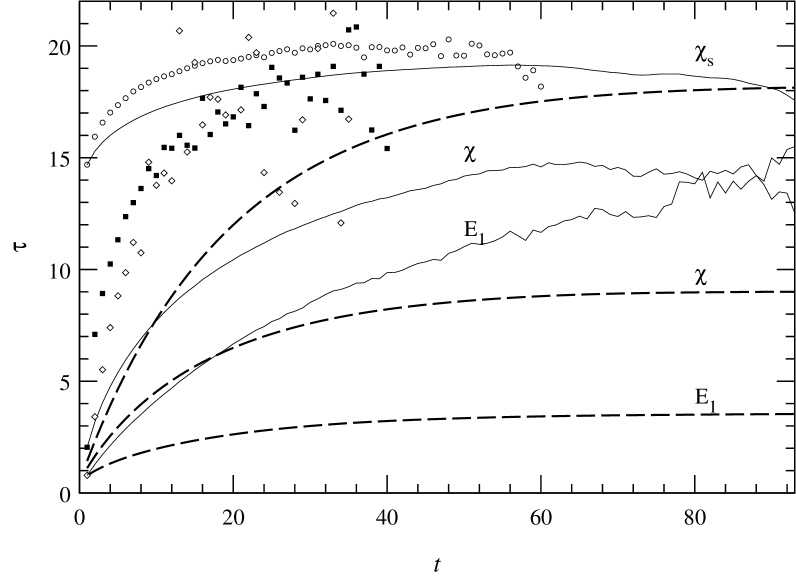
Figure 1: Autocorrelation time (in measures) estimators for $\chi_{\mathrm{s}}$, $\chi$ and $E_{1}$ in a $L=32$ lattice at $\beta=-2.41$. The dashed line correspond to the integrated time, the solid one to $\widehat{\tau}_{O}^{\mathrm{exp(1)}}$, and the symbols to $\widehat{\tau}_{O}^{\mathrm{exp(2)}}$ (circles, squares and diamonds for $\chi_{\mathrm{s}}$, $\chi$ and $E_{1}$, respectively).

A further check of statistical independence can be done by studying the errors computed with bins of data of increasing size. This could allow us to observe AT at scales much greater than the previous.

Figure 2: Statistical errors of $\chi_{\mathrm{s}}$ (upper curve) and $E_{1}$ (lower curve) as a function of the bin size (in measures) for $L=32$. The vertical dashed line corresponds to the bin size used in the analysis.

In fig. 2 we show the statistical errors for the energy and the staggered susceptibility in $L=32$ as a function of the length of the bins, using all the statistics. When their size is not big enough, the data in different bins are correlated and so, we see a growing error. When the size of the bins is enough to consider them independent, there is a plateau, that indicates the correct value for the statistical error. We can estimate the integrated AT from the quotient between the value of the error at large $L_{\mathrm{bin}}$ and at $L_{\mathrm{bin}}=1$, since $\sigma(L_{\mathrm{bin}})/\sigma(1)\to\sqrt{2\tau^{\mathrm{int}}}$. Using this procedure we obtain $\tau_{\chi_{\mathrm{s}}}^{\mathrm{int}}=172$ sweeps and $\tau_{E_{1}}^{\mathrm{int}}=34$ sweeps, in good agreement with the values shown in table 1.

From these figures we also observe that our choice of the number of bins, 50, is completely safe, allowing an accurate estimation of the statistical errors. We have chosen a large number of bins to ensure a 10% precision in the statistical error determination.

From our results we find very unlikely the existence of a much greater AT for any other important observables.

4 Measures of Critical Exponents.

Recalling that this model has two different order parameters (6,7) and, in principle, two different channels for the correlation lengths, it is compulsory to study separately both critical behaviors. Therefore, in addition to the usual exponents ($\nu$,$\beta$,$\gamma$ and $\eta$), we consider the analogous for the staggered channel ($\nu_{\mathrm{s}}$,$\beta_{\mathrm{s}}$,$\gamma_{\mathrm{s}}$ and $\eta_{\mathrm{s}}$). Although the most economic scenario requires $\nu=\nu_{\mathrm{s}}$, in order to consistently define a single continuous limit, we shall check this assumption.

4.1 Finite-size scaling.

Our measures of the critical exponents are based on the FSS ansatz. Let $\langle O(L,\beta)\rangle$ be the mean value of an operator $O$ measured on a size $L$ lattice, at a coupling value $\beta$, and let $\xi(L,\beta)$ be a reasonable estimator for the correlation length on a finite lattice, such as the one shown in eq. (11). Then, if $O(\infty,\beta)\sim|\beta-\beta_{\mathrm{c}}|^{-x_{O}}$, from the FSS ansatz one readily obtains [29]

$$\langle O(L,\beta)\rangle=L^{x_{O}/\nu}\left[F_{O}(\xi(L,\beta)/L)+L^{-\omega}G_{O}(\xi(L,\beta)/L)\right]+\ldots,$$ (26)

where $\omega$ is the universal exponent associated to the leading corrections-to-scaling. The dots stand for higher order scaling corrections and $\xi(\infty)^{-\omega}$ terms, negligible in the critical region. The above expression is straightforwardly generalized to functions of mean values.

We remark that to obtain eq. (26) the condition on the definition of the correlation length is that $\xi(L,\beta)/L$ should be a smooth monotonous function of $L/\xi(\infty,\beta)$ and that $x_{\xi}=\nu$. That condition is verified by the quantity defined in eq. (11) but also by $\kappa L$ (see eq. (10)) and their staggered counterparts. However, the scaling function $G_{O}$ is not invariant under a change of the correlation length definition, and a proper choice can largely reduce it.

Let us emphasize that the fulfillment of the hyperscaling relations is an a priory condition of the ansatz. In fact, if a relation like (26) holds, for example, for the magnetization and its square, one readily obtains $\gamma+2\beta=d\nu$. However, we will check the observance of the hyperscaling relations as a test of consistency.

4.2 Measuring at the maxima.

Usually, the application of FSS consists on measuring the mean value of an observable for different lattice sizes in the apparent critical point, where $L/\xi(L,\beta)$ is assumed to be constant, so the exponent of $L$ is easily extracted, after ensuring that the corrections-to-scaling are small. Typically one can define two such points, one is the infinite volume critical point (see section 5), the other is the peak of some quantity like the connected susceptibility defined as

$$\chi^{\mathrm{c}}=\chi-VM^{2}.$$ (27)

The advantage of measuring at a peak is that the apparent critical point is self defined, and also that the statistical error is much smaller at a peak (zero $\beta$ derivative) than when the slope is large.

In fig. 3 we plot the connected staggered susceptibility for several lattice sizes. The most significant property is the large shift of the apparent critical point, that makes necessary to perform simulations at values of the couplings dependent on the lattice size, as $\beta_{\mathrm{c}}$ cannot be reached with the spectral density method. The MC data used in fig. 3 correspond to short runs performed at the coupling values signed by filled symbols.

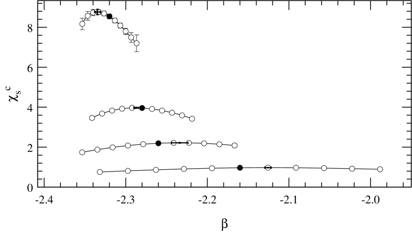
Figure 3: Connected staggered susceptibility as a function of lattice sizes (from top to bottom) $L=24,16,12,8$. The left limit of the $\beta$ axis corresponds to $\beta_{\mathrm{c}}$.

The shift of the $\beta$ value corresponding to the maximum of the staggered susceptibility, $\Delta\beta_{\mathrm{c}}^{L}$, can be used to measure the thermal exponent $\nu$ and the critical coupling in the thermodynamic limit. The expected behavior is $\Delta\beta_{\mathrm{c}}^{L}\propto L^{1/\nu}$. Performing a three parameters fit, we obtain for $L=8,12,16,24$: $\nu_{\mathrm{s}}=0.83(11)$, $\beta_{\mathrm{c}}=-2.410(22)$, with $\chi^{2}/\mathrm{d.o.f}=0.05/1$.

We can also compute $\eta_{\mathrm{s}}$ from the value of the susceptibility at the maximum. The fit gives $\eta_{\mathrm{s}}=0.035(39)$, with $\chi^{2}/\mathrm{d.o.f.}=0.98/1$. The value for $\eta_{\mathrm{s}}$ is compatible with those obtained below, but the errors are 30-times greater (the statistics used is 200-times smaller). This method has three important drawbacks compared with the methods discussed below: a) it is less precise; b) it needs simulations performed far from the critical point at a coupling value that depends on the observable to study; and c) large corrections-to-scaling are expected due to the large distance from the critical point.

Other quantities, as $\beta$ derivatives of magnetizations or correlation lengths also present peaks, but they are usually very broad and noisy what implies a low quality of the obtained critical exponents. The specific heat does not present a critical divergence as the $\alpha$ exponent is negative (see subsection 5.2).

4.3 The quotient method.

Fortunately, one can use another method that does not require a previous knowledge of the critical point, and which is directly based on eq. (26). Let $O$ be an observable whose mean value is measured at the same coupling in two lattices of sizes $L_{1}$ and $L_{2}$ respectively. Using (26) we can write for their quotient

$$Q_{O}=\frac{\langle O(L_{2},\beta)\rangle}{\langle O(L_{1},\beta)\rangle}=s^{x_{O}/\nu}\frac{F_{O}\left(\xi(L_{2},\beta)/L_{2}\right)}{F_{O}\left(\xi(L_{1},\beta)/L_{1}\right)}+O(L^{-\omega}),$$ (28)

where $s=L_{2}/L_{1}$. In the case of $O\equiv\xi$, the exponent $x_{\xi}$ is just $\nu$. Choosing the coupling in such a way that $Q_{\xi}=s$ we can directly compute the exponent for any operator as

$$\left.Q_{O}\right|_{Q_{\xi}=s}=s^{x_{O}/\nu}+O(L^{-\omega}).$$ (29)

As the exponents are obtained from just two independent simulations, it is possible to do a very clear statistical analysis. The use of the spectral density method avoids the necessity of an a priori knowledge of the coupling where the quotient of correlation lengths is the desired.

Figure 4: Quotient of staggered correlation lengths for $L_{2}/L_{1}=2$ as a function of $\xi_{\mathrm{s}}(L_{1})/L_{1}$ (upper side). In the middle we plot the same quantity for the staggered susceptibility. In both cases the higher line corresponds to $L_{1}=6$ with lattice sizes increasing with decreasing heights. Finally (lower side) $Q_{\chi_{\mathrm{s}}}$ as a function of $Q_{\xi_{\mathrm{s}}}$ for $L_{2}/L_{1}=2$ is plotted.

Let us show with an example how does it work. In fig. 4 (upper part) we plot the quotient between the staggered correlation lengths for $L_{2}/L_{1}=2$ as a function of the correlation length in the smaller lattice, in lattice size units. For $L_{1}$ large we should obtain a single curve. The deviations correspond to corrections-to-scaling. If we plot the quotient for the staggered susceptibility, we observe similar corrections-to-scaling (see fig. 4, middle part). Plotting $Q_{\chi_{\mathrm{s}}}$ as a function of $Q_{\xi_{\mathrm{s}}}$ the corrections-to-scaling are strongly reduced even for lattice sizes as small as $L_{1}=6$ (see fig. 4, lower part).

With this technique, we have studied several operators as the susceptibility ($x_{\chi}=\gamma$), the magnetization ($x_{M}=-\beta$) as well as their staggered counterparts. To compute the $\nu$ exponent, we use $\beta$ derivatives of observables. For example, $x_{\mathrm{d}\xi/\mathrm{d}\beta}=\nu+1$. In the next two subsections we shall separately study the determination of $\nu$ and $\eta$ type exponents.

4.3.1 The exponent $\nu$.

In the first two columns of table 2, we show the values obtained for the $\nu$ exponent measuring, at $Q_{\xi_{s}}=2$, the $\beta$ derivatives of $\xi_{\mathrm{s}}$ and $\xi$. The errors have been computed using the jack-knife method. The corrections-to-scaling are smaller than the statistical errors, even for lattice sizes as small as $L=6$.

We have repeated the analysis, using the non-staggered correlation length as the variable. In columns 3 and 4 we write down the obtained results. These are fully compatible with the previous, but with a slightly greater statistical error.

Table 2: $\nu$ exponent obtained from a FSS analysis using data from lattices of sizes $L$ and $2L$. In the first row we show the correlation length that we ask for duplicate, and in the second one the operator whose quotient we measure.

   $\xi_{\mathrm{s}}$ $\xi$ $\xi_{\mathrm{s}}$ $L$ $\!\mathrm{d}\xi_{\mathrm{s}}/\!\mathrm{d}\beta$ $\!\mathrm{d}\xi/\!\mathrm{d}\beta$ $\!\mathrm{d}\xi_{\mathrm{s}}/\!\mathrm{d}\beta$ $\!\mathrm{d}\xi/\!\mathrm{d}\beta$ $\!\!\!\!\mathrm{d}\log\!M_{\mathrm{s}}/\!\mathrm{d}\beta$ $\!\!\!\!\mathrm{d}\log\!M/\!\mathrm{d}\beta$ 6 .786(6) .790(6) .774(14) .759(16) .689(4) .670(4) 8 .785(4) .781(4) .771(7) .774(7) .717(3) .706(2) 12 .789(8) .782(9) .781(18) .781(15) .739(9) .731(8) 16 .786(6) .780(5) .782(8) .781(6) .755(4) .751(4) 24 .77(2) .77(2) .77(3) .77(2) .756(16) .758(13)   

Finally (columns 5 and 6 of table 2) we have alternatively computed the $\nu$ exponent using the logarithmic derivative of the magnetizations, which scales as $L^{1/\nu}$. The results have a smaller statistical error, but they suffer from important corrections-to-scaling, and it is necessary to compute the $L\to\infty$ extrapolation. This introduces uncertainties reducing the quality of these numbers as compared with the previous. Other quantities such as $\beta$-derivatives of Binder’s Cumulants suffer from statistical errors about three times larger, and therefore are quite useless for comparison.

We remark that all the determinations of the $\nu$ exponents (regardless the observables used being staggered or not) are compatible within errors (at the 1% level). One relevant question is whether summing data from different observables it is possible to reduce the statistical error, or even if the differences between columns are significant. As all the used quotients are flat functions of $Q_{\xi}$, the main contribution to the error is due to the observable (not to the correlation length). We have studied the mean and the difference of the first two columns. The reductions of the error bars in the first case are negligible (less than a 10%) because the data are strongly correlated. In the case of the difference, the correlation makes the error slightly smaller (about a 10%) than each term. The results do not show any significant deviation from zero.

The results for pairs with $s=3/2$ or $s=4/3$, that can be formed with the simulated lattice sizes, are compatible. As our better statistics are in the $L=16,32$ lattices, we only report the results for $s=2$.

4.3.2 $\eta$ exponents.

The $\eta$ exponent can be obtained from the scaling of the magnetization or of the susceptibility, using the scaling relations: $2\beta/\nu=d-2+\eta$ and $\gamma/\nu=2-\eta$.

The results for the $\eta_{\mathrm{s}}$ exponent are given in table 3. They have been obtained studying, in the staggered channel, the susceptibility, the magnetization and the maximum eigenvalue of the magnetization tensor (that scale with $\gamma_{\mathrm{s}}$, $\beta_{\mathrm{s}}$, and $\beta_{\mathrm{s}}$ respectively). Technically, the computation is somewhat different than in the case of the $\nu$ exponent, since the quotients change now very fast with $Q_{\xi_{\mathrm{s}}}$. One has to consider carefully the statistical correlation of the data. Thus we are able to measure $\gamma_{\mathrm{s}}/\nu$ with an accuracy of about a 0.1%, from which we can compute $\eta_{\mathrm{s}}=2-\gamma_{\mathrm{s}}/\nu$ with a 5% error.

For the non-staggered channel the results are reported in table 4. The columns 2, 3 and 4 correspond to the use of $Q_{\xi_{\mathrm{s}}}$ as the variable. We observe important corrections-to-scaling. The use of $Q_{\xi}$ does not improve the results. Using $Q_{\kappa L}$, we find a quite strong reduction of the corrections-to-scaling.

Table 3: $\eta_{\mathrm{s}}$ exponent obtained from the FSS of the staggered susceptibility, magnetization and maximum eigenvalue of the magnetization, using $\xi_{\mathrm{s}}$ as the variable. In all cases, the pairs are of type $(L,2L)$.

   $L$ $\chi_{\mathrm{s}}$ $M_{\mathrm{s}}$ $\lambda_{\mathrm{s}}^{\mathrm{max}}$ 6 0.0431(10) 0.0474(9) 0.0480(12) 8 0.0375(7) 0.0409(8) 0.0409(9) 12 0.0357(17) 0.0382(18) 0.039(2) 16 0.0375(12) 0.0395(12) 0.0395(13) 24 0.038(5) 0.038(5) 0.035(6)   

Table 4: $\eta$ exponent obtained from the susceptibility, magnetization and maximum eigenvalue of the magnetization in $(L,2L)$ lattices. In the first row we indicate the quantity used as the variable.

   $\xi_{\mathrm{s}}$ $\kappa L$ $L$ $\chi$ $M$ $\lambda^{\mathrm{max}}$ $\chi$ $M$ $\lambda^{\mathrm{max}}$ 6 1.442(2) 1.447(2) 1.442(3) 1.332(6) 1.332(6) 1.332(5) 8 1.413(2) 1.416(2) 1.4135(18) 1.332(4) 1.332(4) 1.334(4) 12 1.391(3) 1.393(3) 1.396(4) 1.320(13) 1.321(13) 1.327(12) 16 1.381(3) 1.383(3) 1.384(3) 1.339(5) 1.340(5) 1.343(5) 24 1.362(8) 1.365(9) 1.362(10) 1.334(18) 1.334(18) 1.332(17)   

5 Corrections to scaling.

For the determination of the corrections-to-scaling exponent, $\omega$, we have used the property shared by different observables (Binder type parameters, $\kappa$, and correlation lengths divided by the lattice size) that asymptotically should cross at the critical point. It can be shown [20] that the scaling functions corresponding to lattice sizes $L_{1},L_{2}$ cross at a $\beta$ value whose shift from the critical value behaves as

$$\Delta\beta^{L_{1},L_{2}}\propto\frac{1-s^{-\omega}}{s^{\frac{1}{\nu}}-1}L_{1}^{-\omega-\frac{1}{\nu}},$$ (30)

where $s=L_{2}/L_{1}$. In fig. 5 we plot the values of the coupling where several scaling functions cross, as a function of $L_{2}^{-1/\nu}$. We use along this subsection the value $\nu=0.783$. According to (30) if we fix $L_{1}$, the asymptotic behavior should be linear, what is well satisfied in the plot.

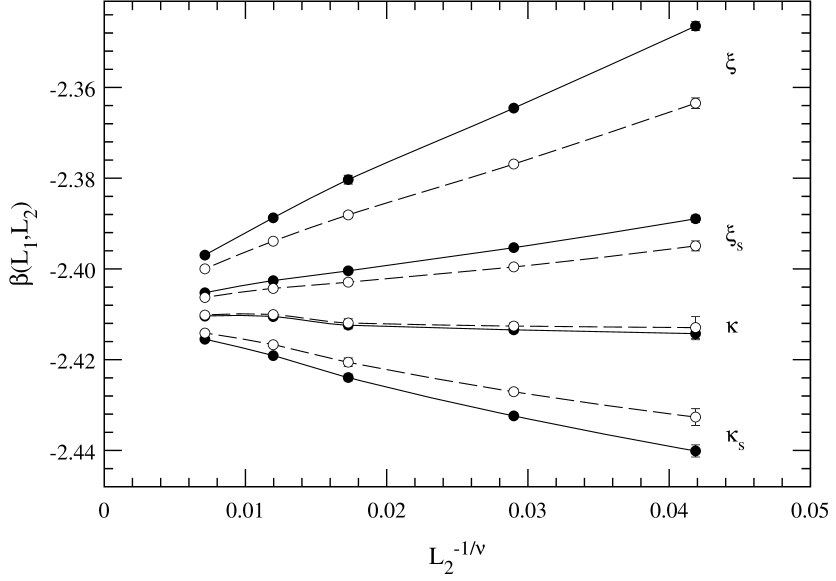
Figure 5: Crossing points of scaling functions for pairs $(L_{1},L_{2})$, as a function of $L_{2}^{-1/\nu}$, for $L_{1}=6$ (solid lines) and $L_{1}=8$ (dashed line), and $L_{2}=12,16,24,32,48$.

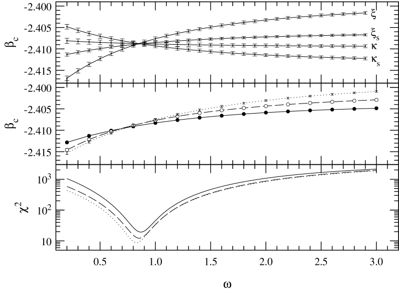
Figure 6: Critical coupling extrapolated from the intersection with $L_{1}=6$ for $\kappa$, $\kappa_{\mathrm{s}}$, $\xi/L$ and $\xi_{\mathrm{s}}/L$ as a function of the $\omega$ exponent (upper part). Fits to a single $\beta_{\mathrm{c}}$ value for $L_{1}=6$ (solid line), $L_{1}=8$ (dashed line), and $L_{2}/L_{1}=2$ (dotted line) as a function of $\omega$ (middle). In the lower side we show the values of $\chi^{2}$ for the latter fits.

We have performed a global fit of the points from each observable to a functional dependence of the type of eq. (30) with $L_{1}=6$. The good precision obtained for the $\nu$ exponent makes negligible the uncertainty that comes from this quantity. In fig. 6 (upper part) we plot the values of the extrapolated $\beta_{\mathrm{c}}$ from independent fits for every observable after fixing the value of the corrections-to-scaling exponent $\omega$.

Studying the variation of the $\chi^{2}$ function (using the full covariance matrix) we obtain

$$\begin{array}[]{lll}\kappa_{\mathrm{s}}:&\beta_{\mathrm{c}}=-2.4097(19),&\omega=1.05(45),\\ \xi/L:&\beta_{\mathrm{c}}=-2.4096(23),&\omega=0.75(20),\\ \xi_{\mathrm{s}}/L:&\beta_{\mathrm{c}}=-2.4082(13),&\omega\in(0.6,1.9).\end{array}$$ (31)

The corrections-to-scaling in the $\kappa$ case are so small that it is not possible to measure the parameters. Repeating the fits with $L_{1}=8$ we obtain very similar results.

From these fits we conclude that all the extrapolated values coincide up to $\Delta\beta=0.002$. Notice that this implies that both correlation lengths diverge at values of $\beta$ which are at most $0.002$ apart. We can go one step further under the hypothesis that the extrapolated values must be the same, which imply that the infinite volume propagator has two separated poles in momentum space, one at the origin, the other at $(\pi/a,\pi/a,\pi/a)$. A $\chi^{2}$ minimization of all the (strongly correlated) data gives (see fig. 6, middle and lower parts)

$$\beta_{\mathrm{c}}=-2.4088(3),\omega=0.87(3),\chi^{2}/\mathrm{d.o.f.}=19.3/14.$$ (32)

We have repeated the fits discarding the $L_{1}=6$ data, and measuring the crossing with the $L_{1}=8$ curves. We obtain

$$\beta_{\mathrm{c}}=-2.4085(3),\omega=0.86(4),\chi^{2}/\mathrm{d.o.f.}=12.2/14,$$ (33)

that are fully compatible with a very slight increase of the statistical errors. This gives us confidence in the smallness of the higher order corrections-to-scaling.

A further check can be done studying the crossing between lattice sizes with $s=2$. The functional form of the fit is different now, as $s$ in eq. (30) is fixed. We obtain, discarding the $L=6$ data,

$$\beta_{\mathrm{c}}=-2.4087(4),\omega^{*}=0.83(4),\chi^{2}/\mathrm{d.o.f.}=8.7/10.$$ (34)

where $\omega^{*}$ is defined as $\omega+\frac{1}{\nu}-(0.783)^{-1}$.

We will use in the next subsection these results to study the infinite volume extrapolation of the critical exponents. On the other hand, with our $\beta_{\mathrm{c}}$ estimation, we can use again eq. (26) to obtain another estimation of critical exponents. This shall be done in subsection 5.2.

5.1 The infinite volume extrapolation of the exponents.

The FSS analysis has the nice feature of using the finite-size effects to measure quantities as important as critical exponents. However, this does not guarantee the absence of systematic errors coming from finite-size effects, that appear as corrections-to-scaling terms.

Let $x$ be the critical exponent under study, and let us suppose that we need to take care of just the first term on the corrections-to-scaling series, then we have from eq. (29),

$$\left.{\frac{x}{\nu}}\right|_{(2L,L)}=\frac{x}{\nu}+aL^{-\omega}+\ldots,$$ (35)

$a$ being a constant.

We have carried out a fit, to the above functional form, for the numbers obtained in subsections 4.3.1 and 4.3.2. We exclude the $L=6$ data, and take for the universal exponent $\omega$ the value obtained previously ($\omega=0.85(4)$).

We have found two very different situations. Some estimators present a non measurable size dependence (first four columns of table 2, the whole table 3, and the last three columns in table 4). For them, we find no dependence on $\omega$ (when it moves within its error bars) of the extrapolated exponent, that has a value almost equal to the most relevant number in the tables (the $L_{1}=16$, $L_{2}=32$ pair), but the errors are doubled.

We also have found estimators with a quite measurable size dependence, namely the last two columns of table 2 (exponent $\nu$), and the first three columns of table 4 (exponent $\eta$). The extrapolated values are

$$\begin{array}[]{c}\nu_{5}=0.800(9),\ \nu_{6}=0.804(8),\\ \eta_{1}=1.338(6),\ \eta_{2}=1.339(6),\ \eta_{3}=1.346(6),\end{array}$$ (36)

where the subindices refer to columns in tables 2 and 4. We find here an $\omega$-dependence of the extrapolated exponents of one half of the quoted statistical error. While the extrapolation for the $\eta$ exponent is fully consistent with the quoted numbers in the last three columns of table 4, the $\nu$ we get looks too big. Although both estimations are within two standard deviations, higher order corrections-to-scaling are apparent by plotting the last columns of table 2 as a function of $L^{-\omega}$.

As a final result for the exponents, we choose operators that give stable values with the lattice size, taking the measure for the $(16,32)$ pair; the number in the second parenthesis shows the error increase due to the extrapolation that can be taken as an estimation of the error involved in this procedure:

$$\begin{array}[]{lcllcllll}\nu&=&0.783(5)(6),\\ \eta_{\mathrm{s}}&=&0.0380(12)(14),&\quad(\beta_{\mathrm{s}}&=&0.406(3)(3),\ \gamma_{\mathrm{s}}&=&1.536(10)(12)&),\\ \eta&=&1.339(5)(5)&\quad(\beta&=&0.916(6)(7),\ \gamma&=&0.518(6)(7)&).\end{array}$$ (37)

For comparison, we quote the MC results for $\nu$ obtained for the three dimensional ferromagnetic $\mathrm{O}(3)$ [30] and $\mathrm{O}(4)$ [18] models:

$$\begin{array}[]{rcl}\nu(\mathrm{O}(3))&=&0.704(6),\\ \nu(\mathrm{O}(4))&=&0.7479(90).\end{array}$$ (38)

Our results for the $\mathbf{R}\mathrm{P}^{2}$ model are completely incompatible to those of the $\mathrm{O}(3)$ one. Regarding the $\mathrm{O}(4)$ model, although the differences are small, the value for the $\nu$ exponent seems also incompatible.

5.2 Critical exponents measuring at ${\mathbf{\beta_{\mathrm{c}}}}$.

Taking the values $\beta_{\mathrm{c}}=-2.4086(4)$ and $\omega=0.85(4)$ we will repeat the measurements of the critical exponents using the measures of the usual operators at a fixed coupling. As in the determination of $\beta_{\mathrm{c}}$ we use all the MC data, it is difficult to perform a correct computation of the statistical errors taking into account all correlations. In addition, there are several sources of systematic errors, consequently the evaluation of the errors on the exponent is harder.

The functional form we fit is $AL^{x/\nu}(1+bL^{-\omega})$, where $\omega$ is fixed. We present the results for the computed exponents in table 5. In the first column we show the minimum value of $L$ that we include in the fit. We remark that the inclusion of the $L^{-\omega}$ term is essential to get a correct fit. To estimate the errors, we have extrapolated at our measured $\beta_{\mathrm{c}}$ and at one standard deviation, adding the difference to the statistical error in the extrapolation. The $\omega$ error contribution is negligible.

Table 5: Critical exponents obtained by measuring at $\beta_{\mathrm{c}}$. $L$ stands for the minimum value of the lattice size we have used for the fit. The contribution of the error in $\beta_{\mathrm{c}}$ and $\omega$ is included.

   $\nu$ $\eta_{\mathrm{s}}$ $\eta$ $L$ $d\xi_{\mathrm{s}}/d\beta$ $d\xi/d\beta$ $\chi_{\mathrm{s}}$ $M_{\mathrm{s}}$ $\chi$ $M$ 6 0.783(9) 0.761(9) 0.030(7) 0.030(7) 1.324(12) 1.323(13) 8 0.784(15) 0.771(14) 0.023(9) 0.023(10) 1.316(16) 1.316(16) 12 0.79(3) 0.79(3) 0.011(16) 0.010(17) 1.292(27) 1.291(27) 16 0.75(7) 0.82(8) 0.02(3) 0.02(3) 1.31(5) 1.31(5)   

For the $\eta$ exponents, as the slope of $M$ and $\chi$ as a function of $\beta$ is large at the critical point, the errors in the determination of $\beta_{\mathrm{c}}$ affect strongly that of $\eta$. This error is, in part, overestimated since we do not take into account the statistical correlation between the measures used to determine $\beta_{\mathrm{c}}$ and the magnetization operators. This, albeit complex, could have been done. However, as the $\beta_{\mathrm{c}}$ value has been obtained after a somewhat elaborated procedure, the influence of systematic errors is difficult to quantify. Consequently we consider more solid the determination obtained from the quotient method.

From the hyperscaling relation $\alpha=2-d\nu$, using (37), we have $\alpha/\nu=-0.44(2)$ and therefore, no divergence is to be seen for the specific heat. We could nevertheless stick to the FSS prediction. In fact in fig. 7 we show the specific heat at the critical point as a function of $L^{\alpha/\nu}$. Strong scaling corrections are apparent, but the overall linear behavior is well satisfied.

Figure 7: Specific heat at the critical point for all lattice sizes as a function of $L^{\alpha/\nu}$. The linear fit has been done for $L\geq 16$

6 Vacuum structure in the critical region.

The antiferromagnetic broken phase is characterized by a $L\to\infty$ nonzero value for the magnetizations $M$ and $M_{\mathrm{s}}$. However, studying the different terms of the tensors we can obtain a lot of information about the structure of the broken phase. We shall consider the behavior of several operators constructed from the magnetization tensors. As the staggered magnetization behaves as $t^{\beta_{\mathrm{s}}}$ ($\beta_{\mathrm{s}}\sim 0.4$) and the magnetization as $t^{\beta}$ ($\beta\sim 0.9$) the former is dominant for $t$ small, $t$ being the reduced temperature.

The first question we address is the breakdown of the even-odd symmetry. Near to the critical point it is very difficult to reach an asymptotic ($L\to\infty$) behavior that allows us to know if that symmetry is broken, but instead we can use FSS arguments to find the answer.

Let us consider the tensors product trace

$$\mathop{\mathrm{tr}}\mathbf{M}_{\mathrm{s}}\mathbf{M}=\frac{1}{4}(\mathop{\mathrm{tr}}\mathbf{M}^{2}_{\mathrm{e}}-\mathop{\mathrm{tr}}\mathbf{M}^{2}_{\mathrm{o}}),$$ (39)

where $\mathbf{M}_{\mathrm{e}}=2/V\sum_{i\ \mathrm{even}}\mathbf{T}_{i}$ and analogously for the odd sublattice. If the even-odd symmetry were not broken, the $\mathbf{M}_{\mathrm{s}}\mathbf{M}$ tensor should go to zero as $1/V=L^{-3}$, while the LHS of eq. (39) is bounded by a $L^{-(\beta_{\mathrm{s}}+\beta)/\nu}$ behavior. In practice we have studied the quantity $A=\langle(\mathop{\mathrm{tr}}\mathbf{M}_{\mathrm{s}}\mathbf{M})^{2}\rangle$.

We have used again the technique described in subsection 4.3 to determine the critical exponent. We obtain, after an $L\to\infty$ extrapolation the value

$$\frac{x_{A}}{\nu}=-3.389(15),$$ (40)

which is compatible with $-2(\beta+\beta_{\mathrm{s}})/\nu=-3.377(13)$, and discards the $-6$ value. We thus conclude that the even-odd symmetry breakdown does occur.

The naive picture that comes from the previous conclusion is that one of the sublattices is plane aligned and the other fully aligned, and the $\mathrm{O}(2)$ global symmetry is preserved. To check this we have studied the conmutator of the $\mathbf{M}_{\mathrm{s}}$ and $\mathbf{M}$ tensors. If there were a remaining $\mathrm{O}(2)$ symmetry, both tensors could be simultaneously diagonalized and the conmutator should vanish. In a finite lattice, according to FSS it should behave as $L^{-d/2-\beta_{\mathrm{s}}/\nu}$. Our results show that the exponent for $B=\langle\mathop{\mathrm{tr}}[\mathbf{M}_{\mathrm{s}},\mathbf{M}][\mathbf{M}_{\mathrm{s}},\mathbf{M}]^{\dagger}\rangle$ has strong corrections-to-scaling, but after a $L\to\infty$ extrapolation we obtain

$$\frac{x_{B}}{\nu}=-3.406(11).$$ (41)

Due to these corrections the error bar is probably underestimated. We observe that is again very different from $-4.04(2)$ and compatible with $-2(\beta+\beta_{\mathrm{s}})/\nu$. The consequences of these results are that the $\mathrm{O}(2)$ symmetry must be broken, and that the alignment directions of both sublattices are not orthogonal.

7 Numerical results at low temperature.

We present in this section some numerical results obtained from simulations in the low temperature ($\beta<\beta_{\mathrm{c}}$) region. The very first thing to establish is the existence of a low temperature phase, where both order parameters are not zero, and where the symmetry between the even and odd sublattices is broken, as discussed in the previous section. We can answer both questions computing an histogram of $\mathop{\mathrm{tr}}(\mathbf{M}\mathbf{M}_{\mathrm{s}})$. This is shown in fig. 8 for $\beta=-3.0$. We see a clearly nonzero thermodynamic limit for $\mathop{\mathrm{tr}}(\mathbf{M}\mathbf{M}_{\mathrm{s}})$. For $\beta<-3$, the double peak structure is even clearer.

Figure 8: Histogram of $\mathop{\mathrm{tr}}\mathbf{M}_{\mathrm{e}}^{2}-\mathop{\mathrm{tr}}\mathbf{M}_{\mathrm{o}}^{2}$ at $\beta=-3.0$ for several lattice sizes.

Figure 9: Histogram of the next-nearest neighbors energy for the even and odd sublattices. The dashed line corresponds to the effective (flat) low temperature model for $L=16$.

We have next studied the second-neighbor energy for the odd and even sublattices independently. In fig. 9 we plot the histograms of the sublattice energy. We recall that for $\beta=-\infty$, $E_{2}=1$ for one of the sublattices and $E_{2}=0.5$ for the other. We observe a clear double peak structure at $\beta=-4$ (upper side). At $\beta=-10$ (lower side) the double peak structure is already clear even for lattice sizes as small as $L=4$ and for $L\geq 8$ the peaks are completely split. The dotted line corresponds to the flat model (subsection 2.5), this means that for this $\beta$ value the results are almost asymptotic ($\beta\to-\infty$) for the left peak.

It is very interesting to observe the evolution of the second-neighbor energy for the less aligned sublattice. At $-\beta$ very large, the field variables are almost in a S¹ subset of S², so, we can look at it as an $\mathbf{R}\mathrm{P}^{1}$ model in a face centered cubic (fcc) lattice. This model (that is equivalent to an $\mathrm{O}(2)$ sigma model) has a second order phase transition. For a rough comparison we have measured the energy $\langle\cos^{2}(\varphi_{i}-\varphi_{j})\rangle$ for the fcc $\mathbf{R}\mathrm{P}^{1}$ model at the critical point, obtaining $E_{2}=0.62(1)$.

In the $\mathbf{R}\mathrm{P}^{2}$ model, the fluctuations produce an effective coupling between second-neighbors of the less aligned sublattice. For $-\beta$ very large, we can use the flat model defined by (20). We obtain $E_{2}\approx 0.53$ for the less aligned sublattice (see fig. 9). This value is very small, so the effective coupling is too weak to produce an $\mathrm{O}(2)$ ordering.

For increasing values of $\beta$, the fluctuations off the plane reduce the $E_{2}$ value although $\langle\cos^{2}(\varphi_{i}-\varphi_{j})\rangle$ increases. This effect can be taken into account in a crude approximation as follows. Let us write the spin variable as in eq. (19). The second-neighbor energy takes the form

$$\begin{array}[]{rcl}\langle(\mbox{\boldmath$v$}_{i}\cdot\mbox{\boldmath$v$}_{j})^{2}\rangle&=&\langle(1-(v_{i}^{z})^{2})(1-(v_{j}^{z})^{2})\cos^{2}(\varphi_{i}-\varphi_{j})\rangle+\langle(v_{i}^{z}v_{j}^{z})^{2}\rangle\\ &&+\langle v_{i}^{z}v_{j}^{z}\sqrt{1-(v_{i}^{z})^{2}}\sqrt{1-(v_{j}^{z})^{2}}\cos(\varphi_{i}-\varphi_{j})\rangle.\end{array}$$ (42)

As a first approximation, we can suppose that the $z$ components of the neighbors are uncorrelated, and similarly for the $z$ components with the angles. Thus we can factorize the mean values obtaining

$$E^{\mathbf{R}\mathrm{P}^{1}}\equiv\langle\cos^{2}(\varphi_{i}-\varphi_{j})\rangle\approx\frac{E_{2}-\lambda_{\mathrm{min}}^{2}}{(1-\lambda_{\mathrm{min}})^{2}},$$ (43)

where $\lambda_{\mathrm{min}}=\langle(v_{i}^{z})^{2}\rangle$ is the minimal eigenvalue of the magnetization tensor of the less aligned sublattice.

The numerical results obtained for several $\beta$ values are

$$\begin{array}[]{ll}\beta=-10,&E^{\mathbf{R}\mathrm{P}^{1}}=0.53(1),\\ \beta=-4,&E^{\mathbf{R}\mathrm{P}^{1}}=0.61(1),\\ \beta=-3,&E^{\mathbf{R}\mathrm{P}^{1}}=0.65(1),\\ \beta=-2.41,&E^{\mathbf{R}\mathrm{P}^{1}}=0.798(2).\end{array}$$ (44)

We observe a fast increase of that quantity when approaching to the critical point. In particular, the critical value for the $\mathrm{O}(2)$ model is reached at $\beta=-4.0$. This argument, although qualitative, supports the idea that the breakdown of the $\mathrm{O}(2)$ symmetry observed at the critical point can be explained with the induced interaction of the more ordered sublattice on the less ordered one.

We expect that the breakdown of the $\mathrm{O}(2)$ symmetry occurs at $\beta<\beta_{\mathrm{c}}$ since $E^{\mathbf{R}\mathrm{P}^{1}}$ becomes very large at $\beta_{\mathrm{c}}$. However, we have been unable to obtain a clear thermodynamic limit at $\beta<\beta_{\mathrm{c}}$ for an $\mathrm{O}(2)$ broken phase. Let us state that for an $\mathrm{O}(2)$ symmetric phase, we expect to find a diminishing difference of the two smaller eigenvalues of the global magnetization as $L^{-\frac{d}{2}}$. In fig. 10, we plot this difference as a function of $L^{-\frac{d}{2}}$, for two $\beta$ values. At $\beta=-4$, the analysis for $L\leq 32$ lattices shows an $\mathrm{O}(2)$ symmetric thermodynamic limit. At $\beta=-3$, the same analysis seems to indicate an $\mathrm{O}(2)$ non-symmetric behavior for $L\leq 32$, but the $L=48$ data points to a restoration of the symmetry. Finding a clear non symmetric limit would imply to simulate nearer to $\beta_{\mathrm{c}}$ in much larger lattices than those we have used in this work.

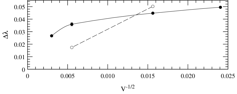
Figure 10: Difference of the two smaller eigenvalues of $\mathbf{M}$ as a function of $V^{-\frac{1}{2}}$ for $L=16,32$ at $\beta=-4.0$ (dashed line), and for $L=12,16,32,48$ at $\beta=-3.0$ (solid line).

There is an alternative procedure that we think easier and more conclusive that consists in the introduction of a second-neighbor coupling which explicitly breaks the $\mathrm{O}(2)$ symmetry

$$\mathcal{S}_{2}=\beta_{2}\sum_{\ll i,j\gg}(\mbox{\boldmath$v$}_{i}\cdot\mbox{\boldmath$v$}_{j})^{2}.$$ (45)

Let us discuss some regions of the $(\beta,\beta_{2})$ plane. For $\beta=-\infty$, the line $\beta_{2}$ corresponds to a fcc $\mathbf{R}\mathrm{P}^{1}$ ($\equiv\mathrm{O}(2)$) model that presents a second-order phase transition at $\beta_{2}=0.415(1)$. At $-\beta$ large but finite, we expect a second order line, in the same universality class, almost parallel to the $\beta$ axis. As the fluctuations of the more aligned sublattice help in the $\mathrm{O}(2)$ ordering, this line should get closer to the $\beta$ axis and presumably crosses it before $\beta_{\mathrm{c}}$. We project to study this enlarged parameter space shortly.

8 Conclusions and outlook.

We have found very interesting properties in the AF sector of the $\mathbf{R}\mathrm{P}^{2}$ spin model in three dimensions. It presents two magnetization operators with different critical properties, what is related with an odd property of the vacuum in the critical region: a complete breakdown of the global $\mathrm{O}(3)$ symmetry of the action. We have accurately measured the critical exponents, using a modest amount of computer time, by means of a FSS method that performs very good even in the presence of important corrections-to-scaling. The critical exponents obtained are clearly different from those of the ferromagnetic $\mathrm{O}(3)$ model, and hardly compatible with the ones reported for $\mathrm{O}(4)$.

We project to extend these results to several related models, with generalizations such as, for instance, the inclusion of second-neighbor interactions or of vectorial interactions. Work is already in progress [31] on the four dimensional version of this model. We are particularly interested in the relevance, in $d=4$, of the properties found here. In addition, it can enlighten the mechanism by which the AF transition seems to belong to a new Universality Class in $d=3$.

Appendix A Details of the Mean-Field computation.

To compute the function ${\mathcal{G}}_{\rho}$ defined in (15) we start from the Hamiltonians written in terms of the tensorial products $\mbox{\boldmath$\tau$}_{i}=\mbox{\boldmath$v$}_{i}\otimes\mbox{\boldmath$v$}_{i}$,

$${\mathcal{H}}=\sum_{<i,j>}\mathop{\mathrm{tr}}\mbox{\boldmath$\tau$}_{i}\mbox{\boldmath$\tau$}_{j},\\$$ (46)

$${\mathcal{H}}_{\rho}=-\sum_{i\ \mathrm{even}}\mathop{\mathrm{tr}}\mbox{\boldmath$\tau$}_{i}\mathbf{Q}_{\mathrm{e}}-\sum_{i\ \mathrm{odd}}\mathop{\mathrm{tr}}\mbox{\boldmath$\tau$}_{i}\mathbf{Q}_{\mathrm{o}},$$ (47)

where, given the antiferromagnetic character of our model, it is rather natural to use a (tensorial) mean field for the odd sublattice, and an independent one for the even sites. In this approximation the partition function factorizes as

$${\mathcal{Z}}_{\rho}=z_{\mathrm{e}}^{V/2}z_{\mathrm{o}}^{V/2},\quad z_{\mathrm{e,o}}=\int_{\mathrm{S}^{2}}\mathrm{d}\mbox{\boldmath$v$}\exp(\frac{1}{T}\mathop{\mathrm{tr}}\mbox{\boldmath$\tau$}\mathbf{Q}_{\mathrm{e,o}}),$$ (48)

and the mean value of $\tau$ can be written as

$$\langle\mbox{\boldmath$\tau$}_{\mathrm{e,o}}\rangle_{\rho}=\mathbf{M}_{\mathrm{e},o}(\mbox{\boldmath$Q$}_{\mathrm{e},o})=(z_{\mathrm{e,o}})^{-1}\int_{\mathrm{S}^{2}}\mathrm{d}\mbox{\boldmath$v$}\ \mbox{\boldmath$\tau$}\exp(\frac{1}{T}\mathop{\mathrm{tr}}\mbox{\boldmath$\tau$}\mathbf{Q}_{\mathrm{e,o}}).$$ (49)

We thus obtain the quantity to minimize, $\mathcal{G}_{\rho}$, as a function of $\mbox{\boldmath$Q$}_{\mathrm{e}},\mbox{\boldmath$Q$}_{\mathrm{o}}$, and the temperature $T$,

$$\frac{2}{V}{\mathcal{G}}_{\rho}=-T\log(z_{\mathrm{e}}z_{\mathrm{o}})-2d\,\mathop{\mathrm{tr}}\mathbf{M}_{\mathrm{e}}\mathbf{M}_{\mathrm{o}}+\mathop{\mathrm{tr}}\mathbf{M_{\mathrm{e}}Q_{\mathrm{e}}}+\mathop{\mathrm{tr}}\mathbf{M_{\mathrm{o}}Q_{\mathrm{o}}}.$$ (50)

It is easy to show that ${\mathcal{G}}_{\rho}$ is invariant if we add to $\mathbf{Q}_{\mathrm{e}}$ ($\mathbf{Q}_{\mathrm{o}}$) an arbitrary multiple of the identity. Thus, we can shift to zero, for each field, one of its eigenvalues.

Minimizing general tensorial fields would be very complex, so we shall restrict ourselves to the case $[\mathbf{Q}_{\mathrm{e}},\mathbf{Q}_{\mathrm{o}}]=0$, where they can be simultaneously diagonalized. From now on, we shall work in a basis where both fields are diagonal. Let us remark that an $\mathrm{O}(2)$-symmetric vacuum or a non-symmetric one, can be considered in this class. We shall write $\mathbf{Q}_{\mathrm{e}}$, ($\mathbf{Q}_{\mathrm{o}}$) as the diagonal matrix with eigenvalues $(q_{1},q_{2},0)$ ($(q_{3},q_{4},0)$). Consequently, $\mathbf{M}_{\mathrm{e,o}}$ are trace-one diagonal matrices, with nonnegative eigenvalues.

The values of the $q_{i}$ parameters that minimize $\mathcal{G}_{\rho}$ satisfy the equations

$$0=\mathop{\mathrm{tr}}\left((2d\/\mathbf{M}_{\mathrm{e}}-\mathbf{Q}_{\mathrm{o}})\frac{\partial\mathbf{M}_{\mathrm{o}}}{\partial q_{i}}\right),\ i=1,2,$$ (51)

and analogously for $i=3,4$ interchanging odd by even.

It is easy to check that $\mathbf{Q}_{\mathrm{e,o}}=0$ is a solution of (51) for all values of $T$. Nevertheless, this could correspond to a maximum as well as to a minimum of ${\mathcal{G}}_{\rho}$. In fact, one would expect this to be the minimum for large $T$, which would turn into a maximum for $T$ small enough.

Eqs. (51) are a set of quite complex nonlinear coupled equations. To go further, let us assume that the system undergoes a continuous transition at a critical point $T_{\mathrm{c}}$. We can thus linearize them as $0=\sum_{i=1}^{4}A_{ji}(T)q_{i}$, in order to find a minimum close to $\mathbf{Q}_{\mathrm{e,o}}=0$. To have a non trivial solution, we require $\det A(T)=0$, which happens at

$$\beta_{\mathrm{c}}=-\frac{1}{T}=-\frac{15}{4d}\ .$$ (52)

This nontrivial minima should be in the directions in $q$-space pointed by the vectors belonging to the kernel of the matrix $A$, that is spanned by the vectors $(1,0,-1,0)$ and $(0,1,0-1)$. We shall then restrict ourselves to the subspace $q_{1}=-q_{3}$, $q_{2}=-q_{4}$. Notice that there are three directions in this plane, where the ordered phase keeps an $\mathrm{O}(2)$ symmetry: $(1,1,-1,-1)$, $(1,0,-1,0)$, and $(0,1,0,-1)$. Expanding eq. (49) in powers of $q_{i}$ it is straightforward to see that the linear terms are opposite for $\mathbf{M}_{\mathrm{e}}$ and $\mathbf{M}_{\mathrm{o}}$ in this subspace, so, at first nonzero order

$$\begin{array}[]{cclcl}\mathbf{M}_{\mathrm{s}}&=&\frac{1}{2}(\mathbf{M}_{\mathrm{e}}-\mathbf{M}_{\mathrm{o}})&\propto&q_{i},\\ \mathbf{M}&=&\frac{1}{2}(\mathbf{M}_{\mathrm{e}}+\mathbf{M}_{\mathrm{o}})-\frac{1}{3}\mathbf{1}&\propto&q_{i}^{2},\\ E-\frac{1}{9}&=&\mathop{\mathrm{tr}}\mathbf{M}_{\mathrm{e}}\mathbf{M}_{\mathrm{o}}-\frac{1}{9}&\propto&q_{i}^{2}.\end{array}$$ (53)

To calculate the dependence of $q_{i}$ on $T$ we need to consider higher order terms in ${\mathcal{G}}_{\rho}$. We obtain, using polar coordinates in the $(q_{1},q_{2})$ plane

$${\mathcal{G}}_{\rho}=a+b(T-T_{\mathrm{c}})s^{2}+c(T)s^{4}+O(s^{6}),$$ (54)

where $s=r\sqrt{2-\sin 2\theta}$, and $b,c(T)>0$. At leading order we also find $\mathop{\mathrm{tr}}\mathbf{M}_{\mathrm{s}}^{2}\propto s^{2}$. For $T>T_{\mathrm{c}}$, $s=0$ is a minimum of ${\mathcal{G}}_{\rho}$, while when $T<T_{\mathrm{c}}$, $s=0$ is a maximum and the real minimum is at $s_{\mathrm{min}}\propto(T_{\mathrm{c}}-T)^{1/2}$. Therefore, the mean field prediction for the magnetic and specific heat critical exponents is

$$\beta_{\mathrm{s}}=1/2,\quad\beta=1,\quad\alpha=0.$$ (55)

Up to this order, the symmetry of the ordered phase cannot be determined since there are minima for $\mathcal{G}_{\rho}$ along all directions in the $(q_{1},q_{2})$ plane. The sixth order term does break this degeneracy but favors an $\mathrm{O}(2)$ symmetric ordered phase. This is in contradiction with our numerical data just after the transition.

Appendix B Classical continuum limit.

We shall derive the naive classical continuum limit for the $\mathbf{R}\mathrm{P}^{2}$ antiferromagnetic model. As we are interested in an $\mathrm{O}(2)$ broken phase, for consistency we should add to the action (1) a ferromagnetic second-neighbor term that, as we shall see, does not change the continuum functional form.

Let us first state that any integral over the S² sphere can be written as an integral over the $\mathrm{SO}(3)$ group. If $u$ is an arbitrary element of S², for any function $f$,

$$\int_{\mathrm{S}^{2}}\mathrm{d}\mbox{\boldmath$v$}f(\mbox{\boldmath$v$})=\int_{\mathrm{SO}(3)}\mathrm{d}Rf(R\mbox{\boldmath$u$}),$$ (56)

where $\mathrm{d}\mbox{\boldmath$v$}$ is the invariant measure over the sphere and $\mathrm{d}R$ the Haar measure over the $\mathrm{SO}(3)$ group, both normalized. This result is easily generalized to a multiple integral. In particular the partition function can be expressed as

$${\mathcal{Z}}\equiv\int_{S^{2}}\left(\prod_{i}\mathrm{d}\mbox{\boldmath$v$}_{i}\right)\mathrm{e}^{-{\mathcal{S}}(\mbox{\scriptsize\boldmath$v$}_{1},\ldots,\mbox{\scriptsize\boldmath$v$}_{N})}=\int_{\mathrm{SO}(3)}\left(\prod_{i}\mathrm{d}R_{i}\right)\mathrm{e}^{-{\mathcal{S}}(R_{1}\mbox{\scriptsize\boldmath$u$}_{1},\ldots,R_{N}\mbox{\scriptsize\boldmath$u$}_{N})}.$$ (57)

The vectors $\{\mbox{\boldmath$u$}_{1},\ldots,\mbox{\boldmath$u$}_{N}\}$ should be chosen for $R_{i}$ to be a smooth function of the spatial position in the $\beta\to-\infty$ limit, with the second-neighbor ferromagnetic coupling large enough to ensure the $\mathrm{O}(2)$ breakdown. For a selection of the type

$$\mbox{\boldmath$u$}_{i}=\left\{\begin{array}[]{ll}\mbox{\boldmath$u$}_{\mathrm{e}},&i\ \mathrm{even},\\ \mbox{\boldmath$u$}_{\mathrm{o}},&i\ \mathrm{odd},\end{array}\right.$$ (58)

the action can be written, in terms of the $R$ variables, as

$$\begin{array}[]{rl}{\mathcal{S}}&=\displaystyle-\beta\sum_{i\ \mathrm{even}}\sum_{q=\pm 1}\sum_{\mu=1,2,3}\left[(R_{i}\mbox{\boldmath$u$}_{\mathrm{e}})\cdot(R_{i+q\mu}\mbox{\boldmath$u$}_{\mathrm{o}})\right]^{2}\\ &\displaystyle+\frac{\beta^{\prime}}{2}\sum_{i\ \mathrm{even}}\sum_{q,p=\pm 1}\sum_{\stackrel{{\scriptstyle\mu,\nu=1,2,3}}{{\mu\neq\nu}}}\left[(R_{i}\mbox{\boldmath$u$}_{\mathrm{e}})\cdot(R_{i+q\mu+p\nu}\mbox{\boldmath$u$}_{\mathrm{e}})\right]^{2}+\left(\mathrm{even}\leftrightarrow\mathrm{odd}\right).\end{array}$$ (59)

We need to take $\mbox{\boldmath$u$}_{\mathrm{e}}\cdot\mbox{\boldmath$u$}_{\mathrm{o}}=0$ in order $R$ to be smooth. Thus we can substitute $R$ by its Taylor expansion, and the action becomes at leading order

$$\begin{array}[]{rcl}{\mathcal{S}}&\approx&\mathrm{constant}+\displaystyle\frac{\beta}{a}\int_{{\mathbf{R}}^{3}}\mathrm{d}^{3}\mbox{\boldmath$x$}\sum_{\mu}\left[(R(\mbox{\boldmath$x$})\mbox{\boldmath$u$}_{\mathrm{e}})\cdot(\partial_{\mu}R(\mbox{\boldmath$x$})\mbox{\boldmath$u$}_{\mathrm{o}})\right]^{2}\\ &&-\displaystyle\frac{2\beta^{\prime}}{a}\int_{{\mathbf{R}}^{3}}\mathrm{d}^{3}\mbox{\boldmath$x$}\sum_{\mu}\left((\partial_{\mu}R(\mbox{\boldmath$x$})\mbox{\boldmath$u$}_{\mathrm{e}})\cdot(\partial_{\mu}R(\mbox{\boldmath$x$})\mbox{\boldmath$u$}_{\mathrm{e}})+\left(\mathrm{even}\leftrightarrow\mathrm{odd}\right)\right),\end{array}$$ (60)

$a$ being the lattice spacing.

If we choose, for example, the values $\mbox{\boldmath$u$}_{\mathrm{e}}=(1,0,0)$, $\mbox{\boldmath$u$}_{\mathrm{o}}=(0,1,0)$, we can write $\left[(R\mbox{\boldmath$u$}_{\mathrm{e}})\cdot(\partial_{\mu}R\mbox{\boldmath$u$}_{\mathrm{o}})\right]^{2}=\left[(R^{T}\partial_{\mu}R)_{12}\right]^{2}$, and given that $R^{T}\partial_{\mu}R$ is antisymmetric one can readily obtain, after some algebra,

$${\mathcal{S}}=\int_{{\mathbf{R}}^{3}}\mathrm{d}^{3}\mbox{\boldmath$x$}\sum_{\mu}\left[P(R^{T}\partial_{\mu}R)^{2}\right],$$ (61)

where $P$ is the diagonal matrix $(\frac{\beta}{2a}+\frac{2\beta^{\prime}}{a},\frac{\beta}{2a}+\frac{2\beta^{\prime}}{a},-\frac{\beta}{2a})$.

References

- [1] J. Fingberg and J. Polonyi, preprint hep-lat/9602003.
- [2] J. L. Alonso et al., preprint DFTUZ 95/18 and hep-lat/9503016. To appear in Phys. Lett. B.
- [3] P. A. Lebwohl and G. Lasher, Phys. Rev. A6 (1972) 426.
- [4] G. Korhing and R. E. Shrock, Nucl. Phys. B295 (1988) 36.
- [5] S. Romano, Int. J. of Mod. Phys. B8 (1994) 3389.
- [6] H. G. Ballesteros, L. A. Fernández, V. Martín-Mayor, A. Muñoz Sudupe, preprint hep-lat/9511003. To appear in Phys. Lett. B.
- [7] T. Garel and Pfeuty, J. Phys. C9 (1976) L245; D. Bailin, A. Love, and M. A. Moore, ibid C10 (1977) 1159.
- [8] H.T. Diep, Phys. Rev. B39 (1989) 3973.
- [9] H. Kawamura, Phys. Rev. B38 (1988) 4916.
- [10] T. Dombre and N. Read, Phys. Rev. B39 (1989) 6797.
- [11] M. Inui, S. Doniach and M. Gabay, Phys. Rev. B38 (1988) 6631.
- [12] G. Zumbach, Nucl. Phys. B435 (1995) 753.
- [13] P. Azaria, B. Delamotte and T. Jolicoeur, Phys. Rev. Lett. 64, (1990) 3175; P. Azaria, B. Delamotte, F. Delduc and T. Jolicoeur, Nucl. Phys. B408 (1993) 485.
- [14] J. L. Alonso, A. Tarancón, H. G. Ballesteros, L. A. Fernández, V. Martín-Mayor and A. Muñoz Sudupe, Phys. Rev. B53 (1996) 2537.
- [15] L. A. Fernández, M. P. Lombardo, J.J. Ruiz-Lorenzo and A. Tarancón, Phys. Lett. B277 (1992) 485.
- [16] H. Kunz, G. Zumbach, J. Phys. A26 (1993) 3121.
- [17] T. Bhattacharya, A. Billoire, R. Lacaze, and Th. Jolicoeur, J. Phys. I, France 4 (1994) 181.
- [18] K. Kanaya, and S. Kaya Phys. Rev. D51 (1995) 24.
- [19] D. Vollhardt and P. Woelfle, The superfluid phases of 3He. Taylor and Francis 1990; P. Woelfle, private communication.
- [20] K. Binder, Z. Phys. B43 (1981) 119.
- [21] S. Caracciolo, R. G. Edwards, A. Pelissetto and A. D. Sokal, Nucl. Phys. B403 (1993) 475.
- [22] J. K. Kim, Phys. Rev. Lett. 70 (1993) 1735; F. Cooper, B. Freedman and D. Preston, Nucl. Phys. B210 (1982) 210.
- [23] M. Le Bellac. Quantum and statistical field theory. Oxford Science Publications. (1991).
- [24] R. H. Swendsen and J. S. Wang, Phys. Rev. Lett. 58 (1987) 86.
- [25] U. Wolff, Phys. Rev. Lett. 62 (1989) 3834.
- [26] M. Falcioni, E. Marinari, M. L. Paciello, G. Parisi and B. Taglienti, Phys. Lett. 108 (1982) 331.
- [27] A. M. Ferrenberg and R. H. Swendsen, Phys. Rev. Lett. 61 (1988) 2635.
- [28] A. D. Sokal, Bosonic Algorithms in Quantum Fields on the Computer. Advanced Series on Direction in High Energy Physics Vol. 11, M. Creutz Editor. World Scientific, Singapore 1992.
- [29] M. N. Barber, Finite-size Scaling in Phase Transitions and Critical Phenomena, Vol. 8, C. Domb and J. L. Lebowitz Editors. Academic Press 1983.
- [30] C. Holm and W. Janke, Phys. Lett. A173 (1993) 8.
- [31] H. G. Ballesteros et al., Work in progress.