UTHEP-334

UTCCP-P-10

May 1996

Finite Temperature Transitions
in Lattice QCD with Wilson Quarks
— Chiral Transitions and the
Influence of the Strange Quark —

Y. Iwasaki,^a K. Kanaya,^a S. Kaya,^a S. Sakai,^b and T. Yoshié^a

^a Institute of Physics and Center for Computational Physics,
University of Tsukuba, Ibaraki 305, Japan
^b Faculty of Education, Yamagata University, Yamagata 990, Japan

The nature of finite temperature transitions in lattice QCD with Wilson quarks is studied near the chiral limit for the cases of 2, 3, and 6 flavors of degenerate quarks ($N_{F}=2$, 3, and 6) and also for the case of massless up and down quarks and a light strange quark ($N_{F}=2+1$). Our simulations mainly performed on lattices with the temporal direction extension $N_{t}=4$ indicate that the finite temperature transition in the chiral limit (chiral transition) is continuous for $N_{F}=2$, while it is of first order for $N_{F}=3$ and 6. We find that the transition is of first order for the case of massless up and down quarks and the physical strange quark where we obtain a value of $m_{\phi}/m_{\rho}$ consistent with the physical value. We also discuss the phase structure at zero temperature as well as that at finite temperatures.

1 Introduction

One of major goals of numerical studies in lattice QCD is to determine the nature of the transition from the high temperature quark-gluon-plasma phase to the low temperature hadron phase, which is supposed to occur at the early stage of the Universe and possibly at heavy ion collisions. It is, in particular, crucial to know whether the transition is a first order phase transition or a smooth transition (second order phase transition or crossover) to understand the evolution of the Universe.

Determination of the order of the transition for the case of degenerate $N_{F}$ flavors, is an important step toward the understanding of the nature of the QCD transition in the real world. We can compare the numerical results for various number of flavors with theoretical predictions based on the study of the effective $\sigma$ model [1, 2]. In order to investigate what really happens in the nature, we have to ultimately study the effect of the strange quark together with those of almost massless up and down quarks, because the critical temperature is of the same order of magnitude as the strange quark mass.

In this article we investigate finite temperature transitions in lattice QCD using the Wilson formalism for quarks for various numbers of flavors ($N_{F}=2$, 3, and 6) near the chiral limit and also for the case of massless up and down quarks and a light strange quark ($N_{F}=2+1$). Most simulations of finite temperature QCD were performed with staggered quarks. However, because the Wilson formalism of fermions on the lattice is the only known formalism which possesses a local action for any number of flavors, it is important to investigate the finite temperature transition with Wilson quarks and compare the results with those for staggered quarks.

In Sec. 2, we define our action and coupling parameters. Because chiral symmetry is explicitly broken on the lattice in the Wilson formalism, we first define the chiral limit for Wilson quarks and give a brief survey of the phase structure in Sec. 3. Our simulation parameters are summarized in Sec. 4. Numerical results for the chiral limit are summarized in Sec. 5. We then discuss, in Sec. 6, problems and caveats which appear in a study of the finite temperature transition with Wilson quarks when performed on lattices available with the present power of computers. Sec. 7 deals with the transition in the chiral limit (chiral transition) in the degenerate cases of $N_{F}=2$, 3 and 6. In Sec. 8, we study the influence of the strange quark on the QCD transition both in the degenerate $N_{F}=3$ case and in a more realistic case of the massless up and down quarks with a massive strange quark, $N_{F}=2+1$. We finally conclude in Sec. 9. Preliminary reports are given in [3, 4, 5].

2 Action and coupling parameters

We use the standard one-plaquette gauge action

$$S_{g}={2\over g^{2}}\sum_{P}{\rm Re}\,{\rm Tr}(U_{P})$$ (1)

and the Wilson quark action [6]

$$S_{q}=-\sum_{f=1}^{N_{F}}\sum_{n,m}\bar{\psi}_{f}(n)\,D(K_{f},n,m)\,\psi_{f}(m),$$ (2)

$$D(K,n,m)=\delta_{n,m}-K\sum_{\mu}{\{(1-\gamma_{\mu})\,U_{n,\mu}\delta_{n+\mu,m}+(1+\gamma_{\mu})\,U^{\dagger}_{m,\mu}\delta_{m+\mu,n}\}},$$ (3)

where $g$ is the bare coupling constant and $K$ is the hopping parameter. In the case of degenerate $N_{F}$ flavors, lattice QCD contains two parameters: the gauge coupling constant $\beta=6/g^{2}$ and the hopping parameter $K$. In the non-degenerate case, the number of the hopping parameters is $N_{F}$.

We denote the linear extension of a lattice in the temporal direction by $N_{t}$ and the lattice spacing by $a$.

3 Brief survey of phase structure

In the Wilson formalism of fermions on the lattice, chiral symmetry is explicitly broken by the Wilson term even for vanishing bare quark mass [6]. The lack of chiral symmetry of chiral symmetry causes much conceptual and technical difficulties in numerical simulations and physics interpretation of data. Therefore before going into discussion of details of data and analyses, we give a brief survey of the phase structure at zero temperature as well as that at finite temperatures [7, 8], including the results presented in this article.

3.1 Quark mass and PCAC relation

We first define the quark mass through an axial-vector Ward identity [9, 10].

$$2m_{q}\,\langle\,0\,|\,P\,|\,\pi(\vec{p}=0)\,\rangle=-m_{\pi}\,\langle\,0\,|\,A_{4}\,|\,\pi(\vec{p}=0)\,\rangle$$ (4)

where $P$ is the pseudoscalar density and $A_{4}$ the fourth component of the local axial vector current. [Note that we have absorbed a multiplicative normalization factor into the definition of the quark mass $m_{q}$, because this convention is sufficient for our later study. We also note that there is an alternative definition of the quark mass replacing $m_{\pi}$ with e.g. $(\exp(-m_{\pi}a)-1)/a$, which gives the quark mass identical with the above within order of $a$.]

With this definition of quark mass, the PCAC relation,

$$m_{\pi}^{2}\propto m_{q},$$ (5)

which is expected to be satisfied near the continuum limit, was numerically first verified within numerical uncertainties for the quenched QCD at zero temperature in [10, 11] and subsequently for various cases including QCD with $N_{F}=2$ in [3, 12, 13, 14, 15, 16]. It should be noted that the PCAC relation is satisfied not only in the continuum limit, $\beta=\infty$, but also even in the strong coupling limit, $\beta=0$: The result of the strong coupling expansion without quark loops [12],

$$\cosh(m_{\pi}a) = 1+\frac{(1-16K^{2})(1-4K^{2})}{4K^{2}\,(2-12K^{2})}$$

$$2m_{q}a = m_{\pi}a\,\frac{4K^{2}\sinh(m_{\pi}a)}{1-4K^{2}\cosh(m_{\pi}a)},$$ (6)

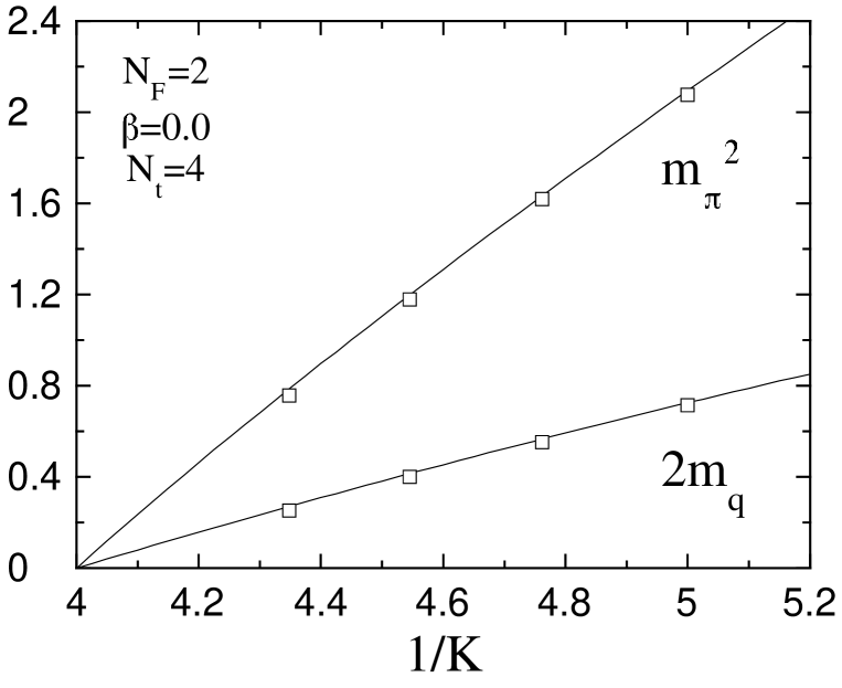
Figure 1: Squared pion screening mass $m_{\pi}^{2}a^{2}$ and twice the quark mass $2m_{q}a$ for $N_{F}=2$ at $\beta=0$ on an $8^{2}\times 10\times 4$ lattice. Errors are smaller than the size of symbols. Solid curves are the results of a strong coupling calculation, Eq.(6).

gives the relation $m_{\pi}^{2}\propto m_{q}$ at small $m_{q}$. Our numerical data for $N_{F}=2$ at $\beta=0$ agrees well with these formulae within errors as shown in Fig. 1.

We note that, if

$$\langle\,0\,|\,A_{4}\,|\,\pi(\vec{p}=0)\,\rangle\propto m_{\pi}$$ (7)

is satisfied for small $m_{q}$ as is the case both for $\beta=0$ and $\beta=\infty$, then the definition (4) implies that the PCAC relation (5) is exact. It should be also noted that Eq.(7) holds when Euclidean invariance is recovered [10].

Eq.(4) implies that when $m_{q}=0$, either $m_{\pi}=0$ or $\langle\,0\,|\,A_{4}\,|\,\pi(\vec{p}=0)\,\rangle=0$. This further implies, when we define the pion decay constant $f_{\pi}$ by

$$\langle\,0\,|\,A_{4}\,|\,\pi(\vec{p}=0)\,\rangle=m_{\pi}f_{\pi},$$ (8)

that when $m_{q}=0$, either $m_{\pi}=0$ or $f_{\pi}=0$ is satisfied. Note that $f_{\pi}=0$ is the relation which should be satisfied when chiral symmetry is restored, and that $m_{\pi}=0$ is the relation when chiral symmetry is spontaneously broken, both in the chiral limit. It might be emphasized that although the action does not possess chiral symmetry, either relation of $m_{\pi}=0$ or $f_{\pi}=0$ holds in the massless quark limit when the quark mass is defined by Eq.(4). In particular, in the confining phase, $m_{\pi}=0$ when $m_{q}=0$ and vice versa.

3.2 Definition of chiral limit and phase structure at zero temperature

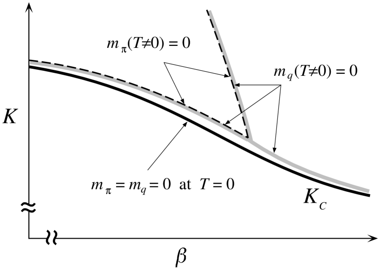
Figure 2: Schematic graph for the chiral limit line $K_{c}$ defined by $m_{q}=0$ or $m_{\pi}=0$ at $T=0$ in the coupling parameter space $(\beta,K)$. Also plotted are the curves where $m_{q}=0$ and $m_{\pi}=0$ at finite $N_{t}$. See text for discussions.

We identify the chiral limit as the limit where the quark mass vanishes at zero temperature. This defines a chiral limit line $K_{c}$ in the $(\beta,K)$ plane, which is a curve from $K\simeq 1/4$ at $\beta=0$ to $K=1/8$ at $\beta=\infty$. See Fig. 2. In the following we also discuss alternative identifications of the chiral limit. When clear specification is required, we denote this $K_{c}$ as $K_{c}(m_{q})$.

Let us denote a line where the pion mass vanishes at zero temperature by $K_{c}(m_{\pi}^{2})$. This line is the critical line of the theory because the partition function has singularities there. As discussed in the previous subsection, we expect that $K_{c}(m_{q})$ and $K_{c}(m_{\pi}^{2})$ are identical for small $N_{F}$. It should be, however, noted that the $K_{c}(m_{q})$ line is conceptually different from the $K_{c}(m_{\pi}^{2})$ line: If quarks are not confined and chiral symmetry is not spontaneously broken, there is no $K_{c}(m_{\pi}^{2})$ line. In fact, for the case of $N_{F}\geq 7$, the $K_{c}(m_{q})$ line belongs to the deconfining phase and $m_{\pi}$ remains nonzero there — i.e. there is no $K_{c}(m_{\pi}^{2})$ line around the $K_{c}(m_{q})$ line, at least for small $\beta$ [12].

As a statistical system on the lattice, QCD with Wilson quarks is well-defined also in the region above the $K_{c}$ line. Some time ago, S. Aoki [17] proposed and numerically verified that the critical line $K_{c}(m_{\pi}^{2})$ (for small $N_{F}$) can be interpreted as a second order phase transition line between the parity conserving phase and a parity violating phase. This interpretation is useful in understanding the existence of singularities of the partition function. Once its existence is established, various properties of hadrons can be investigated in the parity conserving phase. In particular, even with the Wilson term, various amplitudes near the chiral limit do satisfy Ward-Takahashi identities derived from chiral symmetry to the corrections of $O(a)$ [9]. Therefore, although the action does not have chiral symmetry, the concept of the spontaneous breakdown of chiral symmetry is phenomenologically very useful. Because our main interest is to study the physical properties of hadrons in the continuum limit, it is important to study these axial Ward-Takahashi identities and estimate the magnitude of the $O(a)$ corrections from the Wilson term in the physical quantities.

We have defined the $K_{c}$ line by the vanishing point of $m_{q}$ at zero temperature, because this line corresponds to massless QCD. In this connection, however, it should be noted that there necessarily are ambiguities of $O(a)$ off the continuum limit for lines in the $(\beta,K)$ plane which give the same theory in the continuum limit. This is true also for massless QCD: Instead of the condition $m_{\pi}=0$, we may fix other quantities such as $m_{\rho}/m_{N}$, which will lead to a line different from the $K_{c}$ line. Of course, the continuum limit is not affected by these $O(a)$ ambiguities. We, however, would like to stress that the definition we have taken for the $K_{c}$ is conceptually natural and useful for the reasons given in Sec. 3.1.

3.3 Phase structure at finite temperatures

The temperature on a lattice with the linear extension in the temporal direction $N_{t}$ is given by $T=1/{N_{t}a}$. On a lattice with a fixed $N_{t}$, finite temperature transition or crossover from the low temperature regime to the high temperature regime occurs at some hopping parameter when $\beta$ is fixed. This defines a curve $K_{t}$ in the $(\beta,K)$ plane. In this paper, for simplicity, we use the term “transition” for both genuine phase transitions and sharp crossovers, unless explicitly specified. At finite temperatures we denote the screening pion mass by $m_{\pi}$ and sometimes we call it simply the pion mass, and similarly for other hadron screening masses. Quark mass at finite temperatures is defined through Eq.(4) with $m_{\pi}$ the screening pion mass, and similarly for $f_{\pi}$ through Eq.(8). Note that, with these definitions of $m_{\pi}$ and $f_{\pi}$, the discussions given in Sec. 3.1 hold also at finite temperatures.

One of fundamental problems is whether the finite temperature transition line $K_{t}$ does cross the chiral limit line $K_{c}$, where we define the $K_{c}$ line by the vanishing point of $m_{q}$ at zero temperature (cf. Sec. 3.2). If the $K_{t}$ line does not cross the $K_{c}$ line, it means that there is no chiral limit in the low temperature confining phase. Therefore it is natural to expect that it does cross. However, as first noted by Fukugita et al. [18], it is not easy to confirm this: The $K_{t}$ line creeps deep into the strong coupling region. In this paper we show that the $K_{t}$ line indeed crosses the chiral line $K_{c}$ at $\beta\sim 3.9$ — 4.0 at $N_{t}=4$ and $\beta\sim 4.0$ — 4.2 at $N_{t}=6$ for the case of $N_{F}=2$. (For previous reports see Refs.[3, 4].)

Because the $K_{c}$ line describes the massless QCD, we identify the crossing point of the $K_{c}$ and $K_{t}$ lines as the point of the finite temperature transition of the massless QCD, i.e. the chiral transition point. (We will discuss later $O(a)$ ambiguities in the definition of the chiral limit at finite temperatures which come from the lack of chiral symmetry.)

Numerical studies show that, in the confining phase, the pion mass vanishes, for a fixed $\beta$, at the hopping parameter which approximately equals the chiral limit $K_{c}$. On the other hand, in the deconfining phase, the pion mass is of order of twice the lowest Matsubara frequency $2\pi/N_{t}$ in the chiral limit. Therefore, in the deconfining phase, the system is not singular even on the $K_{c}$ line.

Recently, Aoki et al. [19] investigated a critical line where the screening pion mass vanishes at finite temperatures, which we denote by $K_{c}(m_{\pi}^{2};T\neq 0)$. Based on analytic studies of the 2d Gross-Neveu model and numerical results in lattice QCD with $N_{F}=2$, they showed that the $K_{c}(m_{\pi}^{2};T\neq 0)$ line starting from $K\simeq 1/4$ at $\beta=0$ sharply turns back upwards (to larger $K$ region) at finite $\beta$. The lower part of the $K_{c}(m_{\pi}^{2};T\neq 0)$ line is almost identical with the $K_{c}(m_{\pi}^{2})$ line up to the sharp turning point, while the analytic results of the 2d Gross-Neveu model suggest that they slightly differ from each other, probably with $O(a)$. See Fig. 2.

The non-existence of the $K_{c}(m_{\pi}^{2};T\neq 0)$ line in the large $\beta$ region is consistent with the previous results that $m_{\pi}$ does not vanish in the deconfining phase along the chiral line $K_{c}$. The slight shift of the $K_{c}(m_{\pi}^{2};T\neq 0)$ line from the $K_{c}(m_{\pi}^{2})$ line in the confining phase was observed also in our previous study [3, 4] (see also Sec. 5). This slight shift of the $K_{c}(m_{\pi}^{2};T\neq 0)$ line means that $m_{\pi}$ is not rigorously zero on the $K_{c}(m_{\pi}^{2})$ line in the confining phase at finite temperatures. This small pion mass on the $K_{c}$ line in the confining phase is caused by the chiral symmetry violation due to the Wilson term and should be of $O(a)$.

Similarly to the $K_{c}(m_{\pi}^{2};T\neq 0)$ line, we define the line $K_{c}(m_{q};T\neq 0)$ where the quark mass vanishes at finite temperatures. When we follow the line $K_{c}(m_{q};T\neq 0)$ from $\beta=0$, it is first identical with the $K_{c}(m_{\pi}^{2};T\neq 0)$ line. The line $K_{c}(m_{q};T\neq 0)$ passes through the turning point of the $K_{c}(m_{\pi}^{2};T\neq 0)$ line and runs into the larger $\beta$ region, where $f_{\pi}$ starts to vanish instead of $m_{\pi}$ on the $K_{c}(m_{q};T\neq 0)$ line. See Fig. 2. This suggests that the turning point which is the boundary between $f_{\pi}=0$ and $m_{\pi}=0$ is the finite temperature transition point. This further implies that the transition line $K_{t}$ touches the turning point of the $K_{c}(m_{\pi}^{2};T\neq 0)$ line and moves upwards in the $(\beta,K)$ plane. This observation is not in accord with the argument by Aoki et al. [19] that there is a small gap between the $K_{c}(m_{\pi}^{2};T\neq 0)$ and $K_{t}$ lines.

We have identified the crossing point of the $K_{c}$ and $K_{t}$ lines as the chiral transition point. In connection with the $O(a)$ ambiguities of the line for massless QCD in the coupling parameter space mentioned in Sec. 3.2, there are $O(a)$ ambiguities also in the definition of the chiral transition. Therefore, one may alternatively identify the sharp turning point of the $K_{c}(m_{\pi}^{2};T\neq 0)$ line as the chiral transition point. The property of the chiral transition in the continuum limit is, of course, not affected by these $O(a)$ ambiguities.

3.4 Characteristics for Wilson quarks

Let us summarize several characteristic properties of the phase diagram of QCD which are originated from the explicit chiral symmetry violation of the Wilson term. They are in sharp contrast with those of staggered quarks where at least a part of chiral symmetry is preserved.

(i) In the coupling parameter space, the location of the point where $m_{\pi}=0$ in the confining phase is not protected by chiral symmetry off the continuum limit. Therefore, the chiral limit $K_{c}$, defined by $m_{q}=0$ or $m_{\pi}=0$ at zero temperature, is different from the bare massless limit $K=1/8$ except at $\beta=\infty$.

(ii) As a statistical system on the lattice, QCD with Wilson quarks is well-defined also in the region above the $K_{c}$ line. At zero temperature, the $K_{c}$ line is a second order transition line between the conventional parity conserving phase at $K<K_{c}$ and a parity violating phase at $K>K_{c}$ [17].

(iii) At finite temperatures, the critical line $K_{c}(m_{\pi}^{2};T\neq 0)$ where the screening pion mass vanishes is not a line from $K\simeq 1/4$ at $\beta=0$ to an end at some finite $\beta$, but it sharply turns back toward larger $K$ region at the finite $\beta$ [19].

(iv) Although the major part of the effects from the Wilson term can be absorbed by the shift of $K_{c}$ from $K=1/8$, there still exist additional small $O(a)$ effects which are related to the chiral symmetry violation. In particular, the location of the point where $m_{\pi}=0$ in the confining phase slightly depends on $N_{t}$ [19]. The continuum limit is not affected by these $O(a)$ effects.

4 Simulation Parameters

In this article we mainly perform simulations on lattices with the temporal direction extension $N_{t}=4$. The spatial sizes are $8^{2}\times 10$ and $12^{3}$. To study the $N_{t}$ dependence for the $N_{F}=2$ case, we also make simulations on $N_{t}=6$ and 8 lattices. Simulations on an $N_{t}=8$ lattice are performed also for the case of $N_{F}=2+1$. When the hadron spectrum is calculated, the lattice is duplicated in a direction of lattice size 10 or 12. We use an anti-periodic boundary condition for quarks in the $t$ direction and periodic boundary conditions otherwise.

We generate gauge configurations for $N_{F}=2$ by the Hybrid Monte Calro (HMC) algorithm [20] with a molecular dynamics time step $\Delta\tau$ chosen in such a way that the acceptance rate is about 80 — 90%. For $N_{F}\geq 3$ and $N_{F}=2+1$ we use the hybrid R algorithm [21] with $\Delta\tau=0.01$, unless otherwise stated. We fix the time length of each molecular dynamics evolution to $\tau=1$. The R algorithm introduces errors of $O(\Delta\tau^{2})$, while the HMC algorithm is exact. As reported recently also for staggered quarks [22], we note that step size errors with the R algorithm are large in the confining phase near the chiral limit. In the immediate vicinity of the chiral transition, we observe step size errors also in the deconfining phase where a large $\Delta\tau$ can even push the phase into the confining phase, as reported previously with staggered quarks [23]. In these cases, we apply a sufficiently small $\Delta\tau$ so that the results for physical quantities become stable for a change of $\Delta\tau$.

The inversion of the quark matrix is done by the minimal conjugate residual (CR) method with the ILU preconditioning [24] or the conjugate gradient (CG) method without preconditioning. We find that the CR method is efficient in the confining phase when it is not very close to the chiral limit and also in the deconfining phase at large $\beta$ and small $K$. In other cases we use the CG method. The convergence condition for the norm of the residual $r$ is $\sqrt{\|r\|^{2}/(12V)}\leq 4.5\times 10^{-7}$ ($1.0\times 10^{-8}$) for configuration generations (hadron measurements), where $V$ is the lattice volume. We also check that the relative changes of the quark propagator at several test points on the $x$ and $t$ axes are smaller than $10^{-3}$ for the last iteration of the matrix inversion steps: $|(G_{n}-G_{n-1})/G_{n}|\leq 10^{-3}$ where $n$ denotes the last iteration. In the HMC calculations, we check that the difference of the action after molecular dynamic evolutions is sufficiently small with this convergence condition.

The statistics is in general totally $\tau=$ several hundreds. The initial configuration is taken from a thermalized one at similar simulation parameters when such a configuration is available. In most cases, the plaquette and the Polyakov loop are measured every simulation time unit and hadron spectrum is calculated every $\delta\tau=10$ (or less depending on the total statistics). When the value of $\beta$ is small the fluctuation of physical quantities are small [12], and therefore we think the lattice sizes and the statistics are sufficient for our purpose to determine the global phase structure of QCD at finite temperature. Errors are estimated by the single-elimination jackknife method.

Simulation parameters are summarized in Tables 1 — 9.

5 Numerical results for $K_{c}$

As discussed in Sec. 3.2, the chiral limit $K_{c}$ is defined by the vanishing point of $m_{q}$ at zero temperature. One straightforward way to determine numerically the chiral limit at a fixed value of $\beta$ is to calculate the the quark mass through Eq.(4) at several hopping parameters and extrapolate them to its vanishing point in terms of a linear function of $1/K$. We denote the $K_{c}$ thus determined by $K_{c}(m_{q})$. Because we expect the PCAC relation (5) to hold also at finite $\beta$, we may alternatively calculate $K_{c}$ by the vanishing point of $m_{\pi}$ using a linear extrapolation of $m_{\pi}^{2}$ in $1/K$. We denote this $K_{c}$ by $K_{c}(m_{\pi}^{2})$.

On finite temperature lattices, it was previously shown that the value of the quark mass at given $(\beta,K)$ does not depend on whether the system is in the deconfining or confining phase at $\beta=5.85$ in the quenched QCD [14] and at $\beta=5.5$ for the $N_{F}=2$ case [13]. This enables us to determine the chiral limit, for these values of $\beta$, alternatively by the vanishing point of $m_{q}$ at finite temperatures. Strictly speaking there are systematic errors which come from finite $N_{t}$, as mentioned earlier. On the other hand, in the deconfining phase, one is able to perform simulations around the $K_{c}$ line as discussed later, i.e. we can determine $K_{c}$ without an extrapolation which usually leads to a considerable amount of systematic errors. Therefore, the determination of $K_{c}$ from $m_{q}$ in the deconfining phase is useful in particular at large $\beta$.

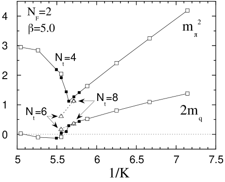
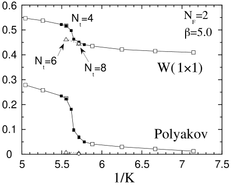
Figure 3: Physical quantities for $N_{F}=2$ at $\beta=5.0$ on an $8^{2}\times 10\times 4$ lattice (open squares): (a) $m_{\pi}^{2}a^{2}$ and $2m_{q}a$, (b) the plaquette and the Polyakov loop. Plotted together are the data by the MILC collaboration on an $8^{2}\times 20\times N_{t}$ lattice with $N_{t}=4$ (filled squares), 6 (triangles), and 8 (diamonds) [16]. The finite temperature transition $K_{t}$ obtained by the MILC data locates at $K=0.177$ — 0.178 ($1/K=5.62$ — 5.65) for $N_{t}=4$.

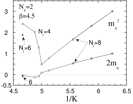
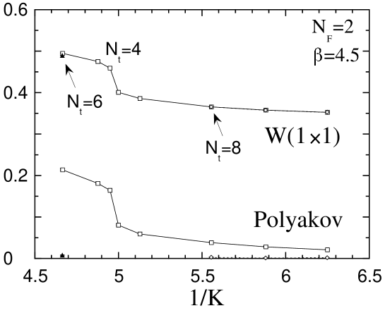
Figure 4: The same as Fig. 3 at $\beta=4.5$ on $8^{2}\times 10\times N_{t}$ lattices, where $N_{t}=4$ (squares), 6 (triangles), and 8 (diamonds). The finite temperature transition $K_{t}$ locates at $K=0.200$ — 0.202 ($1/K=4.95$ — 5.0) for $N_{t}=4$.

At small $\beta$ region ($\beta$ $<$$\sim$ 5.3) where we mainly perform simulations in this work, $m_{q}$ in the deconfining phase does not agree with that in the confining phase. Therefore, the proportionality between $m_{q}$ in the deconfining phase and $m_{\pi}^{2}$ in the confining phase is lost, contrary to the case $\beta$ $>$$\sim$ 5.5 discussed above. This behavior is seen in Figs. 3 and 4, where physical quantities for $N_{F}=2$ at $\beta=5.0$ and 4.5, respectively, are shown. As we discuss in Sec. 6, we interpret this unexpected phenomenon at $\beta$ $<$$\sim$ 5.3 in the deconfining phase as a lattice artifact.

In the confining phase, on the other hand, the proportionality between $m_{q}$ and $m_{\pi}^{2}$ is well satisfied for all values of $\beta$ [3, 12, 13, 14, 15, 16]. We also find that $m_{q}$ and $m_{\pi}$ are almost independent of $N_{t}$ in the confining phase. See Fig. 4 for $N_{F}=2$ at $\beta=4.5$. Therefore we can calculate $K_{c}$ approximately also by the vanishing point of $m_{q}$, $K_{c}(m_{q})$, or that of $m_{\pi}^{2}$, $K_{c}(m_{\pi}^{2})$, in the confining phase at $T>0$.

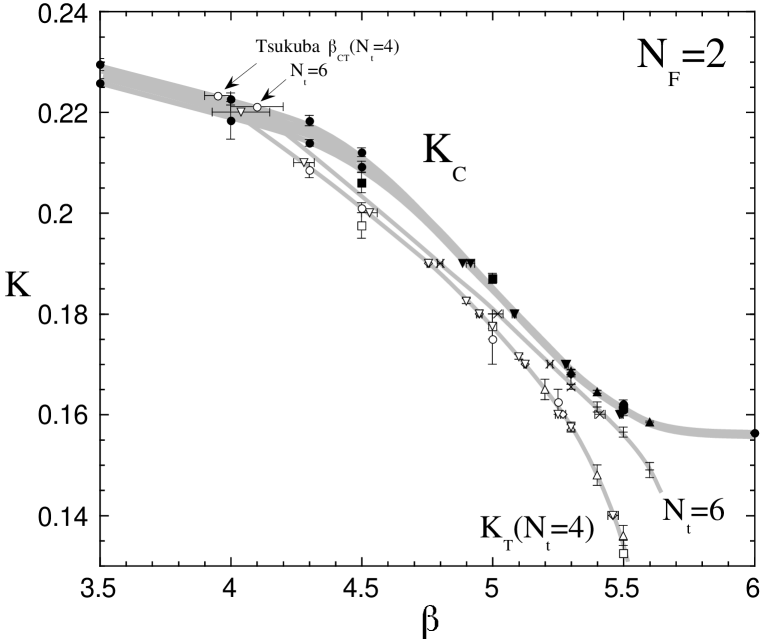
Figure 5: Phase diagram for $N_{F}=2$. Filled symbols are for $K_{c}$ determined by $m_{\pi}=0$ and $m_{q}=0$. Open symbols are for $K_{t}(N_{t}=4)$ and other symbols such as crosses except filled ones are for $K_{t}(N_{t}=6)$. Circles are our data. Lines are to guide the eyes.

The numerical results for $K_{c}$ for $N_{F}=2$ obtained by various groups [3, 13, 25, 26, 27, 28, 29] are plotted in Fig. 5 together with finite temperature transition lines discussed in the following sections. The values of $K_{c}$ show a slight dependence (at most of the order of 0.01) on the choice of $K_{c}(m_{q})$ or $K_{c}(m_{\pi}^{2})$, which can be probably attributed to the systematic errors in the extrapolation of $m_{\pi}^{2}$ and $m_{q}$ in $1/K$, because, as discussed above, we expect that $K_{c}(m_{q})$ and $K_{c}(m_{\pi}^{2})$ are identical. The values of $K_{c}(m_{\pi}^{2})$ for $N_{F}=2$ for various $\beta$’s are listed in Table 10. We estimate the systematic errors due to the extrapolation are of the same order as the differences between $K_{c}(m_{q})$ and $K_{c}(m_{\pi}^{2})$.

The $N_{t}$ dependence of $K_{c}$ at $\beta=4.5$ are listed in Table 11. The $N_{F}$ dependence is also given. We find that the differences due to $N_{F}$ and $N_{t}$ are of the same order of magnitude as the difference between $K_{c}(m_{q})$ and $K_{c}(m_{\pi}^{2})$.

To summarize this section, we note that although the chiral limit is defined by the vanishing point of $m_{q}$ at zero temperature, there are several practically useful ways to determine $K_{c}$: $K_{c}(m_{q})$ and $K_{c}(m_{\pi}^{2})$ at $T=0$ and in the confining phase, and $K_{c}(m_{q})$ in the deconfining phase. They all gives the same results within present numerical errors.

6 Finite Temperature Transition and Problems with Wilson Quarks

The location of the finite temperature phase transition $K_{t}$ is identified by a sudden change of physical observables such as the plaquette, the Polyakov line and screening hadron masses. (A more precise determination of the location will be given by the maximum point of the susceptibility of a physical quantity such as the Polyakov loop. However, our statistics is not high enough for it.) See Figs. 3 and 4 for the case of $N_{F}=2$ at $\beta=5.0$ and 4.5. Our numerical results of $K_{t}$ are summarized in Table 12. Results of $K_{t}$ for $N_{F}=2$ at $N_{t}=4$ and 6 obtained by us and other groups [16, 26, 29, 30, 31] are compiled in Fig. 5. (Results for $N_{F}=3$ will be discussed in Sec. 8.)

We expect, at least near the continuum limit, that as the quark mass increases from the chiral limit, the transition becomes weaker with the quark mass and it becomes strong again when the quark mass is heavy enough to recover the first order transition of the SU(3) gauge theory. The MILC collaboration performed a systematic study of the transition at various $K$ and $\beta$ and found that, contrary to the expectation, when we decrease $K$ from the chiral limit $K_{c}$ on an $N_{t}=4$ lattice, the $K_{t}$ transition becomes once very strong at $K\simeq 0.18$ and becomes weaker again at smaller $K$ [16]. On a lattice with $N_{t}=6$ they even found a first order transition at $K=0.17$ — 0.19 [29].

Looking at the phase diagram shown in Fig. 5 closely, we note that the $K_{t}$ lines initially deviate from the $K_{c}$ line and then approach the $K_{c}$ line at $\beta\sim 4.8$ and $K\sim 0.18$ for $N_{t}=4$ and at $\beta\sim 4.8$ — 5.2 and $K\sim 0.17$ — 0.19 for $N_{t}=6$, contrary to the naive expectation that they monotonously deviate from the $K_{c}$ line. The points where strong transitions occur are just in the region where the $K_{t}$ lines approach the $K_{c}$ line. Therefore, it is plausible that the strong transition at intermediate values of $K$ is a result of lattice artifacts caused by this unusual relation of the $K_{t}$ and $K_{c}$ lines [7]. This unusual relation is probably due to the sharp bend of the $K_{c}$ line at $\beta\simeq 5.0$ which is caused by the cross-over phenomenon between weak and strong coupling regions of QCD. Our recent study indeed shows that, with an improved lattice action, the distance between the the $K_{c}$ and $K_{t}$ lines becomes monotonically large when we decrease $K$ and, correspondingly, the $K_{t}$ transition becomes rapidly weak as we decrease $K$ from the chiral limit [32]. Also the unexpected $N_{t}$ dependence of $m_{q}$ in the deconfining phase at small $\beta$ discussed in the previous section, is removed with the same improved lattice action.

The appearance of the lattice artifacts implies that we have to be cautious when we try to derive the conclusions in the continuum limit from the numerical results at finite $\beta$. We also note that $N_{t}=4$ is far from the continuum limit and therefore we should take with reservation, in particular, quantitative values in physical units which are quoted in the following. We, however, note that the PCAC relation $m_{\pi}^{2}\propto m_{q}$ expected from chiral symmetry in the confining phase is well satisfied even in the strong coupling region and therefore we expect that qualitative feature of the chiral transition such as the order of the transition does not affected by lattice artifacts. We certainly have to check in future that the conclusions in this article are also satisfied when an improved action is adopted.

7 Numerical Results for Chiral Transitions

As discussed in Sec. 3.3, the chiral transition can be studied along the $K_{c}$ line at the crossing point of the $K_{t}$ and $K_{c}$ lines, which we denote as the chiral transition point $\beta_{ct}$. We first address ourselves to the problem of whether the chiral limit of the finite temperature transition exists at all. We then study the order of the chiral transition.

In a previous paper [12] we showed that, when $N_{F}\geq 7$, there is a bulk first order phase transition at $\beta=0$ which separates the confining phase at small $K$ from a deconfining phase near the chiral limit at $K=1/4$. This implies that the $K_{t}$ line does not cross the $K_{c}$ line at finite $\beta$ for any $N_{t}$. On the other hand, when $N_{F}\leq 6$, the chiral limit belongs to the confining phase at $\beta=0$, which implies that there is a crossing point somewhere at finite $\beta$ for the case $N_{F}\leq 6$.

7.1 On-$K_{c}$ method

In order to identify the crossing point $\beta_{ct}$ and study the order of the chiral transition there, we take the strategy of performing simulations on the $K_{c}$ line starting from a value of $\beta$ in the deconfining phase and reducing $\beta$. We call this method “on-$K_{c}$” simulation method. The number of iterations $N_{\rm inv}$ needed for the quark matrix inversion, in general, provides a good indicator to discriminate the deconfining phase from the confining phase [14, 33]. The use of $N_{\rm inv}$ as an indicator is extremely useful on the $K_{c}$ line, because $N_{\rm inv}$ is enormously large on the $K_{c}$ line in the confining phase, while it is of order several hundreds in the deconfining phase. Therefore there is a sudden drastic change of $N_{\rm inv}$ across the boundary of the two phases. This difference is due to the fact that there are zero modes around $K_{c}$ in the confining phase, while none exists in the deconfining phase [12, 33, 34]: We have checked this difference for the existence of zero modes in various cases discussed below and conclude that the difference of $N_{\rm inv}$ is not a numerical artifact.

In the deconfining phase on the $K_{c}$ line, we measure physical observables such as the Polyakov loop, the plaquette and hadron screening masses, as usual, after thermalization. From the behavior of physical quantities toward $\beta_{ct}$, we are able to study the nature of the chiral transition. In the confining phase, on the other hand, it is hard to make the system on the $K_{c}$ line thermalized due to the enormously large $N_{\rm inv}$ we encounter in the configuration generation. In this case, we only obtain at most bounds for several physical quantities by measuring the molecular dynamic time evolution of them starting a hot state or a mix state. Although it is unsatisfactory that we cannot obtain expectation values for physical quantities in the confining phase, the on-$K_{c}$ method is very powerful to identify the critical point because the difference between the two phases is clear already with short time-histories. We also check that the crossing point thus determined is consistent with a linear extrapolation of the line $K_{t}$ toward the chiral limit.

7.2 Chiral transition for $N_{F}=2$

For the case of QCD with two flavors, studies of an effective $\sigma$ model[1, 2] imply that the order of the chiral transition depends on the the strength of the U$\!{}_{A}$(1) anomaly term at the transition temperature. When the strength is zero, it is of first order. However, if the strength of the anomaly term in the effective $\sigma$ model is non-zero at the starting point of renormalization transformation, it is likely that the effective action is attracted to a $O(4)$ symmetric fixed point under renormalization group transformation [35]. Therefore, it is plausible that the chiral transition is of second order.

Our main results of the measurements for $N_{F}=2$ are summarized in Tables 13 — 15.

Let us first discuss the results at $N_{t}=4$. In order to confirm the existence of the crossing point, we take the largest (farthest) values of $K_{c}$ for on-$K_{c}$ simulations, that is, $K_{c}(m_{\pi}^{2})$ for $N_{F}=2$ in Table 10 and interpolated ones. As discussed previously, $K_{c}(m_{\pi}^{2})$ in general depend on the value of $N_{t}$. However, the differences between those on the $N_{t}=4$ and 8 lattices are within numerical uncertainties as shown Table 11. Therefore, we take the stringent condition to verify the existence of the crossing point, taking the farthest values of $K_{c}$.

When we take into account the structure of $K_{c}(m_{\pi}^{2};T\neq 0)$ that it sharply turns back at finite $\beta$, we may hit the upper part of it by taking the largest values of $K_{c}$ for the “on-$K_{c}$” method. This, however, does not affect the conclusion that the $K_{t}$ line crosses the $K_{c}$ line. Our estimates for the value of $\beta_{ct}$ in this case will be slightly underestimated (cf. Fig. 2). This comment applies also for $N_{F}=3$ and 6.

We first perform on-$K_{c}$ simulations by the R algorithm to identify the crossing point, because it is very time consuming to perform simulations with the HMC algorithm due to a low acceptance rate on the $K_{c}$ line in the confining phase. We find that when $\beta\geq 4.0$, $N_{\rm inv}$ stays around several hundreds, while for $\beta\leq 3.9$ it increases with $\tau$ and exceeds several thousands (see Fig. 6) and in accord with this behavior the plaquette, the Polyakov loop and $m_{\pi}$ decrease rapidly toward those in the confining phase. Therefore we identify the crossing point at $\beta_{ct}\sim 3.9$ — 4.0. This $\beta_{ct}$ is consistent with a linear extrapolation of the $K_{t}$ line as is shown in Fig. 5.

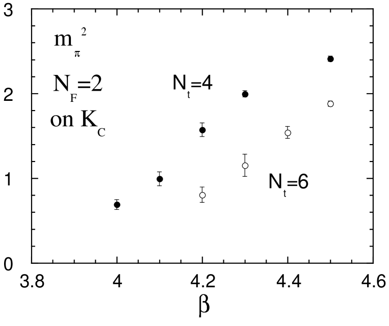
Figure 7: The pion screening mass squared $m_{\pi}^{2}a^{2}$ for $N_{F}=2$ on the $K_{c}$ line obtained on $8^{2}\times 10\times 4$ and $12^{3}\times 6$ lattices.

Then we repeat on-$K_{c}$ simulations by the HMC algorithm for $\beta\geq 4.0$ in order to measure physical observables. The time histories for $N_{\rm inv}$ at $\beta\geq 4.0$ plotted in Fig. 6 are obtained with the HMC algorithm, which are similar to those with the R algorithm. The $\Delta\tau$ should be taken small near $\beta_{ct}$ in order to keep the acceptance rate reasonably high (for $\beta=4.0$, 4.1 and 4.2 we use $\Delta\tau=0.002$, 0.005 and 0.005 to get acceptance rates 0.91, 0.79 and 0.93, respectively). The value of $m_{\pi}^{2}$ thus obtained decreases smoothly toward zero as the chiral transition is approached and is consistent with zero at the estimated $\beta_{ct}$ (see Fig. 7).

We find no two-state signals around $\beta_{ct}$. This is in sharp contrast with the $N_{F}=3$ and 6 cases where we find clear two-state signals at $\beta_{ct}$, as discussed below. This, together with the vanishing $m_{\pi}^{2}$ toward $\beta_{ct}$, indicates that the chiral transition is continuous (second order or crossover) for $N_{F}=2$.

The results from on-$K_{c}$ simulations on the $N_{t}=6$ lattice are similar to those on the $N_{t}=4$ lattice. The estimated transition point is $\beta_{ct}\sim$ 4.0 — 4.2. The value of $m_{\pi}^{2}$ listed in Table 14 and plotted in Fig. 7, again decreases toward zero as $\beta$ approaches $\beta_{ct}$. For $N_{t}=18$ with the spatial size $18^{2}\times 24$, we previously found that the transition is at $\beta_{ct}\sim 4.5$ — 5.0 [3]. Although the spatial size is not large enough, this result suggests that the shift of $\beta_{ct}$ with $N_{t}$ is very slow.

7.3 Chiral transition for $N_{F}=3$

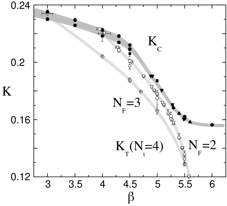
Figure 8: Phase diagram for $N_{F}=2$ and 3. Filled symbols are for $K_{c}(m_{\pi}^{2})$ and $K_{c}(m_{q})$. Open symbols are for $K_{t}(N_{t}=4)$ for $N_{F}=2$ and open circles with cross for $N_{F}=3$. Circles are our data. On the $K_{t}$ line for $N_{F}=3$, clear two-state signals are observed at $\beta\leq 4.7$ both on $8^{2}\times 10\times 4$ and $12^{3}\times 4$ lattices. Lines are to guide the eyes.

Main results of measurements for $N_{F}=3$ are summarized in Tables 16 and 17. The phase diagram for $N_{F}=3$ obtained from our simulations at $\beta$=4.0, 4.5, 4.7, 5.0 and 5.5 is shown in Fig. 8. We find that the $K_{t}$ line linearly approaches to the $K_{c}$ line. In order to confirm the existence of the crossing point by on-$K_{c}$ simulations, we take the largest (farthest) $K_{c}$, that is $K_{c}(m_{\pi}^{2})$ for $N_{F}=2$ at $\beta$’s we have studied, since this is the most stringent condition for the existence of $\beta_{ct}$. We use them and interpolated values for on-$K_{c}$ simulations here. For $N_{F}=6$ discussed in the next subsection, we interpolate these values of $K_{c}$ with $K_{c}=0.25$ at $\beta=0$. Note that the differences of $K_{c}$’s for $N_{F}=2$, 3 and 6 are of the same magnitude of numerical uncertainties of $K_{c}$.

Fig. 9 shows $N_{\rm inv}$ as a function of the molecular-dynamics time $\tau$ for several values of $\beta$’s. When $\beta\geq 3.1$, $N_{\rm inv}$ is of order of several hundreds, while when $\beta\leq 2.9$, $N_{\rm inv}$ shows a rapid increase with $\tau$. At $\beta=3.0$ we see a clear two-state signal depending on the initial condition: For a hot start, $N_{\rm inv}$ is quite stable around $\sim 800$ and $m_{\pi}^{2}$ is large ($\sim 1.0$). On the other hand, for a mix start, $N_{\rm inv}$ shows a rapid increase with $\tau$ and exceeds 2,000 in $\tau\sim 20$, and in accordance with this, $m_{\pi}^{2}$ decreases with $\tau$.

The value of $m_{\pi}^{2}$ is plotted in Fig. 10. At $\beta=3.0$ we have two values for $m_{\pi}^{2}$ depending on the initial configuration. The larger one obtained for the hot start is of order 1.0, which is a smooth extrapolation of the values at $\beta\sim 3.1$ - 3.2. The smaller one is an upper bound for $m_{\pi}^{2}$ for the mix start.

We note that the result of $\beta_{ct}\sim 3.0$ is consistent with an extrapolation of $K_{t}$ points listed in Table 12 as is shown in Fig. 8. (The nature of the transition $K_{t}$ off the chiral limit is discussed in Sec. 8.) Thus we identify the crossing point at $\beta_{ct}\sim 3.0(1)$. With the clear two-state signal we conclude that the chiral transition is of first order for $N_{F}=3$.

7.4 Chiral transition for $N_{F}$ = 6

Our previous study at $\beta=0$ [12] shows that for $N_{F}=7$ there is no crossing point of the $K_{c}$ and $K_{t}$ lines and that $N_{F}=6$ is the largest number of flavors for which a crossing point exists. Main results of measurements for $N_{F}=6$ are summarized in Table 18. Overall features of the transition obtained from numerical simulations for $N_{F}=6$ are very similar to those for $N_{F}=3$ except for the location of $\beta_{ct}$, which moves to a smaller $\beta$ as expected. Fig. 11 shows that $N_{\rm inv}$ on the $K_{c}$ line stays at several hundreds for $\beta\geq 0.4$ and for a hot start at $\beta=0.3$. On the other hand, $N_{\rm inv}$ grows rapidly with $\tau$ and exceeds 5,000 for $\beta\leq 0.2$ and for a mix start at $\beta=0.3$. In accord with this, we have two values of $m_{\pi}^{2}$ at $\beta=0.3$ (cf. Fig. 12). Therefore we identify the crossing point at $\beta_{ct}\sim 0.3(1)$ and conclude that the chiral transition is of first order for $N_{F}=6$. This $\beta_{ct}$ is consistent with a linear extrapolation of the $K_{t}$ line (cf. Table 12).

For QCD with $N_{F}\geq 3$, Pisarski and Wilczek predicted a first order chiral transition from a renormalization group study of an effective $\sigma$ model [1]. Our results for $N_{F}=3$ and 6 are consistent with their prediction.

8 Influence of the Strange Quark

In the previous section, we have seen that the chiral transition is consistent with a second order transition for $N_{F}=2$, while it is of first order for $N_{F}\geq 3$, both in accordance with theoretical expectations. Off the chiral limit, we expect that the first order transition for $N_{F}\geq 3$ smoothens into a crossover at sufficiently large $m_{q}$. In this way the nature of the transition sensitively depends on $N_{F}$ and $m_{q}$. Therefore, in order to study the nature of the transition in the real world, we should include the strange quark properly whose mass $m_{s}$ is of the same order of magnitude as the transition temperature $T_{c}\simeq 100$ — 200 MeV.

In a numerical study we are able to vary the mass of the strange quark. When the mass of the strange quark is reduced from infinity to zero with up and down quarks fixed to the chiral limit, the nature of the transition must change from continuous to first order at some quark mass $m_{s}^{*}$. Assuming that the chiral transition is of second order for $N_{F}=2$ (i.e. $m_{s}=\infty$), this point at $m_{s}^{*}$ is a tricritical point [2]. The crucial question is whether the physical strange quark mass is larger or smaller than $m_{s}^{*}$. Studies with an effective linear $\sigma$ model suggest a crossover for the case of realistic quark masses in meanfield approximation and in a large $1/N_{F}$ approximation [36, 37], while the possibility of a weakly first order transition is not excluded when numerical errors in the calculation of basic parameters are taken into account [37].

8.1 $N_{F}=3$

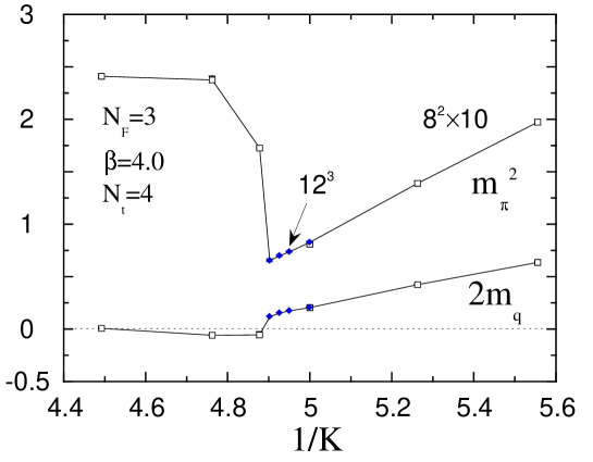
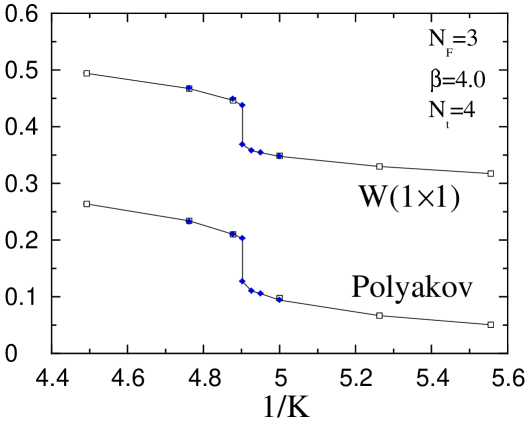
Figure 13: Physical quantities for $N_{F}=3$ at $\beta=4.0$ on $8^{2}\times 10\times 4$ (open squares) and $12^{3}\times 4$ (filled diamonds) lattices: (a) $m_{\pi}^{2}a^{2}$ and $2m_{q}a$, (b) the plaquette and the Polyakov loop. The finite temperature transition $K_{t}$ locates at $K\simeq 0.204$ ($1/K\simeq 4.90$).

Let us first discuss the case of the degenerate $N_{F}=3$: $K_{u}=K_{d}=K_{s}\equiv K$. As we have already discussed the chiral transition previously, we are mainly interested in the transition for the massive quarks. In order to find the transition points we perform simulations at $\beta$=4.0, 4.5, 4.7, 5.0 and 5.5. The results for physical quantities are plotted in Figs. 13 — 17. The transition points identified by a sudden change of physical observables are given in Table 12 and plotted in Fig. 8. We note that the $K_{t}$ line for $N_{F}=3$ at $N_{t}=4$ locates sufficiently far from the points where the $K_{c}$ line bends rapidly. This situation is quite different from the $N_{F}=2$ case where the unusual relation between the $K_{t}$ line and $K_{c}$ line causes the lattice artifacts. Therefore, we expect that these lattice artifacts are small in the $N_{F}=3$ case.

In the previous section we have seen that the transition is of first order in the chiral limit $K_{c}=0.235$ at $\beta=3.0$ for $N_{F}=3$. For phenomenological applications, it is important to estimate the critical value of the quark mass $m_{q}^{crit}$ up to which the first order phase transition persists.

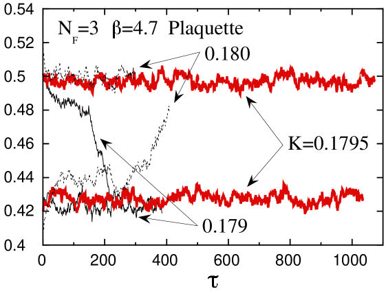
Figure 18: Time history of the plaquette for $N_{F}=3$ at (a) $\beta=4.7$ and (b) 5.0 on a $12^{3}\times 4$ lattice.

We observe clear two state signals at $\beta$ = 4.0, 4.5 and 4.7, while for $\beta=5.0$ and $5.5$ no such signals have been seen: The simulation time history of the plaquette at $\beta=4.7$ on a $12^{3}\times 4$ lattice is plotted in Fig. 18(a). The confining and deconfining phases coexist over 1,000 trajectories at $K=0.1795$ and, in accordance with this, we find two-state signals also in other observables such as the plaquette and the pion screening mass $m_{\pi}$ (cf. Fig. 15). From them we conclude that the transition at $K=0.1795(5)$ and $\beta=4.7$ is first order. On the other hand, the time history of the plaquette at $\beta=5.0$ shown in Fig. 18(b) suggests that the transition is a crossover there.

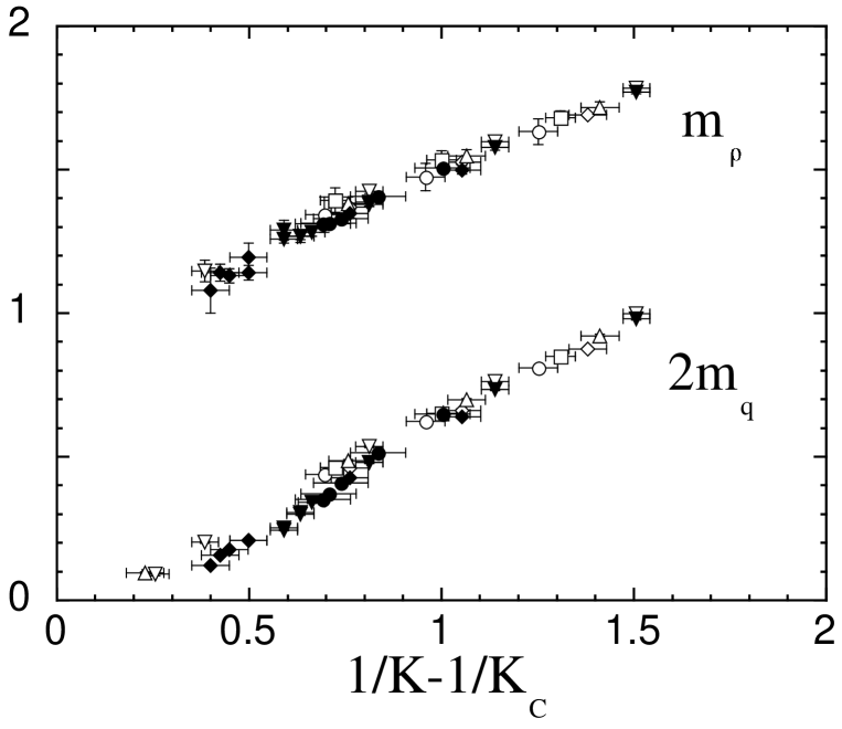
Figure 19: The rho meson screening mass $m_{\rho}a$ and twice the quark mass $2m_{q}a$ in the confining phase as a function of $1/K-1/K_{c}$. Open symbols are for $N_{F}=2$, $\beta=3.0$, 3.5, 4.0, 4.3, and 4.5 on an $8^{2}\times 10\times 4$ lattice. Filled symbols are for $N_{F}=3$, $\beta=4.0$, 4.5 and 4.7 on $8^{2}\times 10\times 4$ and $12^{3}\times 4$ lattices. The values of $K_{c}(\beta)$ for $N_{F}=2$ is used. Horizontal errors are from those for $K_{c}$ with taking into account the difference due to definitions, either the vanishing point of $m_{\pi}^{2}$ or $m_{q}$.

At the transition point (in the confining phase) of $\beta=4.7$ the value of $m_{q}a$ is 0.175(2) and $m_{\pi}/m_{\rho}=0.873(6)$. The results of the hadron spectrum in the range of $\beta=3.0$ – 4.7 for $N_{F}=2$ and 3 (cf. Fig. 19) indicate that the inverse lattice spacing $a^{-1}$ estimated from the rho meson mass is almost independent on $\beta$ in this range and $a^{-1}\sim 0.8$ GeV. (Hereafter we use $a^{-1}$ determined from $m_{\rho}$ in the chiral limit.) Therefore we obtain a bound on the critical quark mass $m_{q}^{crit}\mathop{\vtop{\halign{#\cr$\hfil\displaystyle{>}\hfil$\crcr\kern 0.5pt\nointerlineskip\cr$\sim$\crcr\kern 0.5pt\cr}}}\limits 140$ MeV, or equivalently $(m_{\pi}/m_{\rho})^{crit}\geq 0.873(6)$. It should be noted that the physical strange quark mass determined from $m_{\phi}=1020$ MeV, using the data shown in Fig. 19, turns out to be $m_{s}\sim 150$ MeV in this $\beta$ range with our definition of the quark mass.

We note that these values for the critical quark mass are much larger than those with staggered quarks where $m_{q}^{crit}a=0.025$ — 0.075 [38, 39] ($m_{q}^{crit}\sim 10$ — 40 MeV using $a^{-1}\sim 0.5$ GeV at $\beta=5.2$ for $N_{F}=2$ [40]) which means that $(m_{\pi}/m_{\rho})^{crit}\simeq 0.42$ — 0.58 (using the results of meson masses for $N_{F}=4$ at $\beta=5.2$ [41], because the data for $N_{F}=3$ are not available).

8.2 $N_{F}=2+1$

Now let us discuss a more realistic case of massless up and down quarks and a light strange quark ($N_{F}=2+1$). Main results of measurements are summarized in Tables 19 — 21. Our strategy to study the phase structure is similar to that applied in Sec. 7 for the investigation of the chiral transition in the degenerate quark mass cases, which we called the on-$K_{c}$ method. We set the value of masses for the up and down quarks $m_{ud}$ to zero ($K_{ud}=K_{c}$) and fix the strange quark mass $m_{s}$ to some value, and make simulations starting from a value of $\beta$ in the deconfining phase and reducing the value of $\beta$. When u and d quarks are massless, the number of iteration $N_{\rm inv}$ needed for the quark matrix inversion (for u and d quarks) is enormously large in the confining phase, while it is of order of several hundreds in the deconfining phase. The values which we take for $K_{c}$ are given in Table 22. They are the vanishing point of extrapolated $m_{\pi}^{2}$ for $N_{F}=2$ and interpolated ones. We have used those for $N_{F}=2$, because we have the data most in this case, and the difference between that for $N_{F}=2$ and 3 is of the same order of magnitude as the difference due to the definition of $K_{c}$ (cf. discussions in Sec. 7).

We study two cases of $m_{s}\sim 150$ MeV and 400 MeV. From the value of $a^{-1}\sim 0.8$ GeV and an empirical rule $m_{q}a\simeq(2/3)(1/K-1/K_{c})$ satisfied for $N_{F}=2$ and 3 in the $\beta$ region we have studied (cf. Fig. 19), we get the values for $K_{s}$ shown in Table 22.

In order to confirm that our choice of parameters for the case $m_{s}\sim 150$ MeV is really close to the physical values, we have also made a zero-temperature spectroscopy calculation for the $N_{F}=2+1$ case at $\beta=3.5$ on an $8^{3}\times 10$ lattice. Keeping $K_{s}=0.2017$ ($m_{s}\sim 150$ MeV), we vary $K_{ud}$ from 0.195 to 0.210 in steps of 0.005. Taking the chiral limit of $K_{ud}$, we obtain $a^{-1}=903(38)$ MeV from the rho meson mass ($m_{\rho}a=0.853(36)$ at $K_{c}=0.2227$, where $K_{c}$ is determined by a linear extrapolation of $m_{\pi}^{2}a^{2}$ in terms of $1/K$). The mass of the $\phi$ meson at the simulation point turns out to be 1.03(5) GeV which should be compared with the physical value 1.02 GeV. Thus the hopping parameter chosen for $m_{s}\sim 150$ MeV corresponds to the physical strange quark mass, in this sense. As far as we consider the meson sector the numerical results for mass ratio do not differ so much from the physical values. However, we emphasize one caveat here. The nucleon-rho mass ratio $m_{N}/m_{\rho}$ turns out to be 2.0(1) which is the same as the result 2.0 in the strong coupling limit and is much larger than the physical value 1.22. This implies that $\beta$=3.5 is far from the continuum limit.

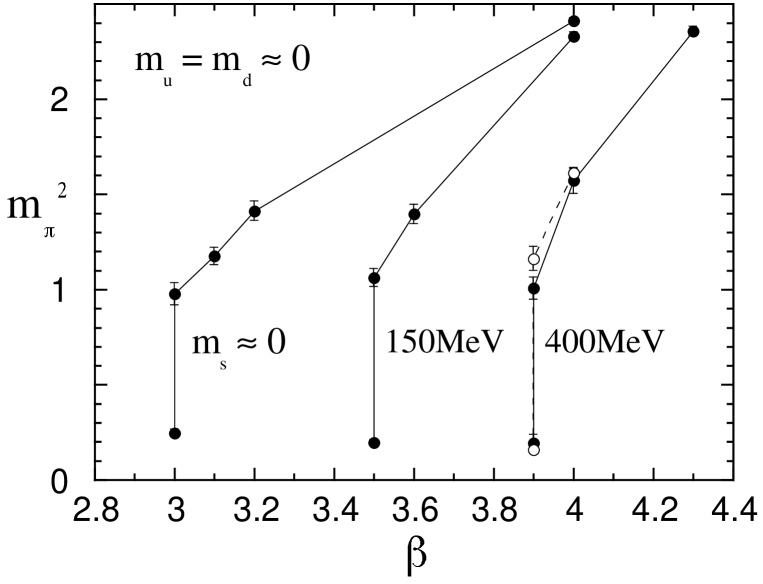
Figure 22: $m_{\pi}^{2}a^{2}$ versus $\beta$ for $m_{s}\simeq 0$, 150 and 400 MeV with $m_{ud}\simeq 0$. Filled and open symbols are for $8^{2}\times 10\times 4$ and $12^{3}\times 4$ lattices, respectively.

The simulation time history of $N_{\rm inv}$ on the $8^{2}\times 10$ spatial lattice is plotted in Fig. 20(a) for the case of 150 MeV. When $\beta\geq 3.6$, $N_{\rm inv}$ is of order of several hundreds, while when $\beta\leq 3.4$, $N_{\rm inv}$ shows a rapid increase with $\tau$. At $\beta=3.5$ we see a clear two-state signal depending on the initial condition: For a hot start, $N_{\rm inv}$ is quite stable around 900 and $m_{\pi}^{2}$ is large ($\sim 1.0$ in lattice units). On the other hand, for a mix start, $N_{\rm inv}$ shows a rapid increase with $\tau$ and exceeds 2,500 in $\tau\sim 10$, and in accord with this, the plaquette and $m_{\pi}^{2}$ decreases with $\tau$ as shown in Fig. 20(b) for the plaquette. For the case of 400 MeV a similar clear two-state signal is observed at $\beta=3.9$ both on the $8^{2}\times 10$ and $12^{3}$ spatial lattices (cf. Fig. 21). The values of $m_{\pi}^{2}$ versus $\beta$ are plotted in Fig. 22 together with those in the case of degenerate $N_{F}=3$ on the $K_{c}$ line. At $\beta=3.5$ for the case of 150 MeV and at $\beta=3.9$ for the case of 400 MeV, we have two values for $m_{\pi}^{2}$ depending on the initial configuration. The larger ones of order 1.0 are for hot starts, while the smaller ones are upper bounds for mix starts. These results imply that $m_{s}^{*}\mathop{\vtop{\halign{#\cr$\hfil\displaystyle{>}\hfil$\crcr\kern 0.5pt\nointerlineskip\cr$\sim$\crcr\kern 0.5pt\cr}}}\limits 400\,{\rm MeV}$ in our normalization for quark masses.

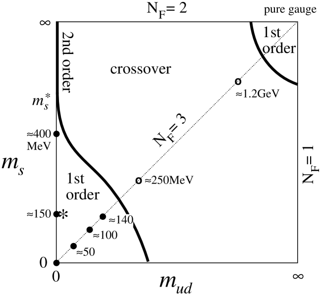
Figure 23: Order of the finite temperature QCD transition in the $(m_{ud},m_{s})$ plane. First order signals are observed at the points marked with filled circle, while no clear two state signals are found at the points with open circle. The second order transition line is suggested [42] to deviate from the vertical axis as $m_{ud}\propto(m_{s}^{*}-m_{s})^{5/2}$ below $m_{s}^{*}$. The values of quark mass in physical units are computed using $a^{-1}$ determined from $m_{\rho}$: $a^{-1}\sim 0.8$ GeV for $\beta\leq 4.7$ and $\sim 1.0(1.8)$ GeV for $\beta=5.0(5.5)$. See Sec. 8 for more detailed discussion on the values of the quark mass in physical units. The real world determined by the value of $m_{\phi}/m_{\rho}$ and $m_{\pi}/m_{\rho}$ corresponds to the point marked with star.

Following the Columbia group [39], we summarize our results about the nature of the QCD transition at $N_{t}=4$ as a function of $m_{ud}$ and $m_{s}$ in Fig. 23, together with theoretical expectations [1, 2, 42] assuming that the chiral transition is of second order for $N_{F}=2$. Clearly the point which corresponds to the physical values of the up, down and strange quark masses measured by $m_{\phi}/m_{\rho}$ and $m_{\pi}/m_{\rho}$ exists in the range of the first order transition. If this situation persists in the continuum limit, the transition for the physical quark masses is of first order.

The Columbia group studied the influence of the strange quark for the case of staggered quarks [39]. Their result shows that no transition occurs at $m_{u}a=m_{d}a=0.025$, $m_{s}a=0.1$ ($m_{u}=m_{d}\sim 12$ MeV, $m_{s}\sim 50$ MeV using $a^{-1}\sim 0.5$ GeV). Their zero-temperature values for $m_{K}/m_{\rho}$ and $m_{\pi}/m_{\rho}$ obtained at this simulation point suggest that this value for $m_{s}$ is smaller than its physical value and those for $m_{u}$ and $m_{d}$ are larger than their physical values. This implies that the transition in the real world is also a crossover, unless the second order transition line, which has a sharp $m_{ud}$ dependence near $m_{s}^{*}$ as shown in Fig. 23 [42], crosses between the physical point and the simulation point.

Although both staggered and Wilson simulations give phase structures qualitatively consistent with theoretical expectations [1, 2, 42], we note that Wilson quarks tend to give larger values for critical quark masses (measured by $m_{\phi}/m_{\rho}$ etc.) than those with staggered quarks. This leads to the difference in the conclusions about the nature of the physical transition. However, since the deviation from the continuum limit is large in both of the studies at $N_{t}=4$, we certainly should make a calculation with larger $N_{t}$ [43] or using an improved action [32] to get closer to the continuum limit and to obtain a definite conclusion about the nature of the QCD transition. With Wilson quarks using the standard gauge action, however, $N_{t}$ should be enormously large ($\geq 18$) [3] in order to avoid the lattice artifacts discussed in Sec. 6. Improvement of the lattice action will be essential especially for Wilson quarks.

9 Conclusions

We have studied the nature of finite temperature transitions near the chiral limit for various numbers of flavors ($N_{F}=2$, 3, and 6) and also for the case of massless up and down quarks and a light strange quark ($N_{F}=2+1$), mainly on lattices with $N_{t}=4$, using the Wilson formalism of quarks on the lattice.

We have found that the chiral transition is continuous (second order or crossover) for $N_{F}=2$, while it is of first order for $N_{F}=3$ and 6. These results are in accordance with theoretical predictions based on universality [1, 2]. Our results with Wilson quarks are also consistent with those with staggered quarks [44].

Our results for QCD with a strange quark as well as up and down quarks obtained on $N_{t}=4$ lattices are summarized in Fig. 23. Clearly, the point which corresponds to the physical values of the up, down and strange quark masses measured by $m_{\phi}/m_{\rho}$ and $m_{\pi}/m_{\rho}$, marked with star in Fig. 23, exists in the range of first order transition. If this situation persists in the continuum limit, the transition for the physical quark masses is of first order.

We have found that Wilson quarks tend to give larger values for critical quark masses (measured, for example, by $m_{\phi}/m_{\rho}$ and $m_{\pi}/m_{\rho}$ ) than those with staggered quarks. This leads to the difference in the conclusions about the nature of the physical transition. Because the deviation from the continuum limit is large on the $N_{t}=4$ lattices, we certainly should make a calculation with larger $N_{t}$ or with an improved action [32] in order to get closer to the continuum limit and to obtain a definite conclusion about the nature of the physical QCD transition, by resolving the discrepancy between Wilson and staggered quarks for the conclusions. Studies with an improved gauge action and the Wilson quark action are in progress.

$\beta$	$K$	$\Delta\tau$	$\tau_{\rm tot}$	$\tau_{\rm therm}$	algo.	$N_{\rm inv}$	phase
0	0.2	0.02	1132	500	H-CR	37	c
0	0.21	0.01	1005	500	H-CR	48	c
0	0.22	0.01	1041	500	H-CR	45	c
0	0.23	0.01	700	500	H-CR	95	c
3	0.18	0.01	250	100	H-CR	37	c
3	0.19	0.01	150	100	H-CR	35	c
3	0.2	0.01	160	100	H-CR	48	c
3.5	0.175	0.01	160	100	H-CR	27	c
3.5	0.185	0.01	160	100	H-CR	34	c
3.5	0.195	0.01	160	100	H-CR	46	c
4	0.17	0.02	1650	500	H-CR	15	c
4	0.18	0.02	2188	1000	H-CR	18	c
4	0.19	0.02	1550	500	H-CR	23	c
4	0.2226	0.002	50	24	H-CG	1054	d
4.1	0.2211	0.005	92	50	H-CG	781	d
4.2	0.2195	0.005	206	100	H-CG	430	d

Table 1: Table of job parameters for $N_{F}=2$ simulations performed on an $8^{2}\times 10\times 4$ lattice. Data marked with † are taken from our previous simulation [13] performed on an $8^{2}\times 20\times 4$ lattice. The column “algo.” is for the algorithm used for update (HMC or R) and for quark matrix inversion (CR or CG). $N_{\rm inv}$ is an average number of iterations needed for the quark matrix inversion. Errors for $N_{\rm inv}$ are in most cases about 1%. The last column is for the initial and final phases (c: the low temperature confining phase, d: the high temperature deconfining phase, and m: mix state), where parentheses mean that the system is not completely thermalized.

$\beta$	$K$	$\Delta\tau$	$\tau_{\rm tot}$	$\tau_{\rm therm}$	algo.	$N_{\rm inv}$	phase
4.3	0.165	0.02	520	320	H-CR	23	c
4.3	0.175	0.01	490	290	H-CR	28	c
4.3	0.185	0.01	400	200	H-CR	39	c
4.3	0.205	0.008	460	250	H-CR	250	d$\rightarrow$c
4.3	0.207	0.005	16		H-CG		c
4.3	0.207	0.005	30		H-CG		d$\rightarrow$(c)
4.3	0.208	0.005	38		H-CG		c
4.3	0.208	0.005	45		H-CG		d$\rightarrow$(c)
4.3	0.21	0.005	150	50	H-CG	820	d
4.3	0.218	0.01	196	100	H-CG	338	d
4.5	0.16	0.02	500	300	H-CR	25	c
4.5	0.17	0.01	580	300	H-CR	34	c
4.5	0.18	0.01	530	300	H-CR	42	c
4.5	0.195	0.01	310	100	H-CR	92	c
4.5	0.2	0.005	175	135	H-CR	280	c
4.5	0.202	0.008	700	300	H-CG	473	d
4.5	0.205	0.01	190	100	H-CG	314	d
4.5	0.2143	0.01	197	100	H-CG	209	d
5	0.14	0.02	500	300	H-CR	17	c
5	0.15	0.02	520	300	H-CR	20	c
5	0.16	0.02	600	300	H-CR	24	c
5	0.17	0.01	540	300	H-CR	41	d$\rightarrow$c
5	0.18	0.01	640	200	H-CG	169	c$\rightarrow$d
5	0.19	0.01	720	300	H-CG	132	d
5	0.1982	0.01	761	300	H-CG	118	c$\rightarrow$d

Table 1: Continued.

$\beta$	$K$	$\Delta\tau$	$\tau_{\rm tot}$	$\tau_{\rm therm}$	algo.	$N_{\rm inv}$	phase
5.25	0.1	0.01	520	300	H-CR	12	c
5.25	0.11	0.01	600	300	H-CR	13	c
5.25	0.12	0.01	600	300	H-CR	15	c
5.25	0.13	0.01	560	300	H-CR	17	c
5.25	0.14	0.01	580	300	H-CR	20	c
5.25	0.15	0.01	520	300	H-CR	25	c
5.25	0.155	0.01	520	300	H-CR	31	d$\rightarrow$c
5.25	0.16	0.01	540	300	H-CR	39	d$\rightarrow$c
5.25	0.165	0.01	600	300	H-CG	121	d
5.25	0.175	0.01	610	300	H-CG	118	d
5.25	0.18	0.01	640	300	H-CG	111	d
5.5†	0.15	0.025	2500	800	H-CR	17	d
5.5†	0.16	0.025	1572	500	H-CR	37	d
5.5†	0.1615	0.025	1532	500	H-CR	43	d
5.5†	0.163	0.025	1458	500	H-CR	53	d
6	0.15	0.01	427	200	H-CG	73	d
6	0.1524	0.01	230	150	H-CG	78	d
6	0.155	0.01	427	200	H-CG	80	d
6	0.16	0.01	400	200	H-CG	83	d
10	0.13	0.01	351	200	H-CG	48	d
10	0.14	0.01	400	200	H-CG	78	d
10	0.15	0.01	338	200	H-CG	60	d

Table 1: Continued.

$\beta$	$K$	$\Delta\tau$	$\tau_{\rm tot}$	$\tau_{\rm therm}$	algo.	$N_{\rm inv}$	phase
4.2	0.2195	0.00125	56	30	H-CG	1119	d
4.3	0.2183	0.002	138	40	H-CG	863	d
4.4	0.2163	0.005	160	30	H-CG	678	d
4.5	0.2143	0.008	130	80	H-CG	505	d
5	0.1982	0.01	224	100	H-CG	160	d
5.02	0.16	0.01	560	300	H-CR	27	c
5.02	0.17	0.01	560	300	H-CR	36	c
5.02	0.18	0.01	180	100	H-CG	143	c
5.02	0.18	0.01	210	100	H-CG	529	d

Table 2: The same as Table 1 for $N_{F}=2$ simulations performed on a $12^{3}\times 6$ lattice.

$\beta$	$K$	$\Delta\tau$	$\tau_{\rm tot}$	$\tau_{\rm therm}$	algo.	$N_{\rm inv}$	phase
4.5	0.16	0.02	500	300	H-CR	23	c
4.5	0.17	0.01	540	300	H-CR	29	c
4.5	0.18	0.01	540	300	H-CR	35	c
5.5†	0.15	0.025	2050	1000	H-CR	8	c
5.5†	0.155	0.02	1600	500	H-CR	23	c
6	0.1524	0.01	230	150	H-CG	78	d

Table 3: The same as Table 1 for $N_{F}=2$ on an $8^{3}\times 10$ lattice. Data marked with † are taken from Ref. [13] obtained on an $8^{3}\times 20$ lattice.

$\beta$	$K$	$\Delta\tau$	$\tau_{\rm tot}$	$\tau_{\rm therm}$	algo.	$N_{\rm inv}$	phase
2.5	0.2381	0.01	8		R-CG	$\sim$2300	d$\rightarrow$(c)
2.7	0.2369	0.01	10		R-CG	$\sim$2300	d$\rightarrow$(c)
2.8	0.2364	0.01	12		R-CG	$>$1900	d$\rightarrow$(c)
2.9	0.2358	0.01	28		R-CG	$\sim$2300	d$\rightarrow$(c)
3	0.205	0.01	280	170	R-CR	64	c
3	0.205	0.01	202	100	R-CR	64	c
3	0.215	0.01	190	100	R-CR	117	c
3	0.225	0.005	75		R-CR	$\sim$563	d$\rightarrow$(c)
3	0.23	0.0025	18		R-CG		d$\rightarrow$(c)
3	0.2352	0.01	23		R-CG	$\sim$2300	m$\rightarrow$(c)
3	0.2352	0.01	68		R-CG	$\sim$2300	c$\rightarrow$(c)
3	0.2352	0.01	159	100	R-CG	851	d
3.1	0.2341	0.01	160	50	R-CG	650	d
3.2	0.2329	0.01	114	50	R-CG	556	d
3.2	0.2329	0.01	169	100	R-CG	504	d
4	0.18	0.01	520	300	R-CR	35	c
4	0.19	0.01	520	300	R-CR	47	c
4	0.2	0.01	391	200	R-CR	84	d$\rightarrow$c
4	0.205	0.01	320	200	R-CG	351	d
4	0.21	0.01	308	200	R-CG	247	d
4	0.2226	0.01	320	200	R-CG	188	d
4.5	0.16	0.01	500	300	R-CR	25	c
4.5	0.17	0.01	542	300	R-CR	30	c
4.5	0.18	0.01	545	300	R-CR	40	d$\rightarrow$c
4.5	0.185	0.01	534	300	R-CR	51	d$\rightarrow$c
4.5	0.186	0.01	301	150	R-CR	56	c
4.5	0.1875	0.01	191	100	R-CR	82	c
4.5	0.1875	0.01	181	100	R-CG	248	d
4.5	0.189	0.01	207	100	R-CG	214	d

Table 4: The same as Table 1 for $N_{F}=3$ on an $8^{2}\times 10\times 4$ lattice.

$\beta$	$K$	$\Delta\tau$	$\tau_{\rm tot}$	$\tau_{\rm therm}$	algo.	$N_{\rm inv}$	phase
4.5	0.19	0.01	336	200	R-CG	200	d
4.5	0.2	0.01	394	200	R-CG	158	d
4.5	0.205	0.01	190		R-CG	142	d
4.5	0.2143	0.01	101		R-CG	132	d
5	0.13	0.01	313	150	R-CR	49	c
5	0.14	0.01	275	150	R-CR	20	c
5	0.15	0.01	310	150	R-CR	22	c
5	0.16	0.01	324	150	R-CR	27	c
5	0.165	0.01	373	150	R-CR	65	c
5	0.165	0.01	202	150	R-CG	48	d$\rightarrow$c
5	0.166	0.01	120		R-CG		d$\rightarrow$(c)
5	0.166	0.01	264	150	R-CR	35	c
5	0.167	0.01	145		R-CR		c$\rightarrow$(d)
5	0.167	0.01	187	100	R-CG	155	d
5	0.17	0.01	291	150	R-CG	119	d
5.5	0.1	0.01	652	150	R-CR	13	c
5.5	0.11	0.01	505	150	R-CR	15	c
5.5	0.12	0.01	571	250	R-CR	16	c
5.5	0.125	0.01	695	250	R-CR	17	c$\rightarrow$m
5.5	0.1275	0.01	676	100	R-CR	18	d
5.5	0.13	0.01	364	150	R-CR	18	c$\rightarrow$d
5.5	0.135	0.01	174	100	R-CR	20	d$\rightarrow$d
5.5	0.14	0.01	296	100	R-CR	23	d
6	0.08	0.01	355	100	R-CG	23	d
6	0.09	0.01	194	100	R-CG	27	d
6	0.1	0.01	320	100	R-CG	33	d
6	0.11	0.01	270	100	R-CG	41	d
6	0.12	0.01	244	100	R-CG	51	d
6	0.135	0.01	180	100	R-CG	72	d

Table 4: Continued.

$\beta$	$K$	$\Delta\tau$	$\tau_{\rm tot}$	$\tau_{\rm therm}$	algo.	$N_{\rm inv}$	phase
4	0.2	0.01	198	100	R-CR	82	c
4	0.202	0.01	273	100	R-CR	101	c
4	0.203	0.01	229	100	R-CR	117	c
4	0.203	0.01	63		R-CG		d$\rightarrow$(c)
4	0.204	0.01	219	100	R-CG	152	c
4	0.204	0.01	169	100	R-CG	449	d
4	0.205	0.01	93		R-CG		c$\rightarrow$(d)
4	0.205	0.01	192	100	R-CG	380	d
4	0.21	0.01	203	100	R-CG	272	d
4.5	0.18	0.01	282	100	R-CR	40	c
4.5	0.186	0.01	230	100	R-CR	56	c
4.5	0.1875	0.01	1040	369	R-CR	74	c
4.5	0.1875	0.01	1072	100	R-CG	264	d
4.5	0.189	0.01	183	100	R-CG	230	d
4.5	0.19	0.01	196	100	R-CG	219	d
4.7	0.17	0.01	307	100	R-CR	32	c
4.7	0.175	0.01	225	100	R-CR	38	c
4.7	0.178	0.01	232	100	R-CG	117	d$\rightarrow$c
4.7	0.179	0.01	335	100	R-CR	48	c
4.7	0.179	0.01	253		R-CG		d$\rightarrow$(c)
4.7	0.1795	0.01	1035	100	R-CR	50	c
4.7	0.1795	0.01	1073	100	R-CG	236	d
4.7	0.18	0.01	299	100	R-CG	228	d
4.7	0.18	0.01	410		R-CG		c$\rightarrow$(d)

Table 5: The same as Table 1 for $N_{F}=3$ on a $12^{3}\times 4$ lattice.

$\beta$	$K$	$\Delta\tau$	$\tau_{\rm tot}$	$\tau_{\rm therm}$	algo.	$N_{\rm inv}$	phase
5	0.165	0.01	203	100	R-CR	33	c
5	0.166	0.01	574	200	R-CR	35	c
5	0.166	0.01	405		R-CG/CR		d$\rightarrow$(c)
5	0.16625	0.01	570	200	R-CR	37	c$\rightarrow$m
5	0.16625	0.01	545	200	R-CR	47	d$\rightarrow$m
5	0.1665	0.01	502		R-CR		c$\rightarrow$(d)
5	0.1665	0.01	611	200	R-CR	75	d
5	0.167	0.01	475	250	R-CR	53	d
5	0.168	0.01	419	100	R-CR	104	d
5	0.169	0.01	164	100	R-CG	163	d
5	0.17	0.01	231	100	R-CG	166	d

Table 5: Continued.

$\beta$	$K$	$\Delta\tau$	$\tau_{\rm tot}$	$\tau_{\rm therm}$	algo.	$N_{\rm inv}$	phase
0	0.2	0.01	32	20	R-CR	38	c
0	0.21	0.01	32	20	R-CR	49	c
0	0.22	0.01	33	18	R-CR	67	c
0	0.235	0.01	40	20	R-CR	155	c
0.1	0.2495	0.01	11		R-CG	$>$5000	d$\rightarrow$(c)
0.2	0.249	0.01	11		R-CG	$>$5000	d$\rightarrow$(c)
0.2	0.24936	0.01	23		R-CG	$>$10000	d$\rightarrow$(c)
0.3	0.2485	0.01	16		R-CG	$>$5000	m$\rightarrow$(c)
0.3	0.2485	0.01	9		R-CG	$>$5000	m$\rightarrow$(c)
0.3	0.2485	0.01	27		R-CG	600	d
0.3	0.249	0.01	16			$>$5000	m$\rightarrow$(c)
0.4	0.248	0.01	20	10	R-CG	500	d
0.5	0.23	0.01	6		R-CG		d$\rightarrow$(c)
0.5	0.235	0.01	6		R-CG		d$\rightarrow$(c)
0.5	0.24	0.01	6		R-CG		d$\rightarrow$(c)
0.5	0.245	0.01	53		R-CG	$\sim$1400	d$\rightarrow$c
0.5	0.2475	0.01	25	15	R-CG	445	d
1	0.2	0.01	113	50	R-CR	42	c
1	0.21	0.01	104	50	R-CR	60	c
1	0.22	0.01	115	55	R-CR	80	c
1	0.225	0.01	267	100	R-CR	126	c
1	0.23	0.01	293	100	R-CR	192	c
1	0.235	0.01	40		R-CG		d$\rightarrow$c
1	0.235	0.005	112	60	R-CG	970	c
1	0.235	0.005	19		R-CG		d$\rightarrow$(c)
1	0.237	0.005	42		R-CG		d
1	0.237	0.005	49		R-CG		c$\rightarrow$(d)
1	0.238	0.005	28		R-CG	440	d
1	0.24	0.005	108	40	R-CG	325	d
1	0.245	0.01	114	60	R-CG	306	d

Table 6: The same as Table 1 for $N_{F}=6$ on an $8^{2}\times 10\times 4$ lattice.

$\beta$	$K$	$\Delta\tau$	$\tau_{\rm tot}$	$\tau_{\rm therm}$	algo.	$N_{\rm inv}$	phase
2	0.24	0.01	18		R-CG	162	d
4	0.22	0.01	15		R-CG	88	d
4.5	0.15	0.01	71	61	R-CR	21	c
4.5	0.16	0.01	38	28	R-CR	27	c
4.5	0.165	0.01	60	50	R-CR	32	c
4.5	0.165	0.01	60		R-CR		d$\rightarrow$(c)
4.5	0.166	0.01	277	267	R-CR	36	d$\rightarrow$c
4.5	0.167	0.01	193	183	R-CR	36	c
4.5	0.167	0.01	159	149	R-CR	105	d
4.5	0.168	0.01	152		R-CG		c$\rightarrow$(d)
4.5	0.17	0.01	73		R-CG		c$\rightarrow$(d)
4.5	0.18	0.01	41	31	R-CG	115	c$\rightarrow$d
4.5	0.19	0.01	38	28	R-CG	92	c$\rightarrow$d
4.5	0.2143	0.01	181	150	R-CG	87	d

Table 6: Continued.

$\beta$	$K_{ud}$	$K_{s}$	$\tau_{\rm tot}$	$\tau_{\rm therm}$	$N_{\rm inv}^{ud}$	$N_{\rm inv}^{s}$	phase
3.2	0.2329	0.2043	15		$\sim$3000	$\sim$250	d$\rightarrow$(c)
3.4	0.2306	0.2026	20		$\sim$3000	$\sim$290	d$\rightarrow$(c)
3.5	0.2295	0.2017	9		$\sim$3000	$\sim$260	m$\rightarrow$(c)
3.5	0.2295	0.2017	553	100	862	394	d
3.6	0.2281	0.2006	153	100	622	344	d
3.7	0.2267	0.1692	20		$\sim$2500	$\sim$100	d$\rightarrow$(c)
3.8	0.2254	0.1684	47		$\sim$2500	$\sim$93	d$\rightarrow$(c)
3.9	0.224	0.1677	12		$\sim$2500	$\sim$93	m$\rightarrow$(c)
3.9	0.224	0.1677	760	100	797	135	d
4	0.2226	0.1669	159	100	521	137	d
4	0.2226	0.1964	167	100	235	201	d
4.3	0.218	0.1643	159	100	229	130	d
5.5	0.163	0.15	376	208	119	97	d

Table 7: The same as Table 1 for $N_{F}=2+1$ on an $8^{2}\times 10\times 4$ lattice. The molecular dynamics time step is $\Delta\tau=0.01$. Simulations are performed with the R algorithm for updating configurations and with the CG method for quark matrix inversions.

$\beta$	$K_{ud}$	$K_{s}$	$\tau_{\rm tot}$	$\tau_{\rm therm}$	$N_{\rm inv}^{ud}$	$N_{\rm inv}^{s}$	phase
3.9	0.224	0.1677	14		$\sim$3000	$\sim$93	m$\rightarrow$(c)
3.9	0.224	0.1677	398	100	999	139	d
4	0.2226	0.1669	396	100	636	141	d

Table 8: The same as Table 7 for $N_{F}=2+1$ on an $8^{2}\times 10\times 4$ lattice. Simulations are performed with the R algorithm for updating configurations and with the CG method for quark matrix inversions.

$\beta$	$K_{ud}$	$K_{s}$	$\tau_{\rm tot}$	$\tau_{\rm therm}$	$N_{\rm inv}^{ud}$	$N_{\rm inv}^{s}$	phase
3.5	0.195	0.2017	196	100	46	58	c
3.5	0.2	0.2017	164	50	57	59	c
3.5	0.205	0.2017	166	50	74	61	c
3.5	0.21	0.2017	158	40	109	64	c

Table 9: The same as Table 7 for $N_{F}=2+1$ on an $8^{3}\times 10$ lattice. Simulations are performed with the R algorithm for updating configurations and with the CR method for quark matrix inversions.

$\beta$	$K_{c}(m_{\pi}^{2})$	$K_{c}(m_{q})$
3.0	0.235(1)	0.230(1)
3.5	0.230(1)	0.226(1)
4.0	0.223(1)	0.218(4)
4.3	0.218(1)	0.214(1)
4.5	0.214(1)	0.210(1)
6.0		0.1564(1)
10.0		0.1396(1)

Table 10: The chiral limit $K_{c}$ for $N_{F}=2$ determined on an $8^{2}\times 10\times 4$ lattice. The results for $\beta=3.0$ — 4.5 are determined by $m_{\pi}=0$ and $m_{q}=0$, where values of $m_{\pi}^{2}$ and $m_{q}$ in the confining phase are linearly extrapolated in $1/K$. The results for $\beta=6.0$ and 10.0 are determined from an interpolation of $m_{q}$ in the deconfining phase.

	$N_{t}=4$		$N_{t}=8$
$N_{F}$	$K_{c}(m_{\pi}^{2})$	$K_{c}(m_{q})$	$K_{c}(m_{\pi}^{2})$	$K_{c}(m_{q})$
2	0.214(1)	0.210(1)	0.212(1)	0.209(1)
3	0.210(1)	0.204(1)
6	0.205(2)	0.200(1)

Table 11: The chiral limit $K_{c}$ at $\beta=4.5$ determined by $m_{\pi}=0$ and $m_{q}=0$, where values of $m_{\pi}^{2}$ and $m_{q}$ in the confining phase are linearly extrapolated in $1/K$ using data from $K=0.16$ — 0.18 for $N_{F}=2$ and 3 and $K=0.15$ — 0.165 for $N_{F}=6$ (because $K_{t}=0.167(1)$ for $N_{F}=6$ at $N_{t}=4$). The spatial lattice size is $8^{2}\times 10$.

$N_{F}=2$		$N_{F}=3$		$N_{F}=6$
$\beta$	$K_{t}$	$\beta$	$K_{t}$	$\beta$	$K_{t}$
4.3	0.207–0.210	3.0	$>$ 0.230	0.5	0.245–0.2475
4.5	0.200–0.202	4.0	0.200–0.205	1.0	0.235–0.237
5.0	0.170–0.180	4.5	0.186–0.189	4.5	0.166–0.168
5.25	0.160–0.165	4.5*	0.186–0.189
		4.7*	0.179–0.180
		5.0	0.166–0.167
		5.0*	0.166–0.1665
		5.5	0.125–0.130

Table 12: Finite temperature transition $K_{t}$ for $N_{F}=2$, 3 and 6 obtained on an $8^{2}\times 10\times 4$ lattice (data with * obtained on a $12^{3}\times 4$ lattice). For $N_{F}=2$ at $\beta=5.0$, the data by the MILC collaboration [16] give a more precise value 0.177 — 0.178 for $K_{t}$ (cf. Fig. 3).

$\beta$	$K$	plaquette	Polyakov	$m_{\pi}a$	$2m_{q}a$	$m_{\rho}a$
0	0.2	0.0088(1)	0.0367(3)	1.441(3)	0.715(2)	1.542(25)
0	0.21	0.0109(1)	0.0449(3)	1.272(4)	0.552(3)	1.405(34)
0	0.22	0.0134(1)	0.0548(32)	1.086(3)	0.400(2)	1.300(37)
0	0.23	0.0161(2)	0.0681(10)	0.871(5)	0.253(2)	1.074(65)
3	0.18	0.2174(3)	0.0252(13)	1.554(7)	0.808(5)	1.631(44)
3	0.19	0.2201(2)	0.0361(7)	1.376(7)	0.621(5)	1.473(48)
3	0.2	0.2247(3)	0.0454(14)	1.179(5)	0.437(3)	1.342(61)
3.5	0.175	0.2587(3)	0.0268(12)	1.606(5)	0.848(5)	1.679(24)
3.5	0.185	0.2624(3)	0.0333(13)	1.408(7)	0.649(4)	1.532(31)
3.5	0.195	0.267(4)	0.0436(13)	1.211(7)	0.461(4)	1.392(43)
4	0.17	0.3034(1)	0.0249(2)	1.623(3)	0.874(2)	1.688(5)
4	0.18	0.3079(1)	0.0318(2)	1.426(3)	0.659(2)	1.523(6)
4	0.19	0.3141(1)	0.0408(2)	1.207(4)	0.458(2)	1.367(14)
4	0.2226	0.4002(7)	0.1328(24)	0.831(35)	-.074(11)
4.1	0.2211	0.4300(4)	0.1345(20)	0.997(41)	-.100(9)	1.07(44)
4.2	0.2195	0.4445(6)	0.1535(29)	1.254(32)	-.081(9)	2.12(36)
4.3	0.165	0.3319(2)	0.0220(7)	1.663(7)	0.920(5)	1.715(21)
4.3	0.175	0.3367(2)	0.0293(8)	1.463(7)	0.696(5)	1.546(22)
4.3	0.185	0.3440(2)	0.0404(8)	1.242(6)	0.485(3)	1.379(24)
4.3	0.205	0.3732(3)	0.0736(8)	0.647(8)	0.094(3)
4.3	0.21	0.4286(4)	0.1369(12)	0.755(74)	-.026(9)
4.3	0.218	0.4661(4)	0.1790(18)	1.413(13)	-.083(9)	1.784(55)
4.5	0.16	0.3524(2)	0.0209(7)	1.732(6)	0.997(4)	1.782(8)
4.5	0.17	0.3580(2)	0.0282(6)	1.520(6)	0.760(4)	1.595(1)
4.5	0.18	0.3656(2)	0.0384(7)	1.298(5)	0.534(4)	1.423(8)
4.5	0.195	0.3856(3)	0.0590(9)	0.882(11)	0.201(4)	1.145(38)
4.5	0.2	0.4007(6)	0.0807(19)	0.696(24)	0.090(5)

Table 13: Results of the plaquette, the Polyakov loop, the pion screening mass, twice the quark mass, and the rho meson screening mass for $N_{F}=2$ obtained on an $8^{2}\times 10\times 4$ lattice. Data marked with † are taken from Ref. [13] obtained on an $8^{2}\times 20\times 4$ lattice.

$\beta$	$K$	plaquette	Polyakov	$m_{\pi}a$	$2m_{q}a$	$m_{\rho}a$
4.5	0.202	0.4591(3)	0.1643(9)	1.135(36)	-.072(8)
4.5	0.205	0.4752(3)	0.1809(17)	1.421(18)	-.128(27)	1.738(43)
4.5	0.2143	0.4949(3)	0.2137(16)	1.552(10)	-.034(8)	1.746(19)
5	0.14	0.4095(2)	0.0128(7)	2.046(5)	1.379(5)	2.072(6)
5	0.15	0.4148(2)	0.0217(7)	1.801(12)	1.093(1)	1.828(19)
5	0.16	0.4215(2)	0.0301(7)	1.551(8)	0.805(6)	1.604(1)
5	0.17	0.4351(2)	0.0409(8)	1.279(6)	0.522(5)	1.394(12)
5	0.18	0.5174(2)	0.2250(8)	1.430(13)	-.086(9)	1.637(11)
5	0.19	0.5378(1)	0.2580(7)	1.686(11)	-.096(8)	1.861(8)
5	0.1982	0.5473(1)	0.2789(6)	1.717(5)	0.029(5)	1.837(7)
5.25	0.1	0.4426(2)	0.0018(8)	2.934(5)	2.508(5)	2.937(6)
5.25	0.11	0.4446(2)	0.0041(5)	2.681(10)	2.191(8)	2.687(11)
5.25	0.12	0.4472(2)	0.0085(7)	2.423(7)	1.867(7)	2.433(8)
5.25	0.13	0.4502(2)	0.0140(7)	2.184(8)	1.563(6)	2.200(9)
5.25	0.14	0.4556(2)	0.0213(7)	1.941(4)	1.263(4)	1.970(5)
5.25	0.15	0.4635(3)	0.0305(9)	1.657(12)	0.939(9)	1.709(14)
5.25	0.155	0.4746(3)	0.0499(12)	1.495(6)	0.756(6)	1.563(7)
5.25	0.16	0.4846(3)	0.0678(11)	1.324(9)	0.570(7)	1.397(12)
5.25	0.165	0.5307(2)	0.2241(10)	1.351(9)	0.173(9)	1.468(12)
5.25	0.175	0.5513(2)	0.2695(8)	1.531(12)	-.136(18)	1.696(10)
5.25	0.18	0.5589(1)	0.2861(8)	1.696(6)	-.160(6)	1.853(7)
5.5†	0.15	0.5530(2)	0.2413(7)	1.486(6)	0.512(1)	1.528(8)
5.5†	0.16	0.5662(2)	0.2815(5)	1.415(7)	0.103(5)	1.490(7)
5.5†	0.1615	0.5677(2)	0.2863(8)	1.441(5)	0.048(6)	1.513(9)
5.5†	0.163	0.5699(1)	0.2905(8)	1.438(8)	-.016(4)	1.506(8)
6	0.15	0.6122(2)	0.3456(10)	1.469(7)	0.233(5)	1.510(8)
6	0.1524	0.6131(3)	0.3478(16)	1.467(7)	0.142(8)	1.514(7)
6	0.155	0.6157(2)	0.3555(9)	1.480(5)	0.042(7)	1.529(9)
6	0.16	0.6188(2)	0.3607(9)	1.534(6)	-.120(6)	1.594(8)
10	0.13	0.7853(1)	0.6126(11)	1.496(6)	0.447(2)	1.491(6)
10	0.14	0.7865(1)	0.6157(8)	1.439(8)	-.010(4)	1.437(9)
10	0.15	0.7873(1)	0.6230(8)	1.591(2)	-.427(6)	1.598(3)

Table 13: Continued.

$\beta$	$K$	plaquette	Polyakov	$m_{\pi}a$	$2m_{q}a$	$m_{\rho}a$
4.2	0.2195	0.4410(3)	0.0067(12)	0.897(50)	-.082(11)
4.3	0.2183	0.4593(2)	0.0054(6)	1.070(62)	-.111(21)
4.4	0.2163	0.4742(1)	0.0098(7)	1.241(28)	-.105(8)	1.677(52)
4.5	0.2143	0.4889(2)	0.0071(10)	1.371(11)	-.058(9)	1.604(31)
5	0.1982	0.5455(1)	0.0831(10)	1.638(7)	0.044(9)	1.749(8)
5.02	0.16	0.4256(1)	0.0023(4)	1.542(5)	0.800(4)	1.605(6)
5.02	0.17	0.4384(1)	0.0041(3)	1.242(6)	0.508(4)	1.343(11)
5.02	0.18c	0.4696(1)	0.0102(5)	0.710(10)	0.149(5)	0.986(29)
5.02	0.18d	0.5180(2)	0.0399(9)	0.923(47)	-.164(18)	1.40(16)

Table 14: The same as Table 13 for $N_{F}=2$ on a $12^{3}\times 6$ lattice.

$\beta$	$K$	plaquette	Polyakov	$m_{\pi}a$	$2m_{q}a$	$m_{\rho}a$
4.5	0.16	0.3522(1)	0.0010(7)	1.731(7)	0.999(5)	1.779(20)
4.5	0.17	0.3574(1)	0.0004(6)	1.513(5)	0.759(4)	1.588(19)
4.5	0.18	0.3649(1)	0.0023(6)	1.281(5)	0.529(3)	1.398(18)
5.5†	0.15	0.5377(3)	0.0073(1)	1.115(16)	0.542(6)	1.167(19)
5.5†	0.155	0.5481(3)	0.0081(2)	0.807(35)	0.308(14)	0.874(39)
6	0.1524	0.6131(3)	0.3478(16)	0.837(19)	-.003(4)	0.881(22)

Table 15: The same as Table 13 for $N_{F}=2$ on an $8^{3}\times 10$ lattice. Data marked with † are taken from Ref. [13] obtained on an $8^{3}\times 20$ lattice.

$\beta$	$K$	plaquette	Polyakov	$m_{\pi}a$	$2m_{q}a$	$m_{\rho}a$
3	0.205	0.2402(2)	0.0779(7)	1.049(4)	0.334(2)	1.223(18)
3	0.215	0.2501(3)	0.1002(12)	0.820(4)	0.180(1)	1.247(67)
3	0.225	0.2635(6)	0.1266(24)
3	0.2352d	0.3546(6)	0.1718(16)	0.988(30)	-.066(5)
3.1	0.2341	0.3743(3)	0.1812(12)	1.084(21)	-.069(4)	1.53(26)
3.2	0.2329	0.3889(2)	0.1850(10)	1.192(19)	-.077(7)	1.52(22)
4	0.18	0.3176(2)	0.0508(7)	1.405(7)	0.638(5)	1.497(14)
4	0.19	0.3297(2)	0.0669(7)	1.179(8)	0.424(5)	1.346(17)
4	0.2	0.3486(3)	0.0978(8)	0.899(9)	0.206(5)	1.193(50)
4	0.205	0.4465(5)	0.2102(11)	1.313(4)	-.056(30)	1.77(18)
4	0.21	0.4674(3)	0.2341(11)	1.542(10)	-.057(11)	1.760(20)
4	0.2226	0.4944(2)	0.2637(12)	1.552(5)	0.009(4)	1.689(6)
4.5	0.16	0.3598(2)	0.0334(7)	1.717(5)	0.979(5)	1.768(6)
4.5	0.17	0.3691(2)	0.0459(6)	1.497(5)	0.732(3)	1.575(9)
4.5	0.18	0.3835(2)	0.0641(7)	1.250(6)	0.478(4)	1.385(14)
4.5	0.185	0.3954(2)	0.0812(8)	1.094(8)	0.340(5)	1.281(15)
4.5	0.186	0.4025(3)	0.0927(10)	1.070(9)	0.299(5)	1.267(23)
4.5	0.1875c	0.4129(6)	0.1094(15)	1.023(6)	0.250(8)	1.287(34)
4.5	0.1875d	0.4867(6)	0.2343(17)	1.394(44)	-.078(7)	1.636(55)
4.5	0.189	0.4964(4)	0.2492(15)	1.502(19)	-.114(14)	1.696(23)
4.5	0.19	0.5012(3)	0.2560(11)	1.580(10)	-.118(12)	1.788(18)
4.5	0.2	0.5232(2)	0.2852(11)	1.693(5)	0.010(6)	1.814(8)
4.5	0.205	0.5318(3)	0.2957(13)
4.5	0.2143	0.5433(4)	0.3183(27)

Table 16: The same as Table 13 for $N_{F}=3$ on an $8^{2}\times 10\times 4$ lattice.

$\beta$	$K$	plaquette	Polyakov	$m_{\pi}a$	$2m_{q}a$	$m_{\rho}a$
5	0.13	0.4102(2)	0.0138(6)	2.257(10)	1.647(76)	2.271(10)
5	0.14	0.4163(2)	0.0223(9)	2.036(7)	1.373(6)	2.063(8)
5	0.15	0.4243(3)	0.0319(9)	1.790(7)	1.077(6)	1.830(10)
5	0.16	0.4382(3)	0.0522(10)	1.515(9)	0.763(8)	1.586(12)
5	0.165	0.4533(3)	0.0798(10)	1.359(12)	0.574(12)	1.444(16)
5	0.166	0.4697(4)	0.1247(17)	1.340(13)	0.491(14)	1.447(12)
5	0.167	0.5141(4)	0.2369(17)	1.379(11)	0.185(17)	1.488(17)
5	0.17	0.5297(3)	0.2698(11)	1.473(10)	0.003(19)	1.586(11)
5.5	0.1	0.5011(2)	0.0185(7)	2.846(5)	2.413(5)	2.849(5)
5.5	0.11	0.5052(3)	0.0283(10)	2.551(7)	2.055(7)	2.557(8)
5.5	0.12	0.5145(3)	0.0516(15)	2.253(9)	1.679(8)	2.262(10)
5.5	0.125	0.5216(3)	0.0837(16)	2.104(4)	1.495(5)	2.116(5)
5.5	0.1275	0.5276(3)	0.1226(16)	2.031(4)	1.392(4)	2.046(4)
5.5	0.13	0.5384(3)	0.1872(13)	1.950(5)	1.254(4)	1.967(6)
5.5	0.135	0.5453(4)	0.2141(24)	1.814(8)	1.056(6)	1.836(8)
5.5	0.14	0.5521(2)	0.2413(13)	1.672(4)	0.843(4)	1.696(5)
6	0.08	0.5963(2)	0.2582(13)	3.312(5)	2.993(4)	3.313(5)
6	0.09	0.5971(3)	0.2745(15)	2.982(5)	2.591(4)	2.984(5)
6	0.1	0.5984(2)	0.2829(13)	2.647(4)	2.182(4)	2.649(4)
6	0.11	0.5987(2)	0.2874(15)	2.344(5)	1.799(4)	2.347(5)
6	0.12	0.6024(2)	0.3063(15)	2.046(11)	1.401(9)	2.051(12)
6	0.135	0.6076(3)	0.3346(16)

Table 16: Continued.

$\beta$	$K$	plaquette	Polyakov	$m_{\pi}a$	$2m_{q}a$	$m_{\rho}a$
4	0.2	0.3479(2)	0.0945(8)	0.910(6)	0.207(3)	1.139(26)
4	0.202	0.3541(2)	0.1053(6)	0.859(4)	0.174(2)	1.129(25)
4	0.203	0.3580(2)	0.1104(7)	0.836(5)	0.154(2)	1.139(30)
4	0.204c	0.3684(2)	0.1270(8)	0.809(9)	0.119(2)	1.077(79)
4	0.204d	0.4378(3)	0.2030(9)
4	0.205	0.4486(2)	0.2102(7)
4	0.21	0.4679(2)	0.2322(8)
4.5	0.18	0.3828(1)	0.0645(5)	1.252(5)	0.479(3)	1.378(9)
4.5	0.186	0.4014(2)	0.0921(7)	1.070(7)	0.304(4)	1.266(12)
4.5	0.1875c	0.4138(2)	0.1115(4)	1.032(6)	0.244(3)	1.257(14)
4.5	0.1875d	0.4870(1)	0.2353(3)	1.430(10)	-.079(5)	1.674(14)
4.5	0.189	0.4945(3)	0.2457(10)	1.556(7)	-.097(7)	1.753(13)
4.5	0.19	0.5007(2)	0.2525(7)	1.586(9)	-.114(7)	1.829(16)
4.7	0.17	0.3986(1)	0.0536(4)	1.417(6)	0.647(5)	1.505(8)
4.7	0.175	0.4076(2)	0.0661(7)	1.286(6)	0.513(4)	1.405(9)
4.7	0.178	0.4185(3)	0.0814(7)	1.190(8)	0.408(4)	1.328(13)
4.7	0.179	0.4234(2)	0.0905(7)	1.147(6)	0.369(3)	1.312(9)
4.7	0.1795c	0.4275(1)	0.0976(3)	1.144(4)	0.350(3)	1.310(7)
4.7	0.1795d	0.4968(1)	0.2360(4)	1.393(7)	-.004(7)	1.597(9)
4.7	0.18	0.4995(3)	0.2399(7)	1.381(15)	0.003(13)	1.596(16)
5	0.165	0.4538(3)	0.0786(10)	1.357(4)	0.569(4)	1.446(5)
5	0.166	0.4630(2)	0.1017(7)	1.318(6)	0.513(3)	1.424(7)
5	0.16625	0.4791(2)	0.1454(7)	1.312(4)	0.428(3)	1.419(6)
5	0.1665	0.5031(2)	0.2086(8)	1.349(6)	0.280(5)	1.463(6)
5	0.167	0.5151(3)	0.2377(8)	1.384(7)	0.178(8)	1.495(9)
5	0.168	0.5193(2)	0.2478(5)	1.401(5)	0.134(5)	1.516(5)
5	0.169	0.5263(2)	0.2609(10)	1.421(17)	0.062(8)	1.537(19)
5	0.17	0.5294(2)	0.2686(8)	1.432(10)	0.020(7)	1.564(9)

Table 17: The same as Table 13 for $N_{F}=3$ on a $12^{3}\times 4$ lattice.

$\beta$	$K$	plaquette	Polyakov	$m_{\pi}a$	$2m_{q}a$	$m_{\rho}a$
0	0.2	0.0286(5)	0.1208(32)	1.422(7)	0.687(2)	1.524(23)
0	0.21	0.0362(6)	0.1567(20)	1.248(4)	0.514(4)	1.384(27)
0	0.22	0.0412(6)	0.1971(32)	1.064(9)	0.360(9)	1.227(47)
0	0.235	0.0566(6)	0.2632(24)	0.777(5)	0.160(1)	1.157(86)
0.3	0.2485d	0.2229(9)	0.3109(19)	1.040(5)	-.037(4)
0.4	0.248	0.2364(12)	0.3112(28)	1.079(16)	-.042(5)
0.5	0.2475	0.2540(8)	0.3060(26)	1.157(6)	-.063(3)
1	0.2	0.0976(3)	0.1313(14)	1.364(4)	0.615(4)	1.494(7)
1	0.21	0.1075(3)	0.1634(12)	1.170(5)	0.438(2)	1.332(15)
1	0.22	0.1197(4)	0.2099(13)	0.984(3)	0.281(2)	1.217(19)
1	0.225	0.1251(2)	0.2385(8)	0.888(4)	0.211(1)	1.201(28)
1	0.23	0.1262(2)	0.2595(7)	0.797(3)	0.154(1)	1.218(47)
1	0.235	0.1633(6)	0.3035(16)	0.725(6)	0.078(2)	1.11(23)
1	0.24	0.2944(5)	0.3032(47)	1.261(7)	-.044(6)	1.586(38)
1	0.245	0.3207(3)	0.2988(15)	1.314(12)	-.058(7)	1.717(82)
4.5	0.15	0.3690(3)	0.0493(17)	1.909(11)	1.200(8)	1.945(34)
4.5	0.16	0.3879(5)	0.0822(23)	1.668(10)	0.908(10)	1.728(41)
4.5	0.165	0.4013(7)	0.1083(33)	1.551(7)	0.765(3)	1.641(36)
4.5	0.166	0.4171(13)	0.1394(29)
4.5	0.167	0.4177(4)	0.1317(18)
4.5	0.167	0.5024(3)	0.3034(30)
4.5	0.168	0.5156(6)	0.3256(26)
4.5	0.17	0.5295(14)	0.3448(28)	1.554(12)	-.041(23)
4.5	0.18	0.5677(4)	0.3964(27)	1.799(5)	-.116(10)
4.5	0.19	0.5889(5)	0.4237(24)	1.803(6)	0.167(7)
4.5	0.2143	0.6202(3)	0.4666(19)	1.616(6)	0.156(10)	1.641(8)

Table 18: The same as Table 13 for $N_{F}=6$ on an $8^{4}\times 10\times 4$ lattice.

$\beta$	$K_{ud}$	$K_{s}$	plaquette	Polyakov	$m_{\pi}a$	$m_{\rho}a$	$m_{\phi}a$
3.5d	0.2295	0.2017	0.3909(2)	0.178(1)	0.991(19)		1.432(33)
3.6	0.2281	0.2006	0.4119(6)	0.189(1)	1.182(21)
3.9d	0.224	0.1677	0.4173(2)	0.170(1)	1.003(29)		1.527(7)
4	0.2226	0.1669	0.4403(5)	0.189(2)	1.254(27)	1.774(93)	1.534(23)
4	0.2226	0.1964	0.4761(4)	0.244(2)	1.526(7)	1.713(6)	1.810(19)
4.3	0.218	0.1643	0.4902(4)	0.246(2)	1.535(8)	1.699(12)	1.520(10)
5.5	0.163	0.15	0.5801(2)	0.328(1)	1.487(10)	1.569(12)	1.532(9)

Table 19: Results of the plaquette, the Polyakov loop, the pion screening mass, the rho meson screening mass, and the phi meson screening mass for $N_{F}=2+1$ obtained on an $8^{2}\times 10\times 4$ lattice.

$\beta$	$K_{ud}$	$K_{s}$	plaquette	Polyakov	$m_{\pi}a$	$m_{\rho}a$	$m_{\phi}a$
3.9d	0.224	0.1677	0.4180(2)	0.169(1)	1.078(29)		1.518(8)
4	0.2226	0.1669	0.4407(1)	0.190(1)	1.270(9)	1.702(54)	1.509(6)

Table 20: The same as Table 19 for $N_{F}=2+1$ obtained on a $12^{3}\times 4$ lattice.

$\beta$	$K_{ud}$	$K_{s}$	plaquette	Polyakov	$m_{\pi}a$	$m_{\rho}a$	$m_{\phi}a$
3.5	0.195	0.2017	0.2814(2)	0.001(1)	1.150(4)	1.305(8)	1.198(10)
3.5	0.2	0.2017	0.2851(2)	0.003(1)	1.023(3)	1.218(12)	1.194(13)
3.5	0.205	0.2017	0.2891(2)	0.003(1)	0.899(4)	1.114(18)	1.172(15)
3.5	0.21	0.2017	0.2935(2)	0.003(1)	0.748(4)	1.084(42)	1.179(16)

Table 21: The same as Table 19 for $N_{F}=2+1$ obtained on an $8^{3}\times 10$ lattice.

$m_{s}\approx 150$MeV				$m_{s}\approx 400$MeV
$\beta$	$K_{ud}$	$K_{s}$		$\beta$	$K_{ud}$	$K_{s}$
3.2	0.2329	0.2043		3.7	0.2267	0.1692
3.4	0.2306	0.2026		3.8	0.2254	0.1684
3.5	0.2295	0.2017		3.9	0.2240	0.1677
3.6	0.2281	0.2006		4.0	0.2226	0.1669
4.0	0.2226	0.1964		4.3	0.2180	0.1643

Table 22: Hopping parameters for $N_{F}=2+1$ simulations performed on $8^{2}\times 10\times 4$ and $12^{3}\times 4$ lattices. $K_{ud}$ for u and d quarks is set to be equal to $K_{c}$ and $K_{s}$ for s quark is chosen so that $m_{s}\approx 150$ MeV and 400 MeV in the left and right columns, respectively.

Figure 6: Molecular-dynamics time history of $N_{\rm inv}$ for $N_{F}=2$ on the $K_{c}$ line obtained on an $8^{2}\times 10\times 4$ lattice.

Figure 9: Time history of $N_{\rm inv}$ for $N_{F}=3$ on the $K_{c}$ line obtained on an $8^{2}\times 10\times 4$ lattice.

Figure 10: $m_{\pi}^{2}a^{2}$ for $N_{F}=3$ on the $K_{c}$ line obtained on an $8^{2}\times 10\times 4$ lattice.

Figure 11: Time history of $N_{\rm inv}$ for $N_{F}=6$ on the $K_{c}$ line obtained on an $8^{2}\times 10\times 4$ lattice.

Figure 12: $m_{\pi}^{2}a^{2}$ for $N_{F}=6$ on the $K_{c}$ line obtained on an $8^{2}\times 10\times 4$ lattice.

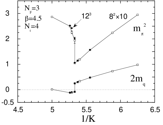
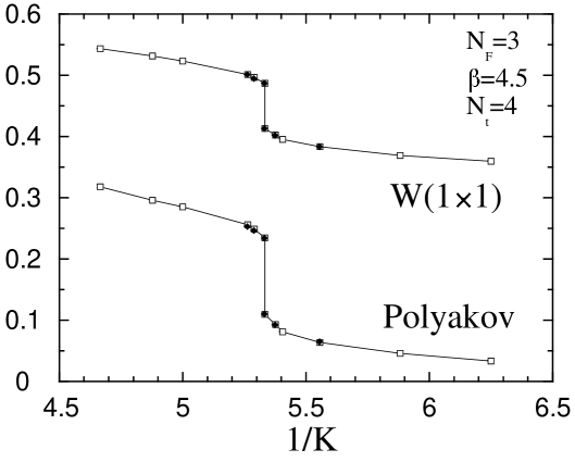
Figure 14: The same as Fig. 13 at $\beta=4.5$. The finite temperature transition $K_{t}$ locates at $K\simeq 0.1875$ ($1/K\simeq 5.33$).

Figure 15: The same as Fig. 13 at $\beta=4.7$ obtained on a $12^{3}\times 4$ lattice. The finite temperature transition $K_{t}$ locates at $K\simeq 0.1795$ ($1/K\simeq 5.57$).

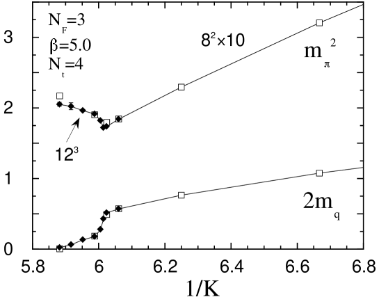
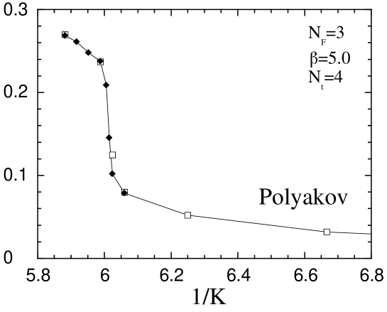
Figure 16: The same as Fig. 13 at $\beta=5.0$: (a) $m_{\pi}^{2}a^{2}$ and $2m_{q}a$, (b) the Polyakov loop. The finite temperature crossover $K_{t}$ locates at $K\simeq 0.166$ — 0.1665 ($1/K\simeq 6.01$ — 6.02).

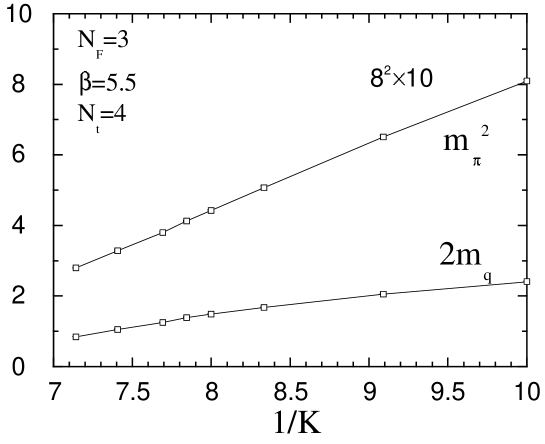
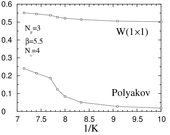
Figure 17: The same as Fig. 13 at $\beta=5.5$ obtained on an $8^{2}\times 10\times 4$ lattice. The finite temperature crossover $K_{t}$ locates at $K\simeq 0.125$ — 0.130 ($1/K\simeq 7.7$ — 8.0).

Figure 20: Time history of (a) $N_{\rm inv}$ and (b) the plaquette for $m_{s}\sim 150$ MeV on an $8^{2}\times 10\times 4$ lattice.

Figure 21: Time history of the plaquette for $m_{s}\sim 400$ MeV on a $12^{3}\times 4$ lattice.

References

- [1] R. Pisarski and F. Wilczek, Phys. Rev. D29 (1984) 338.
- [2] F. Wilczek, Int. J. Mod. Phys. A7 (1992) 3911; K. Rajagopal and F. Wilczek, Nucl. Phys. B399 (1993) 395.
- [3] Y. Iwasaki, K. Kanaya, S. Sakai and T. Yoshié, Nucl. Phys. B (Proc. Suppl.) 30 (1993) 327; ibid. 34 (1994) 314.
- [4] Y. Iwasaki, K. Kanaya, S. Sakai and T. Yoshié, preprint of Tsukuba UTHEP-300, to be published in Z. Phys. C71 (1996).
- [5] Y. Iwasaki, K. Kanaya, S. Kaya, S. Sakai and T. Yoshié, preprint of Tsukuba UTHEP-304, to be published in Z. Phys. C71 (1996); Nucl. Phys. B (Proc. Suppl.) 42 (1995) 499; K. Kanaya, Prog. Theor. Phys. Suppl. 120 (1995) 25.
- [6] K.G. Wilson, in New Phenomena in Subnuclear Physics, ed. A. Zichichi (Plenum, New York, 1977).
- [7] Y. Iwasaki, Nucl. Phys. B (Proc. Suppl.) 42 (1995) 96.
- [8] K. Kanaya, Nucl. Phys. B (Proc. Suppl.) 47 (1996) 144.
- [9] M. Bochicchio, L. Maiani, G. Martinelli, G. Rossi and M. Testa, Nucl. Phys. B262 (1985) 331.
- [10] S. Itoh, Y. Iwasaki, Y. Oyanagi and T. Yoshié, Nucl. Phys. B274 (1986) 33.
- [11] L. Maiani and G. Martinelli, Phys. Lett. 178B (1986) 265.
- [12] Y. Iwasaki, K. Kanaya, S. Sakai and T. Yoshié, Phys. Rev. Lett. 69 (1992) 21.
- [13] Y. Iwasaki, K. Kanaya, S. Sakai and T. Yoshié, Phys. Rev. Lett. 67 (1991) 1494.
- [14] Y. Iwasaki, T. Tsuboi and T. Yoshié, Phys. Lett. B220 (1989) 602.
- [15] D. Daniel, R. Gupta, G.W. Kilcup, A. Patel and S.R. Sharpe, Phys. Rev. D46 (1992) 3130.
- [16] C. Bernard et al., Phys. Rev. D49 (1994) 3574.
- [17] S. Aoki, Phys. Rev. D30 (1984) 2653; Phys. Rev. Lett. 57 (1986) 3136; Nucl. Phys. B314 (1989) 79; in the proceedings of the Japan-German Seminar QCD on Massively Parallel Computers (eds. A. Nakamura, K. Kanaya, and F. Karsch) [Prog. Theor. Phys. Suppl. 122 (1996)].
- [18] M. Fukugita, S. Ohta and A. Ukawa, Phys. Rev. Lett. 57 (1986) 1974.
- [19] S. Aoki, A. Ukawa, and T. Umemura, Phys. Rev. Lett. 76 (1996) 873; Nucl. Phys. B (Proc. Suppl.) 47 (1996) 511.
- [20] S. Duane, A.D. Kennedy, B.J. Pendleton and D. Roweth, Phys. Lett. B195 (1987) 216.
- [21] S. Gottlieb, W. Liu, D. Toussaint, R.L. Renken and R.L. Sugar, Phys. Rev. D35 (1987) 2531.
- [22] T. Blum, L. Kärkkäinen, D. Toussaint, and S. Gottlieb, Phys. Rev. D51 (1995) 5153.
- [23] F.R. Brown et al., Phys. Rev. D46 (1992) 5655.
- [24] Y. Oyanagi, Computer Phys. Commun. 42 (1986) 333; S. Itoh, Y. Iwasaki, Y. Oyanagi and T. Yoshié, Nucl. Phys. B274 (1986) 33.
- [25] M. Fukugita, Y. Oyanagi and A. Ukawa, Phys. Lett. B203 (1988) 145.
- [26] A. Ukawa, Nucl. Phys. B (Proc. Suppl.) 9 (1989) 463.
- [27] R. Gupta et al., Phys. Rev. D44 (1991) 3272.
- [28] K.M. Bitar et al., Phys. Rev. D49 (1994) 3546.
- [29] C. Bernard et al., ibid. D46 (1992) 4741; Nucl. Phys. B (Proc. Suppl.) 34 (1994) 324; T. Blum et al., Phys. Rev. D50 (1994) 3377.
- [30] R. Gupta et al., Phys. Rev. D40 (1989) 2072.
- [31] K. Bitar et al., Phys. Lett. B234 (1990) 333; Phys. Rev. D43 (1991) 2396.
- [32] Y. Iwasaki, K. Kanaya, S. Sakai and T. Yoshié, Nucl. Phys. B (Proc.Suppl.) 42 (1995) 502; Y. Iwasaki, K. Kanaya, S. Kaya, S. Sakai and T. Yoshié, Nucl. Phys. B (Proc. Suppl.) 47 (1996) 515; paper in preparation.
- [33] R. Gupta, G. Guralnik, G. Kilcup, A. Patel and S. Sharpe Phys. Rev. Lett. 57 (1986) 2621.
- [34] S. Itoh, Y. Iwasaki and T. Yoshié, Phys. Rev. D36 (1986) 527.
- [35] A. Ukawa, Lecture note for Ueling Summer School “Phenomenology and Lattice QCD”, Univ. of Washington, 1993 [Tsukuba preprint UTHEP-302 (1995)].
- [36] H. Meyer-Ortmanns, H.-J. Pirne, and A. Patkós, Phys. Lett. B295 (1992) 255; Int. J. Mod. Phys. C3 (1992) 993; S. Gavin, A. Gocksch and R.D. Pisarski, Phys. Rev. D49 (1994) R3079; D. Metzger, H. Meyer-Ortmanns and H.-J. Pirner, Phys. Lett. B321 (1994) 66; Erratum ibid. B328 (1994) 547.
- [37] H. Meyer-Ortmanns and B.-J. Schaefer, Phys. Rev. D53 (1996) 6586.
- [38] R.V. Gavai and F. Karsch, Nucl. Phys. B261(1985) 273; R.V. Gavai, J. Potvin and S. Sanielevici, Phys. Rev. Lett. 58(1987) 2519.
- [39] F.R. Brown et al., Phys. Rev. Lett. 65(1990) 2491.
- [40] For a review, A. Ukawa, Nucl. Phys. B (Proc. Suppl.) 30(1993) 3.
- [41] K.D. Born et al., Phys. Rev. D40(1989) 1653.
- [42] K. Rajagopal, in Quark-Gluon Plasma 2, ed. R. Hwa, World Scientific, 1995.
- [43] J.B. Kogut, D.K. Sinclair and K.C. Wang, Phys. Lett. B263 (1991) 101.
- [44] For recent reviews, K. Kanaya, Ref.[8]; C. DeTar, Nucl. Phys. B (Proc. Suppl.) 42 (1995) 73; F. Karsch, ibid. 34 (1994) 63.