Phase transition in fluctuating branched geometry

Abstract

We study grand–canonical and canonical properties of the model of branched polymers proposed in [1]. We show that the model has a fourth order phase transition and calculate critical exponents. At the transition the exponent $\gamma$ of the grand-canonical ensemble, analogous to the string susceptibility exponent of surface models, $\gamma\sim 0.3237525...$ is the first known example of positive $\gamma$ which is not of the form $1/n,\,n=2,3,\ldots$. We show that a slight modification of the model produces a continuos spectrum of $\gamma$’s in the range $(0,1/2]$ and changes the order of the transition.

,

Introduction

The problem of summing over random geometry appears in many areas of modern physics such as string theory, quantum gravity, membranes and others. The problem is known for being hard to study both analytically and numerically. Therefore one frequently uses simplified models. In many cases branched polymers capture some essential futures of more complicated models. Being simple and solvable they offer us insight into such issues like value of the string susceptibility exponent, correlation functions, renormalization group, sum over genera etc [1, 2, 3, 4].

In the present paper we study a model with a coupling to the branching of the polymers [1]. The model has two regimes. For small values of the coupling the exponent $\gamma=1/2$ while for larger values it is negative and depends linearly on the coupling. We extend the analysis from the original paper [1], localize the transition and find that at this point $\gamma\sim 0.3237525...$.

We also study the canonical ensemble and show that the model exhibits a fourth order phase transition. A slight modification of the model allowed us to obtain a continuos spectrum of $\gamma$’s between $0$ and $1/2$. In the canonical ensemble this generalized model can exhibit a phase transition of an arbitrary order equal or higher than 2.

The model

We consider an ensemble of planar rooted trees generated by the recursion relation shown in Fig.1.

Figure 1: Partition function

Each bubble in the figure denotes the grand canonical partition function $Z$. By iterating the relation one produces all possible planar rooted trees. Each tree contributes to the partition function the factor $e^{-\mu n}$, where $n$ is the number of vertices in the tree. Each vertex additionally contributes a weight factor depending on its degree, ie the number of branches which meet at vertex. In Fig.1 we denoted these weight factors by $t_{k}$, where $k$ is degree of vertex. In this paper we analyze the model with $t_{k}=k^{-\beta}$, where $\beta$ is an external parameter. The equation from Fig. 1 can be written as :

$$Z(\mu,\beta)=e^{-\mu}\sum_{k=1}^{\infty}\frac{Z(\mu,\beta)^{k-1}}{k^{\beta}}$$ (1)

which generates following partition function (in the following we drop the arguments of the $Z$ function)

$$Z=\sum_{T\in{\mathcal{T}}}e^{-\mu n(T)}e^{-\beta E(T)}$$ (2)

where $\mathcal{T}$ denotes the ensemble of all trees. The function $E(T)$ plays the role of energy which the tree contributes to the ensemble and is equal :

$$E(T)=\sum_{v\in T}\ln k(v)$$ (3)

The sum goes over all vertices of the tree $T$, and $k(v)$ is degree of vertex $v$. By summing first over trees with fixed number of vertices we rewrite (2) as

$$Z=e^{-\phi}=\sum_{n=1}^{\infty}z_{n}e^{-\mu n}=\sum_{n=1}^{\infty}e^{n(f_{n}-\mu)}$$ (4)

The coefficients $z_{n}$ of the series at $e^{-\mu n}$ depend on $\beta$ and correspond to a sum of $e^{-\beta E(T)}$ over the ensemble of all trees with $n$ vertices. They are canonical partition functions for the ensembles of trees with $n$ nodes. We have introduced convenient variables which we will use later on : free energy density $f_{n}(\beta)$ for the system with $n$ vertices defined from the expansion coefficients : $z_{n}=e^{nf_{n}}$ and thermodynamic potential which we call free enthalpy $\phi=-\ln Z$.

For large positive $\beta$ the canonical partition function is dominated by branched polymers with minimal energy. Such branched polymers maximize the number of vertices in the last generation ie vertices with degree $k=1$. They look like short bushes. In the extreme case such bushes have one branched vertex with $n$ branches while all other vertices belong to the last generation. The energy of such branched polymers is $\ln n$. When $\beta$ becomes smaller the entropy becomes important and more and more elongated structures appear in the ensemble. At certain $\beta$ the system undergoes a fourth order phase transition associated with the change of the regimes. Finally if one allowed for negative $\beta$ then for large negative $\beta$, trees with large energy would mainly contribute to the canonical ensemble. The maximal energy $E$ for the system with $n$ nodes is $n\ln 2$ and comes from the chain structure.

Exponent $\gamma$

The series (4) representing the grand canonical partition function $Z$ is regular at $e^{-\mu}=0$. The behaviour of $z_{n}$ in the thermodynamic limit $n\rightarrow\infty$ can be deduced from the behaviour of the function $Z$ at the radius of convergence $e^{-\mu_{0}}$, when $\mu\rightarrow\mu_{0}^{+}$, which corresponds to the first singularity of $Z$ encountered when $\mu$ comes from $\infty$. At this singularity free enthalpy as a function of chemical potential behaves for a given $\beta$ as :

$$\phi-\phi_{0}\sim(\mu-\mu_{0})^{1-\gamma}$$ (5)

where $\phi_{0}$, $\mu_{0}$ and $\gamma$ depend on $\beta$. The parameter $\mu_{0}$ is the critical value of the chemical potential and $\gamma$ is the universal exponent defining a type of singularity which accounts for the universality class a model belongs to. Its counterpart in the surface models is called the string susceptibility exponent. As will be seen later $\gamma$ is equal or less than $1/2$ and therefore the function on the right hand side goes to $0$ when $\mu$ approaches $\mu_{0}$. The value of free enthalpy at $\mu=\mu_{0}$ is denoted by $\phi_{0}=\phi(\mu_{0})$. The singularity $(\ref{phis})$ corresponds to the following asymptotic behaviour of the coefficients $z_{n}$ in the limit of large $n$ :

$$z_{n}(\beta)\sim n^{\gamma-2}e^{n\mu_{0}}$$ (6)

In the thermodynamic limit $n\rightarrow\infty$ the free energy density is $f_{\infty}(\beta)=\mu_{0}(\beta)$.

The series $Z(\mu)$ is given by an indirect relation (1) which can be rewritten

$$\mu(\phi,\beta)=\ln L_{\beta}(e^{-\phi})+2\phi$$ (7)

where $L_{\beta}(z)=\sum_{n=1}^{\infty}z^{n}/n^{\beta}$ is a special function whose basic properties, frequently used in this paper, are listed in the appendix. Throughout the paper we use convention for functions which have $\beta$ as second argument that prime denotes derivative at fixed $\beta$. The function $\phi(\mu)$ is singular at $\mu_{0}$ when either $\mu^{\prime}(\phi_{0})=0$ or $\mu(\phi_{0})$ itself is singular at $\phi_{0}=\phi(\mu_{0})$. The first condition reads

$$\mu^{\prime}(\phi_{0},\beta)=\frac{\partial\mu(\phi_{0},\beta)}{\partial\phi}=0$$ (8)

which, by virtue of (39), simplifies to :

$$2L_{\beta}(e^{-\phi_{0}})=L_{\beta-1}(e^{-\phi_{0}})$$ (9)

The solution of (9) is shown in Fig. 2.

Figure 2: Critical free enthalpy

The function $\phi_{0}$ approaches its critical value $\phi_{C}=0$ when $\beta\rightarrow\beta_{C}$. At this point the argument of $L_{\beta}$ : $e^{-\phi_{0}}$ becomes unity and is equal to the radius of convergence of $L_{\beta}$. For $\beta>\beta_{C}$ the critical value of $\phi$ stays at $\phi_{C}=0$ and corresponds directly to the singularity of the map $\mu(\phi,\beta)$ . Inserting $e^{-\phi_{0}}=1$ to the (9) we get the critical value of $\beta$ :

$$2\zeta(\beta_{C})=\zeta(\beta_{C}-1)$$ (10)

which can be found numerically $\beta_{C}=2.4787508...$.

Inserting this back into $\mu$ we get the critical value of the chemical potential at the radius of convergence of the series (4) which also corresponds to the free energy density in the thermodynamic limit $f_{\infty}(\beta)$ :

$$f_{\infty}(\beta)=\mu_{0}=\mu(\phi_{0}(\beta),\beta)=\left\{\begin{array}[]{lr}\ln L_{\beta}(e^{-\phi_{0}(\beta)})+2\phi_{0}(\beta),&\quad\beta<\beta_{C}\\ \ln L_{\beta}(1)=\ln\zeta(\beta),&\quad\beta\geq\beta_{C}\end{array}\right.$$ (13)

We can now compute the exponent $\gamma$. We separately consider three cases
$\beta<\beta_{C}$, $\beta=\beta_{C}$ and $\beta>\beta_{C}$. We invert the function $\mu(\phi)$ (7) with respect to $\phi$, for $\phi$ near to $\phi_{0}$. For $\beta<\beta_{C}$ we have :

$$\mu-\mu_{0}=\frac{\mu_{0}^{\prime\prime}}{2}(\phi-\phi_{0})^{2}+\dots$$ (14)

and from there

$$(\phi-\phi_{0})=\bigg{(}\frac{2}{\mu_{0}^{\prime\prime}}\bigg{)}^{1/2}(\mu-\mu_{0})^{1/2}+\dots$$ (15)

The second derivative $\mu_{0}^{\prime\prime}$ is finite in this range. For $\beta=\beta_{C}$ the expansion starts directly from the singular term :

$$\mu-\mu_{0}=w(\beta_{C})(\phi)^{\beta_{C}-1}+\dots$$ (16)

because $\mu^{\prime}=0$ at this point and $\beta_{C}$ is between $2$ and $3$. The coefficient $w(\beta)=\Gamma(1-\beta)/\zeta(\beta)$. Inverting this with respect to $\phi$ we obtain :

$$\phi=w(\beta_{C})^{1/(\beta_{C}-1)}(\mu-\mu_{0})^{1/(\beta_{C}-1)}+\dots$$ (17)

Finally, for $\beta>\beta_{C}$ the expansion of $\mu$ around $\mu_{0}$ starts with a nonvanishing linear part :

$$\mu-\mu_{0}=\mu_{0}^{\prime}\phi+\dots+w(\beta)\phi^{\beta-1}+\dots$$ (18)

The dots between the terms $\phi$ and $\phi^{\beta-1}$ correspond to integer powers $\phi^{n}$ with $n$ less than $\beta$ (see (41)). Inverted with respect to $\phi$ the equation yields :

$$\phi=\frac{1}{\mu_{0}^{\prime}}(\mu-\mu_{0})+\dots-\frac{w(\beta)}{(\mu_{0}^{\prime})^{\beta}}(\mu-\mu_{0})^{\beta-1}+\dots$$ (19)

Comparing the singularities with (5) we obtain :

$$\gamma=\left\{\begin{array}[]{lr}\displaystyle\frac{1}{2},&\quad\beta<\beta_{C}\\ \frac{\displaystyle\beta_{C}-2}{\displaystyle\beta_{C}-1}=0.3237525...,&\quad\beta=\beta_{C}\\ 2-\beta,&\quad\beta>\beta_{C}\end{array}\right.$$ (23)

Canonical ensemble

Properties of the canonical ensemble in the thermodynamic limit are described by the free energy density $f_{\infty}(\beta)$. It is a continuos function of $\beta$ but it has singularity at $\beta=\beta_{C}$. To extract the dominating singularity of free energy for $\Delta\beta=(\beta_{C}-\beta)\rightarrow 0^{+}$ let us first consider the critical free enthalpy $\phi_{0}(\beta)$ defined by the equation (9). Using (41) we can for small $\beta$ and $\phi_{0}$ expand the equation (9) :

$$-a\Delta\beta+b\phi_{0}^{\beta_{C}-2}+...=0$$ (24)

up to $o(\Delta\beta)$ and $o(\phi_{0}^{\beta_{C}-2})$ . The expansion coefficients are $a=2\zeta^{\prime}(\beta_{C})-\zeta^{\prime}(\beta_{C}-1)=3.4950...$, $b=-\Gamma(2-\beta_{C})=3.5548...$. Solved for $\phi_{0}$ the last equation gives

$$\phi_{0}(\beta)=c\Delta\beta^{3-\eta}+...$$ (25)

in the limit $\Delta\beta\rightarrow 0^{+}$. The exponent $\eta=3-1/(\beta_{C}-2)=0.911231...$, and the coefficient $c=(a/b)^{1/(3-\eta)}=0.9666...$. We can now insert $\phi_{0}$ into (13) and compute singularity of $f_{\infty}(\beta)$. The first derivative is :

$$f_{\infty}^{\prime}(\beta)=\frac{\partial\mu(\phi_{0},\beta)}{\partial\phi}\phi_{0}^{\prime}+\frac{\partial\mu(\phi_{0},\beta)}{\partial\beta}=\frac{(\partial_{\beta}L_{\beta})(e^{-\phi_{0}})}{L_{\beta}(e^{-\phi_{0}})}$$ (26)

The term containing $\partial\mu/\partial\phi$ vanishes identically for $\phi_{0}$ (8). Now we can expand the last expression in small $\phi_{0}$, and then in small $\Delta\beta$. The dominating singularity for $\Delta\beta\rightarrow 0^{+}$ comes from the first nonvanishing term containing $\phi_{0}$. This term is linear in $\phi_{0}$ and introduces the singularity $\Delta\beta^{3-\eta}$ :

$$f_{\infty}^{\prime}(\beta)=\frac{\zeta^{\prime}(\beta)}{\zeta(\beta)}+d\Delta\beta^{3-\eta}+...$$ (27)

The coefficient in front of the singular term :

$$d=c\frac{\zeta^{\prime}(\beta_{C})}{\zeta(\beta_{C})}\Bigg{(}\frac{\zeta(\beta_{C}-1)}{\zeta(\beta_{C})}-\frac{\zeta^{\prime}(\beta_{C}-1)}{\zeta^{\prime}(\beta_{C})}\Bigg{)}=2.4990...$$

is obtained by expanding (26) and using (41). The first term on the right hand side of (27) matches the function for $\beta>\beta_{C}$ (13) and solutions come smoothly one into the other. The contribution of the singular term $(\Delta\beta)^{3-\eta}$ vanishes at $\Delta\beta=0$ as well as for the second and the third derivative of the free energy density $f_{\infty}$. For the fourth derivative the singular term blows up at $\beta_{C}$ :

$$\frac{d^{4}f_{\infty}}{d\beta^{4}}(\beta_{C}^{-})-\frac{d^{4}f_{\infty}}{d\beta^{4}}(\beta_{C}^{+})=e\Delta\beta^{-\eta}+...$$ (28)

where $e=(3-\eta)(2-\eta)(1-\eta)d=0.5045...$. This shows that the model has a fourth order phase at $\beta_{C}$ in the canonical sector with a singularity given by the exponent $\eta$.

Non–universality

The dependence of the exponent $\gamma$ on the critical value of the coupling suggests a non–universality. By changing slightly the model one should be able to change the value of $\beta_{C}$ without spoiling the formulas (23). In this way one can change the value of the exponent $\gamma_{C}$. We will show below that indeed a simple modification of the model produces a whole continuos spectrum of $\gamma$’s.

We modify the model by letting the weight $t_{1}$, coupled to the number of points of the last generations, vary in contrast to the model defined by (1) where it was set to $1$. Now $t_{1}$ can take arbitrary value greater than zero. The value of $t_{1}$ affects the number of points in the last generation. Decreasing/increasing $t_{1}$ for a given $\beta$ favours/suppresses polymers with many points in the last generation. By changing $t_{1}$ we can shift the critical value of $\beta$ where the phase transition takes place. On the other hand this modification does not change the singularity of the function on right hand–side of (1).

After introducing the modification of the weight $t_{1}$ the equation (7) becomes :

$$\mu(\phi,\beta)=\ln\{L_{\beta}(e^{-\phi})+(t_{1}-1)\e^{-\phi}\}+2\phi$$ (29)

Repeating the analysis from the previous sections we first find the critical line $\phi_{0}$ as a solution of $\mu^{\prime}=0$ :

$$L_{\beta}(e^{-\phi})-L_{\beta-1}(e^{-\phi})=(1-t_{1})e^{-\phi}$$ (30)

for $\beta$ less than $\beta_{C}$ and $0$ for $\beta$ greater than $\beta_{C}$. The position of the critical point is given by :

$$2\zeta(\beta_{C})-\zeta(\beta_{C}-1)=1-t_{1}$$ (31)

The value $\beta_{C}$ as a function of $t_{1}$ is shown in Fig.3. For $t_{1}\rightarrow+\infty$, the value of $\beta_{C}$ goes to $2$. For $t_{1}\rightarrow 0$, $\beta_{C}$ goes to infinity.

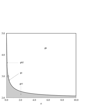
Figure 3: Phase diagram of the extended model

As first, consider the case $2<\beta_{C}<3$ corresponding to $t>t^{*}_{1}=1+\zeta(2)-2\zeta(3)=0.24081\ldots$ . Repeating the same analysis as for the original model we get that $\gamma$ is given exactly by the same formula (23) with $\beta_{C}$ replaced now by the current value $\beta_{C}(t_{1})$. At the critical point we have $\gamma_{C}=(\beta_{C}-2)/(\beta_{C}-1)$ which changes contiuosly between $0$, $1/2$ when $\beta_{C}$ goes from $2$ to $3$. When $\beta_{C}$ exceeds $3$, which is for $t_{1}<t^{*}_{1}$, the situation changes. The expansion (16) starts then not from the singular term with the power $\beta_{C}-1$ but from the term $\mu^{\prime\prime}_{0}\phi^{2}$ which after inverting gives the singularity $\phi\sim(\mu-\mu_{0})^{1/2}$ and hence $\gamma=1/2$.

To find the type of the singularity in the canonical ensemble we determine the behaviour of the critical free enthalpy for $\Delta\beta=(\beta-\beta_{C})\rightarrow 0^{+}$ . As before first consider the case $2<\beta_{C}<3$. Expanding the equation $\mu^{\prime}=0$ for small $\Delta\beta$ and small $\phi$ we get exactly the same equation as (24) with exactly the same coefficients but calculated now at different $\beta_{C}$. The function $\phi_{0}$ has then the singularity $\phi_{0}\sim(\Delta\beta)^{1/(\beta_{C}-2)}$ whose power depends through $\beta_{C}$ on the parameter $t_{1}$ and varies continuosly.

The situation changes for $\beta_{C}>3$ ($t_{1}<t^{*}_{1}$) because then additionally regular terms in $\phi_{0}$ enter the expansion. They introduce powers of $\phi_{0}$ smaller than $\phi_{0}^{\beta_{C}-2}$ :

$$-a\Delta\beta+g\phi_{0}+\dots+b\phi_{0}^{\beta_{C}-2}+...=0$$ (32)

where $g=-2\zeta(\beta_{C}-1)+\zeta(\beta_{C}-2)$, and $a,b$ are as in the equation (24). Inverting the last equation for $\phi_{0}$ as a function of $\Delta\beta$ we get :

$$\phi_{0}=\frac{a}{g}\Delta\beta+\dots-\frac{b}{g}\big{(}\frac{a}{g}\big{)}^{(\beta_{C}-2)}\Delta\beta^{(\beta_{C}-2)}\dots$$ (33)

Inserting the singularity of $\phi_{0}$ into $f^{\prime}_{\infty}$ analogously as we did in (27) we obtain the singular part of the first derivative of the free energy :

$$f^{\prime}_{\infty}\sim\left\{\begin{array}[]{lr}\Delta\beta^{1/(\beta_{C}-2)},&\quad t_{1}>t^{*}_{1}\\ \Delta\beta^{\beta_{C}-2},&\quad t_{1}<t^{*}_{1}\end{array}\right.$$ (36)

One sees that the order of the transition grows arbitraryly and the transitions gets softer when $\beta_{C}$ approaches $2$, corresponding to $t_{1}\rightarrow 0$, or when $\beta_{C}$, $t_{1}\rightarrow\infty$. The strongest transition takes place for $t_{1}=t^{*}_{1}$ for which $\beta_{C}=3$ and the second derivative of the free energy diverges logarithmically $\ln(\Delta\beta)$.

Discussion

The model described above exhibits a manifold behaviour summarized on the phase diagram $(t_{1},\beta)$ (Fig.3). The model has two phases with bush and tree like branched polymers. They are separated by a critical line on which the order of the transition and the critical exponents vary. It has a stable phase for $\beta<\beta_{c}(t_{1})$ where the exponent $\gamma=1/2$ and it is not affected by a perturbation of couplings. This is a generic branched polymer phase and has realizations in surface models and higher simplicial gravity [5]. At the critical line $\beta_{C}(t_{1})$ the exponent $\gamma$ is unstable against small changes of the model parameters and reveals a continuos spectrum in the interval $(0,1/2]$.

It is known that for $c>1$ exponent $\gamma$ is not universal which means that $\gamma$ depends not only on $c$ but also on additional parameters controlling a specific model realization. For example, for gaussian field on random surface the exponent $\gamma$ changes as a function on the number of fields $c$ and the integration measure parameter [6]. A classification for a certain subclass of models was listed by Durhuus [7] who showed that positive $\gamma$ is of the form $1/n$ $n=2,3,...$ and in particular $\gamma=1/3$ is realized by multispin models. Our results do not prove that surface models with arbitrary $\gamma$ in the range $(0,1/2]$ do exist but surely make it more plausible.

We believe that models of branched polymers are worth studying not only in the above mentioned context of universality of random surfaces but also as solvable models for fluctuating geometry. Our present understanding of critical phenomena is mainly based on the spin type models on regular fixed geometry. One wonders if this intuition can be translated directly to fluctuating geometry. In particular, there is a difficulty with defining correlation functions on fluctuating geometry since the distance between points fluctuates [3, 8]. A study of models as the one discussed here, especially around the phase transition, can hopefully give us a more profound understanding of those problems.

Appendix

We shortly summarize properties of the function defined by the series :

$$L_{\beta}(z)=\sum_{n=1}^{\infty}\frac{z^{n}}{n^{\beta}}$$ (37)

For $z=1$ and $\beta>1$ the function reduces to the Riemann Zeta function :

$$L_{\beta}(1)=\zeta(\beta)$$ (38)

Calculating derivative with respect to the argument $z$ we get within the radius of convergence $|z|<1$ :

$$z\frac{dL_{\beta}(z)}{dz}=L_{\beta-1}(z)$$ (39)

which also holds for $z=1$ when $\beta>2$. The function $L_{\beta}(z)$ has singularity when $z\rightarrow 1$ of the type :

$$\mbox{sing }L_{\beta}(z)\sim\Gamma(1-\beta)(1-z)^{\beta-1},\qquad\beta\neq 1,2,\ldots$$ (40)

where $\Gamma$ is the Euler gamma function.

Put together, the last equations give for $x\rightarrow 0$ :

$$L_{\beta}(1-x)=\zeta(\beta)+\dots+(-)^{n}\zeta(\beta-n)\frac{x^{n}}{n!}+\Gamma(1-\beta)x^{\beta-1}$$ (41)

up to $o(x^{\beta-1})$. $n$ is the largest integer less than $\beta-1$. For integer $\beta$’s the dominating singularity is of the type $x^{\beta-1}\ln x$.

References

- [1] J. Ambjørn, B. Durhuus, J. Fröhlich, P. Orland Nucl. Phys. B270 (1986) 457.
- [2] J. Ambjørn, B. Durhuus, Jónsson Phys.Lett. B244 (1990) 403-412.
- [3] P. Bialas, Phys. Lett. B373 (1996) 289.
- [4] J. Ambjørn, P. Bialas, J. Jurkiewicz, RG flow in an exactly solvable model with fluctuating geometry.,e-Print Archive: hep-lat/9602021
- [5] J. Ambjørn, J. Jurkiewicz, Nucl. Phys. B541 (1995) 643.
- [6] F. David, J. Jurkiewicz, A. Krzywicki, B. Petersson, Nucl. Phys. B290 (1987) 218.
- [7] B. Durhuus, Nucl.Phys. B426 (1994) 203.
- [8] Bas V. de Bakker, Jan Smit, Nucl.Phys.B454 (1995) 343