BUTP–96/13

SU(3) Thermodynamics on Small Lattices

Alessandro Papa

Institute for Theoretical Physics

University of Bern

Sidlerstrasse 5, CH–3012 Bern, Switzerland

March 2024

Abstract

The free energy density of the SU(3) gauge theory at temperatures $T/T_{c}=4/3,3/2$ and 2 is calculated on lattices with temporal extent as small as $N_{\tau}=2,3$ and spatial extent $N_{\sigma}=4N_{\tau}$ using parametrized fixed point actions. Although cut–off effects are seen, they are hugely suppressed with respect to Wilson and Symanzik–improved actions and at $N_{\tau}=3$ there is already a good agreement with the continuum limit as extrapolated from the results with the Wilson action at $N_{\tau}=6$ and 8.

PACS number(s): 05.70.Ce, 11.10.Wx, 11.10.Hi, 12.38.Gc, 12.38.Mh

1 Introduction

Understanding the high temperature phase of QCD is of great importance especially in astronomy and cosmology. In such a phase quarks and gluons are expected to behave like a plasma of weakly interacting particles approximately described by an ideal gas. To find signatures of this plasma is the central goal of present and forthcoming experiments in heavy–ion collisions at CERN and BNL.

Owing to the well–known infrared problem [1] of finite temperature QCD, the perturbative expansions of thermodynamic quantities can be calculated only up to $g^{5}$ order and their convergence is very bad even at temperatures much larger than $T_{c}$ [2, 3]. Lattice numerical simulations are therefore an essential tool in investigating QCD at high temperatures, where non–perturbative effects seem to be important at least in the vicinity of the phase transition.

In lattice numerical simulations, the temperature $T$ and the volume $V$ are determined by the lattice size $N_{\sigma}^{3}\times N_{\tau}$, $N_{\tau}<N_{\sigma}$ through

$$T\;=\;\frac{1}{N_{\tau}a}\;\;\;,\;\;\;\;\;\;V\;=\;(N_{\sigma}a)^{3}\;\;\;,$$ (1)

and (anti–)periodic boundary conditions have to be imposed in the time direction for (Fermi) Bose fields. The lattice spacing $a$ depends on the coupling $\beta=2N/g^{2}$; the asymptotic form of this dependence can be known analytically from perturbation theory.

At high temperatures, high momentum modes give relevant contributions to the free energy density. In this regime, thermodynamic quantities are therefore strongly influenced by the finite lattice cut–off $a^{-1}$ introduced by the discretization of the theory. This cut–off effect manifests itself in $O(a^{2})$ (i.e. $O(1/N_{\tau}^{2})$ at fixed $T$) corrections which vanish in the continuum limit. How large $N_{\tau}$ has to be in order to allow reliable extrapolations to the continuum depends on the specific regularization of the theory, i.e. on the lattice action.

The Wilson plaquette action [4] is the simplest action which can be used in numerical simulations of the pure gauge theory. It has however the disappointing drawback of introducing large cut–off dependences in physical observables: in zero temperature simulations, the continuum limit is reached at lattice spacings smaller than 0.1 fm, so physics at the hadronic scales can be simulated only on uncomfortably large lattices. One can have a feeling of the relevance of cut–off effects with the SU(N) Wilson action looking at the expressions for the energy density $\epsilon$ and the pressure $p$ of the gas of gluons in the $T\rightarrow\infty$ limit [5, 6]

$$\frac{\epsilon}{T^{4}}=\frac{3p}{T^{4}}=(N^{2}-1)\frac{\pi^{2}}{15}\left[1+\frac{30}{63}\left(\frac{\pi}{N_{\tau}}\right)^{2}+\frac{1}{3}\left(\frac{\pi}{N_{\tau}}\right)^{4}+O\left(\frac{1}{N_{\tau}^{6}}\right)\right]\;\;\;.$$ (2)

The deviation from the Stefan–Boltzmann law $(N^{2}-1)\pi^{2}/15$ is very prominent: for $N_{\tau}=4$, where also $O(1/N_{\tau}^{6})$ contributions are not negligible, the deviation from the continuum is about 50% [6]. The relevance of cut–off effects in SU(3) thermodynamic quantities at temperatures $T$ equal to a few times $T_{c}$ is less dramatic [7, 8], but large enough to call for lattices up to $32^{3}\times 8$ before safely extrapolating to the continuum. Since fluctuations in thermodynamic quantities go like $1/\sqrt{V_{4}}\sim N_{\tau}^{-2}$, a constant accuracy requires a computational effort which increases at least like $N_{\tau}^{10}$ (here, a fixed $N_{\sigma}/N_{\tau}$ ratio has been assumed).

Adopting the Symanzik program [9] to improve actions reduces indeed lattice artifacts. Since the improvement procedure is perturbative, the benefit is expected only at large values of the coupling $\beta$, i.e. at large temperatures $T$ for fixed $N_{\tau}$. Indeed, in SU(N) lattice gauge theory in the $T\rightarrow\infty$ limit, the first correction to the Stefan–Boltzmann law can be made $O(1/N_{\tau}^{4})$, if the action is improved at the tree level with a $1\times 2$ or a $2\times 2$ plaquette, or even $O(1/N_{\tau}^{6})$, if it is improved with a $2\times 2$ and a $3\times 3$ plaquette [6]. For $N_{\tau}=4$ the deviation from the Stefan–Boltzmann law is $1.34\%$ with the $1\times 2$ improvement and $8.77\%$ with the $2\times 2$ one [6].

As a radical solution of the problem of cut–off effects in lattice simulations, P. Hasenfratz and F. Niedermayer [10] have recently suggested to use perfect lattice actions, i.e. actions which are completely free of cut–off effects. The existence of such actions is well established in the Wilson’s renormalization group (RG) theory [11]. The fixed point (FP) action and the renormalized trajectory of a RG transformation define a perfect quantum action. For an asymptotically free theory, the FP action itself reproduces the properties of the continuum classical action – it is the perfect classical action. A formal argument of perturbative RG implies that FP actions are also 1–loop (quantum) perfect [12, 13]. FP actions are therefore the first step in the ambitious program of building perfect lattice actions.

In Ref. [10] a general method for the determination of FP actions for asymptotically free theories was proposed, which was successfully applied to the 2–d O(3) non–linear $\sigma$–model on the lattice. A parametrization of the FP action suitable for numerical simulations was found showing no cut–off effects up to correlation lengths as small as $\xi\sim 3$ lattice spacings, i.e. well away from the continuum limit. Moreover, a perturbative calculation [14] of the mass gap in a periodic box of size $L$, $m(L)$, using the lattice FP action showed that cut–off effects are absent also on the 1–loop level.

A similar program has been carried out for SU(3) lattice gauge theory [13, 15] starting from two different RG transformations (type I and type II in the following). A few–parameter approximation has also been suggested [15] for both type I and type II FP actions in terms of the plaquette and the twisted perimeter–six loop. Preliminary scaling tests of the type I FP action on the torelon mass and the static $q\bar{q}$ potential, using the critical deconfining temperature to set the scale, have already shown a clear improvement with respect to the Wilson action [15].

The aim of this paper is to perform a study of the cut–off effects of parametrized FP actions in bulk thermodynamic quantities of the SU(3) gauge theory at finite temperature. Indeed, the contribution of high excitations to these quantities is important, making lattice determinations quite sensitive to the cut–off. FP actions are implemented on lattices as small as $8^{3}\times 2$ and $12^{3}\times 3$ to calculate the free energy density at temperatures $T/T_{c}=4/3,\ 3/2,\ 2$.

The paper is organized as follows:
in Section 2 the construction of a (parametrized) FP action is shortly recalled and some comments are presented about the expected cut–off effects in the free energy density;
in Section 3 elements and techniques of lattice finite temperature SU(3) thermodynamics relevant to the remaining part of the paper are briefly reviewed;
in Section 4 Monte Carlo (MC) determinations of the free energy density with parametrized FP actions are compared with previous results with Wilson and Symanzik–improved actions.

2 Parametrized FP actions and cut–off effects in the free energy density

The partition function of an SU(N) gauge theory defined on a hypercubic lattice is

$$Z=\int DU\>e^{-\beta A(U)}\;\;\;,$$ (3)

where $\beta A(U)$ is some lattice regularization of the continuum action expressed in terms of products of link variables $U_{\mu}(n)=e^{iA_{\mu}(n)}\in$SU(N) along arbitrary closed loops. If $\beta$, $c_{2},c_{3},\ldots$ denote the couplings of $\beta A(U)$, the action can be represented by a point in the infinite dimensional space of the couplings (see Fig. 1).

Figure 1: Schematic flow diagram for asymptotically free gauge theories.

Under repeated RG transformations the action moves in the space of couplings. A RG transformation with scale factor 2 can be defined in the following way:

$$e^{-\beta^{\prime}A^{\prime}(V)}=\int DU\>e^{-\beta(A(U)+T(U,V))}\;\;\;;$$ (4)

here $V$ is the coarse link living on the lattice with spacing $a^{\prime}=2\,a$, related to a local average of the original link variables $U$; $T(U,V)$ is the blocking kernel which defines this average, normalized in order to keep the partition function (and therefore the free energy) invariant under the transformation. There is a wide freedom in defining the RG average; this freedom can be exploited for optimization in numerical simulations.

On the critical surface $\beta=\infty$, Eq. (4) leads to the saddle point equation:

$$A^{\prime}(V)=\min_{\{U\}}[\,A(U)+T(U,V)\,]\;\;\;;$$ (5)

the FP point of this transformation is therefore

$$A^{FP}(V)=\min_{\{U\}}[\,A^{FP}(U)+T(U,V)\,]\;\;\;.$$ (6)

An important consequence of this equation is that if the configuration $\{V\}$ satisfies the FP classical equations and is a local minimum of $A^{FP}(V)$ then the fine configuration $\{U(V)\}$ minimizing the r.h.s. of Eq. (6) satisfies the FP classical equations as well and the value of the action remains unchanged, $A^{FP}(V)=A^{FP}(U(V))~{}$[10, 13]. As a consequence, the FP action has exact scale invariant instanton solutions with the same action as in the continuum theory.

Although the FP lies on the critical surface $\beta=\infty$, by the expression “FP action” we mean $\beta A^{FP}(U)$ which corresponds to the line which leaves orthogonally the critical surface, i.e. $\beta A^{FP}(U)\rightarrow\beta^{\prime}[A^{FP}(U)+O(1/\beta^{2})]$. For very large $\beta$, the FP action stays close to the RT, i.e. it is a good approximation of the perfect action. This follows from a formal argument [12, 13] of perturbative RG implying that FP actions are perfect not only in the classical limit $\beta=\infty$, but also at 1–loop order of perturbation theory. The range of $\beta$ for which the FP action and the RT stay close together cannot be known a priori just by looking at the RG transformation.

The FP equation (6) is highly non–trivial. On smooth $V$ configurations, it can be expanded in powers of the vectors potential and studied analytically. At the lowest order in the expansion of the vector fields the FP action is quadratic and can be found analytically [13]: it describes massless free gluons with an exact relativistic spectrum for all values of the momenta, i.e. not restricted to the first Brillouin zone.

On configurations with large fluctuations, numerical methods have to be used to solve Eq. (6). For practical reasons, however, it is useful to find a general parametrization for the FP action, simple enough to be used in Monte Carlo simulations. In Ref. [13] two RG transformations (type I and type II) were defined depending both on two parameters which were optimized in order to make the quadratic part of the FP action the most short ranged. The type I FP action (which is used in the following) was parametrized with powers of the real part of the trace of the plaquette and the twisted perimeter–six loop, calling for (only) 8 parameters.

The source of cut–off effects in determinations of the free energy density on the lattice using parametrized FP actions as regularization is three–fold:

i. Although the blocking kernel $T(U,V)$ is normalized in order to keep the partition function invariant under the RG transformation, a field–independent term in $A^{\prime}(V)$ appears in Eq. (4) as a result of integration on the fine links $U$. The amount of this constant term can be singled out plugging the flat configuration of the coarse lattice ($V_{\mu}(n_{B})=1$ for every site $n_{B}$) into Eq. (4): it is easy to see that it is given by the sum of quantum fluctuations around the flat configuration of the fine lattice. One usually discards this term since it does not affect the dynamics of the coarse field. For $N_{\tau},N_{\sigma}$ (a few times) larger than the “size of the action” this term is proportional to the lattice volume $N_{\sigma}^{3}N_{\tau}$ and gives again a constant (independent of $N_{\tau}$ and $N_{\sigma}$) contribution to the free energy density which can be discarded as well. However, for very small $N_{\tau}$ (and/or $N_{\sigma}$) the field–independent part will depend non–trivially on $N_{\tau}$. This produces an artifact which decreases exponentially with $N_{\tau}$. In practice, it will show up only for $N_{\tau}=2$.
It should be stressed that all the above observations hold even in the classical limit.

ii. The perfect action at finite $\beta$ is represented by the points on the RT. At moderate values of $\beta$, the FP action deviates from the RT: this deviation causes cut–off effects.

iii. The parametrization of a FP action introduces additional cut–off effects. This is especially true for the few–coupling parametrizations needed to perform numerical simulations. In most cases parametrizations are reliable only in the region of correlation lengths in which the numerical procedure to fix the parameters was performed.

While cut–off effects referred in ii. are not fully under control, those referred in iii. can be considerably reduced if a “good” parametrization is found. Short range actions are easier to parametrize than extended actions. Experience with RG suggests that a good averaging procedure in the block transformation will decrease the extension of the corresponding FP action. In Ref. [16] a new RG transformation has been proposed with a smoother and more rotational symmetric smearing kernel $T(U,V)$, with a larger number of free parameters used to optimize the resulting FP action. Preliminary scaling test of this type III FP action with the static $q\bar{q}$ potential have already shown an improvement of the performances with respect to the type I FP action (using the same 8–coupling parametrization) [16].

3 SU(3) thermodynamics on the lattice

All the continuum thermodynamic quantities for a system with zero chemical potential can be derived from the free energy density

$$f\;=\;-\frac{T}{V}\ln Z(T,V)\;\;\;,$$ (7)

where $V$ is the volume of the system, $T$ the temperature and $Z$ the canonical partition function. The energy density $\epsilon$ and the pressure $p$ are determined by the formulae

$$\epsilon = \frac{T^{2}}{V}\frac{\partial\ln Z(T,V)}{\partial T}\;\;\;,$$ (8)

$$p = T\frac{\partial\ln Z(T,V)}{\partial V}\;\;\;.$$ (9)

For homogeneous, large ($N_{\sigma}\gg\xi$) systems $\partial\ln Z(T,V)/\partial V=\ln Z(T,V)/V$, so the pressure and the free energy density are connected by the simple relation

$$p=-f\;\;\;.$$ (10)

On the lattice, the temperature $T$ and the volume $V$ are determined by the lattice size $N_{\sigma}^{3}\times N_{\tau}$ through Eqs. (1). The partition function $Z_{L}$ is given by

$$Z_{L}(T,V)\;=\;\int[DU]e^{-\beta A(U;N_{\tau},N_{\sigma})}\;\;\;,$$ (11)

where $U$ are the link variables and $\beta A(U;N_{\sigma},N_{\tau})$ is the lattice action.

The free energy density can hardly be determined on the lattice directly by a Monte Carlo (which allows to calculate easily expectation values). It can be extracted however through the expectation value of the action density $S_{T}=A/(N_{\sigma}^{3}N_{\tau})$, which is related simply to the derivative of the free energy density with respect to the bare coupling $\beta$ [17]. The free energy density at a given temperature $T$ can be thus determined, apart from an additive constant, by an integration in $\beta$ up to the value corresponding to that temperature $T$

$$\left.\frac{f}{T^{4}}\right|^{\beta}_{\beta_{0}}\;=\;-N_{\tau}^{4}\int_{\beta_{0}}^{\beta}d\beta^{\prime}\>(\>\langle S_{0}\rangle-\langle S_{T}\rangle\>)\;\;\;;$$ (12)

here the contribution from the action density $S_{0}$ at zero temperature has been subtracted in order to normalize to zero the free energy density at zero temperature. Actually, $\langle S_{0}\rangle$ is calculated on the symmetric lattice $N_{\sigma}^{4}$, i.e. at a small non-zero temperature. Since the low temperature confined phase of SU(N) gauge theory is dominated by glueballs which are very massive ($m_{G}\sim$1 GeV), the free energy density is expected to drop with the exponential low $e^{-m_{G}/T}$. This suggests that choosing a small enough $\beta_{0}$ fixes the additive integration constant to zero (in actual numerical calculations the signal for $N_{\tau}^{4}(\langle S_{0}\rangle-\langle S_{T}\rangle)$ is zero already at $\beta$ slightly smaller than the critical coupling for the deconfining transition). Using Eq. (12), the continuous curve for the free energy density as a function of the coupling $\beta$ can be determined for a fixed $N_{\tau}$ over an arbitrary range. The delicate task is to assign a physical temperature $T$ to each value of $\beta$ through the relation $T^{-1}=N_{\tau}a(\beta)$. According to the specific lattice action adopted, $(TN_{\tau})^{-1}$ may not be small enough in the temperature range of interest to allow the use of the 2–loop asymptotic expression for $a(\beta)$. In this case it is necessary to improve the determination of $a(\beta)$ non–perturbatively, studying the $\beta$–dependence of a physical observable.

In Refs. [7] numerical simulations were performed using the Wilson action with $N_{\tau}$ = 4, 6, and 8 and $N_{\sigma}/N_{\tau}\geq 4$. Assuming that $N_{\sigma}/N_{\tau}$ was large enough to satisfy Eq. (10), the curve showing the dependence of $p/T^{4}$ on the physical temperature $T$ was determined up to temperatures as large as $\sim 5T_{c}$. The non–perturbative $\beta$–function was obtained imposing the independence of the critical temperature $T_{c}$ on the critical couplings for $N_{\tau}$ = 3,4,6,8 and 12 and using the ansatz $a\Lambda_{L}=f(\beta)|_{2-loop}\cdot\lambda(\beta)$, where $\lambda(\beta)$ is a smooth function satisfying $\lambda(\beta\rightarrow\infty)=1$. It was checked that such a non–perturbative $\beta$–function is in agreement with a MCRG analysis of ratios of Wilson loops [18] for $\beta$ larger than 6.0, thus suggesting this value of $\beta$ as the onset of universality. According to the critical couplings $\beta_{c}(N_{\tau})$ measured in that paper with the Wilson action, only for $N_{\tau}=8$ the curve $p/T^{4}$ for $T/T_{c}\geq 1$ is completely in the universal region of the $\beta$–function. This is not true for $N_{\tau}=4,6$ at small $T/T_{c}$.

In Ref. [19] a similar program has been carried out using the $2\times 2$ Symanzik–improved action on a $24^{3}\times 4$ lattice. The physical scale has been set through measurements of the string tension on the $24^{4}$ lattice and of the critical coupling on the $24^{3}\times 4$ lattice. Interestingly enough, the improvement towards the continuum limit occurs even at temperatures slightly above $T_{c}$.

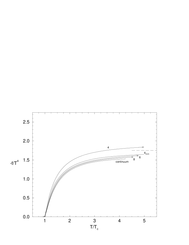
Figure 2: The free energy density $f$ versus $T/T_{c}$ on lattices $16^{3}\times 4$, $32^{3}\times 6$ and $32^{3}\times 8$ with the Wilson action [7] (curves labeled with 4, 6 and 8) and on lattice $24^{3}\times 4$ with the $2\times 2$ Symanzik–improved action [19] (curve labeled with $4_{(2\times 2)}$). The lower curve is the extrapolation to $N_{\tau}\rightarrow\infty$ obtained from the curves with $N_{\tau}=6$ and 8. The horizontal dashed line indicates the ideal gas continuum value.

In Fig. 2, the present situation for lattice determinations of the free energy density in finite temperature SU(3) gauge theory is summarized.

4 Monte Carlo results

In this Section, the free energy density of finite temperature SU(3) gauge theory is determined at temperatures $T/T_{c}=4/3,3/2$ and 2 on lattices with $N_{\tau}=2,3$ and $N_{\sigma}=4N_{\tau}$, adopting the parametrized FP actions of two different RG transformations. The first one is the type I RG transformation defined in Ref. [13]; the second one is the new proposal [16] – type III RG transformation. Both actions are parametrized in terms of powers of the real part of the trace of the plaquette and of the twisted perimeter–six loop (i.e the loop defined by the path $\hat{x}\hat{y}\hat{z}$-$\hat{x}$-$\hat{y}$-$\hat{z}$, for example). Given the following form for the parametrization

$$A(U)=\frac{1}{N}\sum_{C,\ i\geq 1}c_{i}(C)[N-{\rm ReTr}(U_{C})]^{i}\;\;\;,$$ (13)

where the sum is over all the closed paths which define a plaquette or a twisted loop and $U_{C}=\Pi_{C}U_{\mu}(n)$, the couplings $c_{i}(C)$, $i=1,\ldots,4$, are determined in order to approximate the FP action on a large set of configurations (for details, see Refs. [15, 16]). They are summarized in Table 1.

Table 1: Couplings of the parametrized FP action (13) for the RG transformations of type I [15] and type III [16].

		$c_{1}$	$c_{2}$	$c_{3}$	$c_{4}$
type I	plaquette	0.523	0.0021	0.0053	0 .0167
	twisted	0.0597	0.0054	0.0051	–0.0006
type III	plaquette	0.4822	0.2288	–0.1248	0.0228
	twisted	0.0647	–0.0224	0.0030	0.0035

According to Eq. (12), the lattice determination of the free energy density at a temperature $T$ calls first for the calculation of expectation values of the action density on lattices $N_{\sigma}^{4}$ and $N_{\sigma}^{3}\times N_{\tau}$ for a sufficiently large set of $\beta$’s and then for an integration up to the value of $\beta$ corresponding to the temperature $T$ at a fixed $N_{\tau}$.

The usual procedure to determine the correspondence between the coupling $\beta$ and the temperature $T$ at a fixed $N_{\tau}$ needs a non–perturbative determination of $a(\beta)$ or, equivalently, of the $\beta$–function. This procedure usually involves an interpolation of numerical data (see the previous Section). Since the central point of this paper is to single out lattice cut–off effects of FP actions, an alternative way which introduces no additional artificial effects has been exploited. The idea is that the critical coupling $\beta_{c}(N_{\tau}^{\prime})$ on a lattice with $N_{\tau}^{\prime}$ sites in the time direction and infinite spatial volume corresponds to the physical temperature $T=(N_{\tau}^{\prime}/N_{\tau})T_{c}$ on a lattice with $N_{\tau}$ sites in the time direction. Indeed, starting from the definition of the critical coupling $\beta_{c}(N_{\tau}^{\prime})$

$$T_{c}\;=\;\frac{1}{N_{\tau}^{\prime}a(\beta_{c}(N_{\tau}^{\prime}))}\;\;\;,$$ (14)

it is easy to see that it corresponds to the temperature

$$T\;=\;\frac{1}{N_{\tau}a(\beta_{c}(N_{\tau}^{\prime}))}\;=\;\frac{N_{\tau}^{\prime}}{N_{\tau}}T_{c}$$ (15)

on a lattice with temporal extent $N_{\tau}$. The advantage of this procedure is that critical couplings can be determined with high precision. The drawback is, of course, that only discrete sets of temperatures can be determined.

For the type I FP action, the critical couplings on lattices with $N_{\tau}=2,3,4,6$ were already determined in Ref. [15]; for the type III FP action the same work has also been done [16]. In Table 2, results for both actions have been summarized.

Table 2: Critical couplings at finite volume and extrapolated to infinite volume for the FP actions type I and III parametrized as in Table 1.

	volume	$N_{\tau}=2$	$N_{\tau}=3$	$N_{\tau}=4$	$N_{\tau}=6$
type I	$4^{3}$	2.89(1)
	$6^{3}$	2.945(15)	3.320(15)
	$8^{3}$	2.96(1)	3.34(1)	3.50(1)
	$10^{3}$	2.960(5)	3.34(1)	3.51(1)	3.78(2)
	$12^{3}$	2.975(5)	3.343(5)	3.520(5)	3.775(5)
	$15^{3}$				3.777(5)
	$18^{3}$				3.790(5)
	infinite	2.976(5)	3.345(5)	3.520(5)	3.790(6)
type III	$4^{3}$	3.361(5)
	$5^{3}$	3.378(3)
	$6^{3}$	3.385(9)	3.568(4)
	$8^{3}$	3.395(3)		3.678(3)
	$9^{3}$		3.581(4)
	$10^{3}$	3.399(5)		3.686(3)	3.91(4)
	$12^{3}$		3.587(5)	3.691(5)	3.87(1)
	$14^{3}$			3.691(5)	3.882(7)
	$16^{3}$				3.882(8)
	infinite	3.400(3)	3.588(4)	3.695(4)	3.885(13)

According to Eq. (15) and making use of infinite volume extrapolations in Table 2, the $\beta$ couplings corresponding to temperatures the $T/T_{c}=3/2,2$ and 3 on a lattice with $N_{\tau}=2$ and those corresponding to temperatures $T/T_{c}=4/3$ and 2 on a lattice with $N_{\tau}=3$ can be singled out, for both type I and type III FP actions.

In this paper, simulations have been performed on lattices with $N_{\tau}=$ 2 and 3 and with the ratio $N_{\sigma}/N_{\tau}$ fixed to 4 in order to rule out finite size effects. The simulation algorithm adopted was a mixture of four sweeps of a 20–hit Metropolis and one sweep of an over–relaxation consisting in four updates of SU(2) subgroups. With the same algorithm, the Wilson action would take $\sim 7$ times less for a sweep [15].

The free energy density was determined according to Eq. (12) at temperatures $T/T_{c}=3/2$ and 2 on the lattice with $N_{\tau}=2$ and at temperatures $T/T_{c}=4/3$ and 2 on the lattice with $N_{\tau}=3$. This allows to compare the results at $T/T_{c}=2$ obtained on lattices with different $N_{\tau}$ and to check the amount of cut–off effects. In Figs. 3, 4 and 5, the quantity $\Delta S=N_{\tau}^{4}(\langle S_{0}\rangle-\langle S_{T}\rangle)$ for a large range of $\beta$ is plotted for the Wilson action with $N_{\tau}=2$ and for the type III FP action with $N_{\tau}=2$ and 3, respectively. In the case of the type I FP action the qualitative behavior is the same as for the type III FP action. In all three cases the action density shows a rapid variation at the critical coupling, which is smoother on the smaller lattices. The time history of the runs for $\langle S_{T}\rangle$ in the transition region clearly shows flips between two phases, as expected for a first order phase transition.

For the calculation of the free energy density, $\Delta S$ has to be integrated with respect to $\beta$. For this purpose, a spline fit interpolation of the data for $\Delta S$ was first performed. As an estimate of the uncertainty in the integration coming from the interpolation procedure, a straight line interpolation was also considered. Although careful checks have been done in the time histories of the runs for $S_{T}$ in the transition region, the possibility of a (small) systematic error induced by hysteresis effects cannot be excluded. In Table 3 all the results for $-f/T^{4}$ found in this work are summarized.

Table 3: Values of $f/T^{4}$ at physical temperatures $T/T_{c}=4/3,3/2,2$ on lattices with $N_{\tau}=2$ and 3 for the type I and III FP actions and with $N_{\tau}=2$ for the Wilson action.

	lattice	$T/T_{c}=4/3$	$T/T_{c}=3/2$	$T/T_{c}=2$
type I	$8^{3}\times 2$		1.2226(6)	1.528(4)
	$12^{3}\times 3$	0.769(10)		1.350(10)
type III	$8^{3}\times 2$		1.0805(23)	1.3279(24)
	$12^{3}\times 3$	0.733(11)		1.221(10))
Wilson	$8^{3}\times 2$		2.2007(8)	2.5652(7)

In Fig. 6 the results for the type III FP action are compared with previous determinations with the Wilson action [7] and the Symanzik–improved action [19], together with the continuum limit extrapolation [7]. The horizontal error bars represent the uncertainty in the determinations of the physical temperature $T/T_{c}$ coming from the uncertainty in the measurements of the critical couplings. They have been estimated imposing the independence of the critical temperature $T_{c}$ on the critical couplings for the various $N_{\tau}$’s and using the ansatz $a\Lambda_{L}=f(\beta)|_{2-loop}\cdot\lambda(\beta)$, where $\lambda(\beta)$ is a smooth function satisfying $\lambda(\beta\rightarrow\infty)=1$.
At $N_{\tau}=2$ there are results for $-f/T^{4}$ at $T/T_{c}=3/2$ and $T/T_{c}=2$: while the Wilson action shows $O(100\%)$ cut–off effects, the type III FP action gives values differing from the continuum values estimated in [7] by $\sim 24\%$ at $T/T_{c}=3/2$ and by $\sim 9\%$ at $T/T_{c}=2$.
At $N_{\tau}=3$, the result for $-f/T^{4}$ with the type III FP action at $T/T_{c}=4/3$ differs from the continuum by $\sim 10\%$ and at $T/T_{c}=2$ is consistent with the continuum value.

Although the global scenario exhibits an evident improvement with respect to the approach with the standard actions, it is worth to make some comments on the surviving cut–off effects in the results of the FP actions. The qualitative understanding of such cut–off effects is straightforward. Recalling the classification at the end of Section 2, the effect mentioned in i. should explain the deviations between $N_{\tau}=2$ and $N_{\tau}=3$ results; the effect mentioned in ii. can be responsible of the cut–off effects at small $\beta$ – and so at small $T$ – for each $N_{\tau}$; the effect mentioned in iii. can overlap to the previous one at small $\beta$, where the parametrization of the FP action is more likely to fail to reproduce the true FP action. It would be interesting to evaluate quantitatively the contribution of the different sources of cut–off effects: if one of them is largely dominating, it can be removed by an ad hoc strategy.

5 Acknowledgements

I thank P. Hasenfratz (who suggested this subject), M. Blatter, G. Boyd, F. Farchioni, F. Karsch and F. Niedermayer for many useful discussions. I am indebted to P. Hasenfratz and F. Niedermayer for the Monte Carlo code of the FP actions.

Figure 3: $\Delta S\equiv N_{\tau}^{4}(\langle S_{0}\rangle-\langle S_{T}\rangle)$ versus $\beta$ for the Wilson action on a lattice $8^{3}\times 2$ lattice. The vertical lines represent the critical couplings and the related errors on lattices $8^{3}\times 2$ [20], $12^{3}\times 3$ [21] and $\infty^{3}\times 4$ [7], respectively from left to right.

Figure 4: $\Delta S\equiv N_{\tau}^{4}(\langle S_{0}\rangle-\langle S_{T}\rangle)$ versus $\beta$ for the type III FP action on a $8^{3}\times 2$ lattice. The vertical lines represent the critical couplings and the related errors on lattices $8^{3}\times 2$, $\infty^{3}\times 3$ and $\infty^{3}\times 4$, respectively from left to right (see Table 2).

Figure 5: $\Delta S\equiv N_{\tau}^{4}(\langle S_{0}\rangle-\langle S_{T}\rangle)$ versus $\beta$ for the type III FP action on a $12^{3}\times 3$ lattice. The vertical lines represent the critical couplings and the related errors on lattices $12^{3}\times 3$, $\infty^{3}\times 4$ and $\infty^{3}\times 6$, respectively from left to right (see Table 2).

Figure 6: The same as in Fig. 2 with the addition of the results of this work for the Wilson action and the type III FP action (see Table 3). The vertical dotted lines corresponding to $T/T_{c}=4/3,3/2$ and 2 are drawn to guide the eyes.

References

- [1] A. Linde, Phys. Lett. B96 (1980) 289.
- [2] P. Arnold and C.-X. Zhai, Phys. Rev. D50 (1994) 7603.
- [3] C.-X. Zhai and B. Kastening, Phys. Rev. D52 (1995) 7232.
- [4] K.G. Wilson, Phys. Rev. D10 (1974) 2445.
- [5] J. Engels, F. Karsch and K. Redlich, Nucl. Phys. B435 (1995) 295.
- [6] B. Beinlich, F. Karsch and E. Laermann, Nucl. Phys. B462 (1996) 415.
- [7] G. Boyd, J. Engels, F. Karsch, E. Laermann, C. Legeland, M. Lütgemeier and B. Petersson, Phys. Rev. Lett. 75 (1995) 4169; “Thermodynamics of SU(3) Lattice Gauge Theory”, Bielefeld–preprint BI–TP 96/04, hep–lat/9602007.
- [8] F. Karsch, “Lattice regularized QCD at Finite Temperature”, Lectures given at the “Enrico Fermi School”: Selected Topics in non perturbative QCD, Varenna (Italy) 1995, Bielefeld–preprint BI–TP 95/38, hep–lat/9512029.
- [9] K. Symanzik, in New developments in gauge theories, ed. G. ’t Hooft (Plenum New York, 1980); in Lecture Notes in Physics, 153, ed. R. Schrader et al. (Springer, Berlin, 1982); in Non–perturbative field theory and QCD, ed. R. Jengo et al. (World Scientific, Singapore, 1983); K. Symanzik, Nucl. Phys. B226 (1983) 187 and 205.
- [10] P. Hasenfratz and F. Niedermayer, Nucl. Phys. B414 (1994) 785; see also: P. Hasenfratz, Nucl. Phys. B (Proc. Suppl.) 34 (1994) 3; F. Niedermayer, ibid. 513.
-
[11]
K.G. Wilson and J. Kogut, Phys. Rep. C12 (1974) 75;
K.G. Wilson, Rev. Mod. Phys. 47 (1975) 773; ibid. 55 (1983) 583. - [12] K.G. Wilson, in Recent developments of gauge theories, ed. G. ’t Hooft et al. (Plenum, New York, 1980).
- [13] T. DeGrand, A. Hasenfratz, P. Hasenfratz and F. Niedermayer, Nucl. Phys. B454 (1995) 587.
- [14] F. Farchioni, P. Hasenfratz, F. Niedermayer and A. Papa, Nucl. Phys. B454 (1995) 638.
- [15] T. DeGrand, A. Hasenfratz, P. Hasenfratz and F. Niedermayer, Nucl. Phys. B454 (1995) 615.
- [16] M. Blatter and F. Niedermayer, “New fixed point action for SU(3) lattice gauge theory”, Bern–preprint, BUTP–96/12.
- [17] J. Engels, J. Fingberg, F. Karsch, D. Miller and M. Weber, Phys. Lett. B252 (1990) 625.
- [18] K. Akemi et al., Phys. Rev. Lett. 71 (1993) 3063.
- [19] B. Beinlich, Diploma thesis, Bielefeld 1996.
- [20] B.J. Pendleton, in Gauge Theory on a Lattice: 1984, ed. C. Zachos et al. (CONF–8404119, Argonne, 1984)
- [21] J. Fingberg, U. Heller and F. Karsch, Nucl. Phys. B392 (1993) 493.