KEK-CP-045

April 1996

STRINGS IN COMPUTER

H.Kawai, N.Tsuda, and T.Yukawa

^{† ‡} National Laboratory for High Energy Physics (KEK)

Tsukuba, Ibaraki 305 , Japan

^§ Coordination Center for Research and Education,

The Graduate University for Advanced Studies,

Hayama-cho, Miura-gun, Kanagawa 240-01, Japan

and

National Laboratory for High Energy Physics (KEK)

Tsukuba, Ibaraki 305, Japan

Complex structures are determined for surfaces with $S^{2}$ and $T^{2}$ topologies generated by the dynamical triangulation method. For a surface with $S^{2}$ topology the spacial distribution of the conformal mode is obtained, while for the case of $T^{2}$ topology the distribution of the moduli parameter is calculated. It is also shown that the network of Feynman diagrams of massive $\phi^{3}$ scalar theory has a unique complex structure. This gives a numerical justification of the hadronic string model for explaining the n-particle dual amplitude.

1 Complex structure in the Polyakov string

For quantizing the Polyakov string one usually considers a set of closed string world sheets of the 2-dimensional Euclidean space-time[1]. Each world sheet is considered to be a closed and orientable manifold with various topology. Once the Riemannian metric $g_{ab}$ is given on this manifold, it is always possible to introduce a complex structure on the surface. For example, the Riemannian metric of a surface with $S^{2}$ topology can be written by a suitable choice of local coordinates as

$$g=g_{ab}dx^{a}dx^{b}=e^{\sigma(z)}dzd{\bar{z}},$$

where $z=x+{\rm i}y$, and $e^{\sigma(z)}$ is the conformal factor. Therefore the problem of quantizing two-dimensional gravity is reduced to considering the quantum fluctuations of the conformal mode and the complex structure. This is the basic assumption one usually employs in the Liouville field theory of non-critical Polyakov string.

Now, we would like to examine this assumption constructively, by determining the complex structure for those surfaces obtained numerically by the dynamical triangulation(DT). The Monte Carlo simulation of the random surface by the DT method[2] has been regarded as a numerical exercise of the matrix model[3] which is known to give the correct critical exponent identical to the continuous field theory, i.e. the Liouville field theory[4]. In what follows we shall show that the DT method also exhibits its explicit correspondence to the continuous field theory in the sense that those surfaces created by DT numerically can be decomposed to a unique complex structure and conformal mode[5].

2 The basic idea -resistivity-

Our method is based on the observation that the resistance of a homogeneous conducting sheet is invariant under the local scale transformation. This can be shown by considering the resistance of a small rectangular section with length $a$ and width $b$ of a conducting sheet. The resistance between two sides of length $a$ is given by

$$R=r{a\over b},$$

where $r$ is the resistivity constant. The resistance $R$ is apparently invariant under the scale change $a\mapsto a\eta$, $b\mapsto b\eta$. Therefore, the local scale factor does not affect the resistance.

Figure 1: Resistivities for the case of pure gravity. The size of ($a$), ($b$) and ($c$) are $4000$, $8000$ and $16000$ triangles respectively.

Figure 2: Resistivities for the case of 2 scalars.

Experimentally, the resistance measurement of a conducting sheet is carried out by picking up four points on the surface which we specify by four complex numbers $\{z_{i}\}$. With a source of current $I$ placed at $z_{3}$ and a sink of the current at $z_{4}$ the voltage drop from a point $z_{1}$ to a point $z_{2}$ is written as

$$V(z_{1})-V(z_{2})=R(z_{1},z_{2};z_{3},z_{4})I.$$

In the case of surface with $S^{2}$ topology it can be regarded as an infinite flat sheet and we obtain from Gauss’ law

$$R=-{r\over 2\pi}\ln|[z_{1},z_{2};z_{3},z_{4}]|,$$

where

$$[z_{1},z_{2};z_{3},z_{4}]={z_{1}-z_{3}\over z_{2}-z_{3}}{z_{2}-z_{4}\over z_{1}-z_{4}}$$

is known as the anharmonic ratio.

We regard the dual graph of a triangulated surface as a trivalent network of registers each having $1\Omega$. We pick up two vertices for applying current with $1A$, and solve the Kirchhoff equation by the Jacobi iteration method. Then, we measure voltage drops between other pair of vertices. Using the $SL(2,C)$ transformation,

$$z\mapsto{az+b\over cz+d}(ad-bc=1),$$

invariance property of the anharmonic ratio we can fix three points among $\{z_{i}\}$ at $z_{3}=0$,$z_{4}=\infty$ and $z_{2}=1$ without changing the resistance by an appropriate choice of four complex parameters $(a,b,c,d)$. In practice, among $4!$ combinations of measuring arrangements there are known to be only two independent measurements, while we have three unknowns, namely one complex $z_{1}$ and one real $r$. In order to fix them unambiguously we add one more measuring point $z_{5}$.

Figure 3: Resistivities for the case of 3 scalars.

3 Complex structure of $S^{2}$ surfaces

Let us show results of the resistivity measurement for random surfaces with $S^{2}$ topology simulated by the DT method with $N$ triangles. If a conducting surface is uniform and homogeneous, we should get a fixed resistivity regardless of points of measurements. Fig.1 shows the distributions of resistivity constant for surfaces of three area sizes with no matter fields coupled(the pure gravity). The distributions peak at about $r=2.6$ and they get sharper as the size grows. Broader distributions in small surface simulations reflect the mesh structures of circuit networks, and we can expect that the peak will eventually become the $\delta$-function type distribution as the area get infinity. On the contrary, when surfaces are coupled with matter fields with the central charge $c$ bigger than 1, peaks of the resistivity distribution tend broader as the size grows.

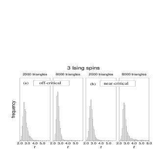
Figure 4: We plot resistivities for 3 Ising spins both case of off-critical $(a)$ and near critical $(b)$.

Fig.2($c=2$) and Fig.3($c=3$) show the tendency clearly. This phenomenon suggests the absence of a unique continuous limit for cases $c>1$ as expected from analytic theories. The $c=1$ barrier can be seen more significantly in the measurement of a surface with three Ising spins coupled(Fig.4). It should behave as a system with the $c={3\over 2}$ matter coupled at the critical point, while it is expected to be in the same universality class as the pure gravity off the critical point. Indeed, our measurement shows this behavior. Broadening of the resistivity for bigger size naturally implies the transition of the surface to the branched polymer phase beyond $c=1$.

4 Distribution of the conformal factors

Once we obtain the resistivity $r$ for a surface, we can locate the position of each triangle by two measurements of resistances, for example

$$R(z_{1},1;0,\infty)=-{r\over 2\pi}\ln|z_{1}|,$$

and

$$R(z_{1},0;1,\infty)=-{r\over 2\pi}\ln|1-z_{1}|.$$

By sweeping all the rest of triangles with fixing three points which correspond to $(1,0,\infty)$, we can determine the position of all the triangles of this surface. The point density obviously represents the distribution of conformal factors proportional to

$$\lim_{z_{4}\to\infty}|z_{4}|^{4}<e^{\alpha\sigma(0)}e^{\alpha\sigma(1)}e^{\alpha\sigma(z_{4})}e^{\alpha\sigma(z_{1})}>.$$

In Fig.5 we show the distribution of triangles whose position $z$ is mapped within a circle by the transformation

$$z\mapsto{az\over z+a-1}$$

with $a={1\over 2}+i{{\sqrt{3}}\over 2}$.

Figure 5: A plot of the obtained coordinates of all vertices for $c=0$ with five independent configurations superimposed. As a matter of convenience all points are mapped into a circle with the center at ($\frac{1}{2},\frac{\sqrt{3}}{2}$) and radius $\frac{\sqrt{3}}{3}$.

There exists a theoretical prediction of the distribution[6], but it has not been presented in a form ready for the direct comparison to the numerical experiments.

5 Complex structure of the $T^{2}$ surface

As far as two dimensional orientable manifolds of $S^{2}$ topology are concerned they all have the same complex structure, i.e. any manifold can be transformed to the other by a combination of a general coordinate transformation(Diffeo) and the Weyl transformation(Weyl). On the other hand for the surface with $T^{2}$ topology the moduli space

$$\{g_{ab}\}/Weyl\otimes Dif\!feo$$

is spanned by a complex plane of moduli $\tau$. It is defined by the ratio of the integrals of an Abelian differential

$$\tau={\oint_{b}j_{\mu}dx^{\mu}+i\oint_{b}{\tilde{j}}_{\mu}dx^{\mu}\over\oint_{a}j_{\mu}dx^{\mu}+i\oint_{a}{\tilde{j}}_{\mu}dx^{\mu}},$$

where integration contours (we call them as the a-cycle and the b-cycle) are chosen to be two closed paths on the manifold which cross each other only once. Here, $j_{\mu}dx^{\mu}$ is a harmonic $1$-form and $\tilde{j}_{\mu}dx^{\mu}$ is its dual. If we regard $j_{\mu}$ as a current density on the torus, $r\oint_{a}j_{\mu}dx^{\mu}$ and $\oint_{a}{\tilde{j}}_{\mu}dx^{\mu}$ correspond to the voltage drop along the a-cycle and the total current crossing the a-cycle, respectively.

In practice, we select two closed paths made up by connecting edges of triangles, which intersect only once. Then we cut the surface along one of the path for which we choose the b-cycle, and apply constant voltages(1V) in between neighbouring triangles dual to the cut(Fig.6).

Figure 6:

Solving the Kirchhoff equation we can determine all the currents $j_{\mu}$ and ${\tilde{j}}_{\mu}$ along links between neighbouring triangles in the dual graph. By construction of the network the following two integrals are trivial;

$$\oint_{a}j_{\mu}dx^{\mu}={1\over r},\oint_{b}j_{\mu}dx^{\mu}=0.$$

Thus $\tau$ is obtained by measuring total currents crossing two cycles;

$$\tau=\frac{iI_{b}}{\frac{1}{r}+iI_{a}}$$

where $I_{a}$ and $I_{b}$ represent the total currents crossing the a-cycle and the b-cycle, respectively. Instead of measuring the resistivity of this surface we employ the value determined previously for the surface with $S^{2}$ topology and corresponding central charge.

Figure 7: Plot of the moduli($\tau$) on the complex-plane mapped to the fundamental domain with a total number of triangles of $4,000$ and $8,000$. Each dot corresponds to the moduli$\tau$ for a sample of DT-surface.

Fig.7 shows the distribution of $\tau$ for configurations of 4,000 and 8,000 triangles. Each value of $\tau$ is transformed appropriately by the $SL(2,Z)$ transformation

$$\tau\mapsto{a\tau+b\over c\tau+d}\;\;\;(ad-bc=1)$$

so that it is in the fundamental domain. By summing over real $\tau$’s with a fixed imaginary part we get the distribution for surfaces with two, four and eight thousand triangles in Fig.8, which should be compared with the theoretical prediction

$$({\rm Im}\tau)^{-{3\over 2}}e^{-{\pi\over 6}{\rm Im}\tau}\left|\prod_{n=1}^{\infty}(1-e^{2\pi i\tau n})\right|^{-2}.$$

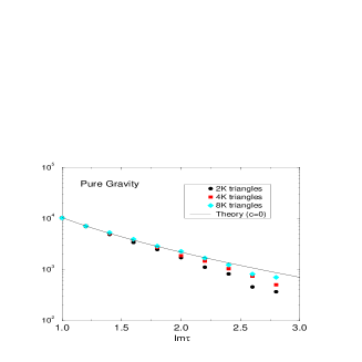
Figure 8: Four density-distributions(histogram) of imaginary part of moduli $\tau_{2}$ for the case of pure-gravity with the topology of the torus. These are obtained by integrating over of the real part of moduli $\tau_{1}$ on the complex plane. A scale of vertical line is arbitrary.

The Liouville theory predicts for a surface with c scalar fields

$$({\rm Im}\tau)^{-{c+3\over 2}}e^{{\pi\over 6}(c-1){\rm Im}\tau}\left|\prod_{n=1}^{\infty}(1-e^{2\pi i\tau n})\right|^{-2(c-1)},$$

i.e. for simulations with $c>1$ matter the surface will be unstable to the polymer like torus configuration in the limit ${\rm Im}\tau\rightarrow\infty$.

6 Hadronic strings -a root of the string model-

Figure 9:

The n-particle amplitudes of the massive $\phi^{3}$ scalar theory corresponding to the diagram $G$ shown by Fig.9 is given by

$$I_{G}(p_{1},p_{2},...,p_{n})=\int\prod^{N_{1}}_{i=1}d^{D}q_{i}\prod^{N_{1}}_{i}{1\over q^{2}_{i}+m^{2}}\prod^{N_{0}}_{a=1}\delta(P_{a}),$$

where $P_{a}$ is the net momentum flowing into the vertex $a$. Here, $N_{0}$ stands for the total number of vertices, and $N_{1}$ for the total number of internal lines. By the Laplace transform of a propagator,

$${1\over q^{2}_{i}+m^{2}}=\int^{\infty}_{0}d\alpha_{i}e^{-\alpha_{i}(q_{i}^{2}+m^{2})},$$

the amplitude is expressed after integrated over $\{q_{i}\}$ as

$$I_{G}=\int\prod_{i}^{H_{1}}d\alpha_{i}\alpha_{i}^{-{D\over 2}}e^{-\sum\alpha_{i}m^{2}}\int\prod_{a}^{N_{0}}d^{D}x_{a}{\rm exp}\{-{1\over 4}\sum_{i}{(x_{a(i)}-x_{b(i)})^{2}\over\alpha_{i}}\}e^{i\sum_{a}^{N_{0}}x_{a}p_{a}},$$

where $a(i)$ and $b(i)$ are two vertices connected by the propagator $i$. This equation has been often noticed on its resemblance to the electric circuit[7],i.e.

$$\alpha_{i}\rightarrow{\rm resister},x_{a}\rightarrow{\rm voltage},p_{a}\rightarrow{\rm current}.$$

Then, $Q={1\over 4}\sum{(x_{a(i)}-x_{b(i)})^{2}\over\alpha_{i}}$ is regarded as the total heat generated by the circuit. It has been conjectured that as the mesh becomes finer the surface will tend to be a uniform, homogeneous and continuous conductor. In this case after averaging over all n-particle diagrams we will obtain

$$<I>\sim e^{-{1\over 2}\sum_{a,b}R_{ab}({\bar{\alpha}})p_{a}p_{b}},$$

where ${\bar{\alpha}}$ is an appropriate resistivity of the surface and the resistance is same as that of the flat conductor;

$$R_{ab}\propto\ln|z_{a}-z_{b}|$$

.

We have made the measurement of resistivity for networks with $S^{2}$ topology constructed by the same DT method as described previously. This time each link has resistance distributed randomly with the probability

$$\alpha^{-{D\over 2}}e^{-\alpha m^{2}}.$$

Here, we have chosen the parameters to be $D=0$ and $m=1$ in the simulation.

Figure 10: Resistivities for the case of pure gravity when each resistance is randomly distributed.

Fig.10 shows the size dependence of the resistivity distribution. As the size gets larger the distribution becomes sharper similar to the case of the pure gravity. This gives a numerical support of the theoretical conjecture.

References

- [1] A.M.Polyakov, Phys.Lett. B103 (1981) 207.
- [2] D.Weingarten, Nucl.Phys.B210(1982)229; F.David, Nucl.Phys. B257[FS14] (1985) 45; V.A.Kazakov, Phys.Lett. B150 (1985) 282; J.Ambjørn, B.Durhuus and J.Frhlich, Nucl.Phys.B257[FS14] (1985) 433; Nucl.Phys.B275 [FS17] (1986) 161.
- [3] E.Brézin and V.Kazakov, Phys.Lett. 236B (1990) 144; M.Douglas and S.Shenker, Nucl.Phys. B335 (1990) 635; D.Gross and A.Migdal, Phys.Rev.Lett. 64 (1990) 127.
- [4] V.G.Knizhnik, A.M.Polyakov and A.B.Zamolodchikov, Mod.Phys.Lett A, Vol.3 (1988) 819; J.Distler and H.Kawai, Nucl.Phys. B321 (1989) 509; F.David, Mod.Phys.Lett. A3 (1988) 1651.
- [5] H.Kawai, N.Tsuda and T.Yukawa, Phys.Lett. B 351 (1995) 162; H.Kawai, N.Tsuda and T.Yukawa, B(Proc. Suppl.) hep-lat/9512014.
- [6] A.B.Zamolodchikov and Al.B.Zamolodchikov het-th/9506136
- [7] J.D.Bjorken and S.D.Drell, McGraw Hill, New York, 1965; H.B.Nielsen and P.Olesen, Phys.Lett. B32 (1970) 203; B.Sakita and M.A.Virasoro, Phys.Rev.Lett. 24 (1970) 1146.