We investigate possible problems with universality in lattice gauge theory where a mixed fundamental SU(2) and SO(3)-invariant gauge group is used: the (second order) finite temperature phase transition becomes involved with first order effects with increased SO(3) coupling, and this first order effect has a noticeable coupling dependence for small lattices. We produce evidence that the first order transition is essentially bulk in nature as generally believed, and that the finite temperature effects start to separate out from the lower end of the bulk effects for a lattice of 8 sites in the finite temperature direction. We strengthen our picture of the first order effects as artefacts by using an improved action: this shifts the end point of the first order line away from the fundamental SU(2) axis.

1 Introduction

If the success of lattice gauge theory is to be measured by the relevance of its results to experiment, we can now fairly claim that a measure of success is finally arriving. Our increased understanding of the simulations and ability to improve them means that we can extract interesting phenomenology.

This paper addresses a more basic worry in the subject: the consistency of the continuum limit in the pure gauge theory. The choice of action is far from unique and one needs to be sure — as a prerequisite for the whole program of lattice gauge theory — that the action one chooses can reproduce the physical limit as the lattice spacing $a$ is taken to zero. Even when one decides (for simulational convenience) on the Wilson form of the action, there is still an ambiguity with regards to the representation of the gauge group. This matter was investigated and largely concluded more than a decade ago.

However, the subject was re-opened recently [1, 2] when it was found that in one version of the SU(2) theory with couplings in mixed representations the deconfining transition — surely a truly physical effect if that claim can ever be made for the pure gauge theory — was apparently mixed in with what had long been known as artefacts of strong coupling.

This appears as a more fundamental problem than simply making the continuum limit hard to obtain: if there is no clear separation between the effects, one can never quite be sure that one’s model represents the physical theory sought. In fact, two of the authors of those papers have recently speculated [3] that the nature of the deconfining transition in SU(2), which was thought to have been settled, may be under threat.

Since it is our intention in this paper to clarify what is, and what is not, a physical effect which will survive the continuum limit, we spend a certain amount of time in the next section explaining the previous results concerning the bulk transitions (an introduction to the early work on the subject is given in reference [4]). We emphasise that, while these effects are not physical as far as the underlying gauge theory is concerned, they are nevertheless not a hindrance to a well-defined continuum limit. We then introduce the new problem with the deconfining transition.

In the following section, we present results from new simulations in a (similar but not identical) variant of the theory aimed at clarifying the position. Finally, we attempt to draw all the results together and suggest there is no danger to the continuum limit.

We should note straight away that we are using the word ‘artefact’ to denote anything obscuring the physics of the continuum limit of the gauge theory in which one is interested; we are not necessarily claiming that the other effects are uninteresting in their own right. We use the words ‘physical’ and ‘physically’ with similar thoughts in mind. Further, we recognise that any such artefacts are a sign that we are still far from the continuum limit; here we must inevitably plead the excuse of finite computing resources.

A brief outline of early results has appeared in [5]; our investigations here are more detailed and our conclusion is different.

2 The mixed action theory

The Wilson action is very widely used in lattice gauge theory as the basis for simulations because of the elegant and simply way it retains gauge invariance in the discrete theory:

$$S_{W}\equiv-\beta_{\mathrm{rep}}\sum_{\Box}\operatorname{Tr}_{\mathrm{rep}}U(\Box)$$ (1)

in which $\beta_{\mathrm{rep}}$ is proportional to the reciprocal of the bare coupling squared and the sum is over all plaquettes (closed loops of the smallest possible size: we use the symbol $\Box$ throughout to represent a plaquette) on the lattice. The variable $U(\Box)$ is the element of the gauge group corresponding to this path.

The point here is that one must make a choice of the representation in which one takes the trace of the group-valued $U(\Box)$. The fundamental representation is the most natural, as it corresponds to the matrices with which one actually implements the theory computationally and is also the representation usually associated with fermions. (There is then a conventional factor of $1/N$ in the trace for SU(N).)

However, in the continuum the theory does not involve elements of the gauge group at all: it is defined in terms of a Lie algebra. The gauge elements were introduced as a useful way of keeping track of gauge invariance, reducing it to nothing more than the linear matrix algebra which is so natural for a computer. Therefore, in the pure gauge theory at least, one should not be restricted to the fundamental representation; one should obtain the same continuum theory from any representation as the cut-off is removed. We shall refer to this in the current paper as universality. In general, the question of universality refers much more widely to independence of the continuum limit from the form of the discretisation, which depends on a great many details; here we concern ourselves only with the particular restricted form. We must also recognise that on any finite lattice, two distinct formulations are highly unlikely to be identical. Nonetheless, as we shall describe, there is a clear sense in which the theories we are dealing with have the same continuum limit.

Let us now specialise to the pure gauge theory with gauge group SU(2), in which the fundamental representation is ‘spin-$1/2$’, to use the familiar language. The group theoretical argument suggests that we could just as well take the adjoint (spin-1) representation and still see the same physics. This representation does not show the full SU(2) invariance. The gauge manifold is a three-sphere $S^{3}$; the adjoint representation is insensitive to factors of $\pm 1$ (corresponding to the center Z(2) of the gauge group), so that opposite ends of diameters on $S^{3}$ should be identified. The actual invariance shown is that of the gauge group SO(3): more generally, this is true of all the whole-integer spin representations of SU(2), while the half-odd-integer representations faithfully reproduce the full invariance. (We shall use the somewhat loose terminology ‘SO(3)-’ and ‘full SU(2)-invariant’ where appropriate to distinguish these cases.) This matter of differing topology will turn out to be crucial.

The first surprise [6] was that the SO(3)-invariant theory turned out to have a strong first order transition not seen in the full SU(2) theory. We return to this below.

It was noticed by Bhanot and Creutz [8] that one could combine different representations of SU(2) (say, the fundamental and adjoint) linearly into the same action, producing a two-dimensional parameter space which would enhance one’s ability to test universality:

$$S_{M}\equiv-\frac{\beta_{F}}{2}\sum_{\Box}\operatorname{Tr}_{F}U(\Box)-\frac{\beta_{A}}{3}\sum_{\Box}\operatorname{Tr}_{A}U(\Box)$$ (2)

with obvious notation and the conventional normalising factors. The SO(3)-invariance of the adjoint term manifests itself as a squaring of the trace of the matrix representing $U(\Box)$; $\operatorname{Tr}_{A}\sim(2\operatorname{Tr}_{F})^{2}-1$. Naively, one would define a combined coupling $\beta_{\mathrm{eff}}=\beta_{F}/4+2\beta_{A}/3$: then in the regime where lattice effects were negligible a physical theory would arise depending only on this effective coupling.

Bulk transitions

Figure 1: First order, bulk phase transitions found in the mixed fundamental-adjoint SU(2) theory by Bhanot and Creutz [8].

The resulting phase diagram showed that the SO(3) transition extended into the plane from the $\beta_{F}=0$ axis, and combined with another roughly vertical transition; the combined line ended abruptly in the middle of the plane. This is shown in figure 1. (To jump ahead, our conclusion will later be that this is a complete picture of the phase transition artefacts afflicting the gauge theory, so this can be compared with our summary diagram, figure 2.)

It appeared that the transitions were all of a bulk nature, in other words independent of the size of the lattice (although it should be noted that due to the computational limitations of the time the simulations were restricted to $N_{S}^{3}\times N_{T}=4^{4}$ lattices). Thus, the transitions have no physical scale associated with them; as the lattice spacing is taken to zero, and hence from asymptotic freedom the inverse bare coupling $\beta$ is taken to infinity the transitions remain behind at the same fixed coupling. This means that — provided a continuum theory exists at all — they are artefacts of some sort.

There was one clue to the nature of the near-vertical part of the transition: if $\beta_{A}$ is taken to infinity keeping $\beta_{F}$ finite, the fields are forced to $\pm I$ ($I$ is the group identity element), which the adjoint representation does not distinguish. Thus there is an embedded Z(2) theory corresponding to flipping the sign of any element of the gauge group; this becomes an exact symmetry for zero $\beta_{F}$ at all $\beta_{A}$. In the case of $\beta_{A}\to\infty$ for finite $\beta_{F}$, the coupling is just that of a Z(2) gauge model, and the end of the line at $\beta_{A}=\infty$ is just the $Z(2)$ symmetry breaking transition of this model. The coupling in this limit is known analytically to be $\log(1+\sqrt{2})/2\sim 0.4407$, which agrees with the line appearing in the mixed action diagram. Clearly, in this limit the gauge theory no longer plays a part. This leads us to label the line in the diagram as an artefact.

The Villain form

Further work by Caneschi, Halliday, Schwimmer [7, 9] clarified the nature of the SO(3)-like bulk transition. They defined a ‘Villain’ form for the theory, in which the SO(3) invariant part of the action was rewritten to include an auxiliary Z(2)-valued field $\sigma(\Box)$, taking values on plaquettes. The action becomes

$$S_{V}\equiv-\frac{\beta_{F}}{2}\sum_{\Box}\operatorname{Tr}_{F}U(\Box)-\frac{\beta_{V}}{2}\sum_{\Box}\operatorname{Tr}_{F}U(\Box)\times\sigma(\Box)$$ (3)

and the measure is extended to include a sum over ${\sigma(\Box)}={\pm 1}$. The SO(3) invariance is now manifest in this new $Z(2)$ symmetry: for every configuration with a given $U(\Box)=1$, there is another with $U(\Box)=-1$.

If one is probing the differences between the full-SU(2) and SO(3) theories, this form of the action is as good a tool as the fundamental/adjoint form. However, the Villain part does not correspond to an irreducible representation of SU(2): in fact it includes contributions from all representations with integer spin; the expansion is given in reference [7]. The naive effective coupling in this case is simply

$$\beta_{\mathrm{eff}}=\beta_{F}+\beta_{V}.$$ (4)

The phase diagram found is very similar to the fundamental/adjoint one, although the vertical axis has a different scale with the SO(3) phase transition now around $\beta_{V}\sim 4.3$ instead of $\beta_{A}=2.5$ (in fact, this is the only substantial difference between the theories that we have noticed).

Monopoles and charges

The Villain form has both practical advantages (discussed in the next section) and theoretical ones, namely the transparency with which Z(2) effects can be seen in the behaviour of the $\sigma(\Box)$ variables. The behaviour of the SO(3) transition was elucidated in terms of the Z(2) effects in reference [7] and this was extended to the mixed-action plane in reference [9]; this is an expanded and slightly re-interpreted account of the explanations therein.

The Z(2) degrees of freedom can be divided up into two types of object, ‘monopoles’ $M$ and ‘charges’ $E$, defined by

$$\begin{split}M(c)&\equiv\frac{1}{2}\left(1-\prod_{\Box\in\partial c}\sigma(\Box)\right)\\ E(l)&\equiv\frac{1}{2}\left(1-\prod_{\Box\in\hat{\partial}l}\sigma(\Box)\right)\\ \end{split}$$ (5)

in which $c$ is a (three-dimensional) cube and $l$ is a link of the lattice: the monopole is defined as a product of the plaquette-valued Z(2) variable over the faces of the cube $c$ and the charge as the product over all plaquettes having the link $l$ in their perimeter. Each can take the value $1$ or $0$.

In this picture, a cube having $M(c)=1$ contains a monopole; one can draw a Dirac string from it to another cube having $M(c)=1$ by tracing plaquettes with $\sigma(\Box)=-1$.

Considering the special case $\beta_{F}=0$, the charge degrees of freedom are trivial: multiplying $E(l)$ by $-1$ is the same as multiplying the link $U(l)$ by $-1$, so that the gauge variables and the monopoles are sufficient to describe the complete theory. One can alter the values of the charges by flipping the signs of all relevant plaquettes without changing the physical state. As each cube contains exactly two (or zero) plaquettes from a charge $E(l)$, this does not change the value of a monopole either: this corresponds to an unphysical movement of the Dirac string. The authors of reference [9] suggest some dual behaviour between the monopoles and charges in the mixed-action theory.

As the monopole is a Z(2) object, in the gauge theory one can think of it as flipping the sign of a gauge element. This is related to the disconnected nature of the SO(3) gauge manifold; one can transform a gauge element continuously from a value $g$ to $-g$, but as these points are identified this is a closed path which cannot be shrunk to zero. The monopoles are a sign that such closed paths are contributing to the path integral.

Thinking of monopoles as dynamical degrees of freedom, then, at small $\beta_{V}$ entropy effects dominate and monopoles are present. As $\beta_{V}$ increases entropy loses out to minimising the action and the gauge degrees of freedom tend to settle close to the identity. In this second case, the closed paths joining the regions around the identity and its negative are not present, since gauge elements representing plaquettes which lie in between would produce a large action. Hence the regions around the identity and its negative, although images of one another in the pure SO(3) case, appear disconnected when considering the whole three-sphere of the SU(2) manifold: in other words, monopoles are suppressed. The part of the first order transition which survives in the limit $\beta_{F}\to 0$ corresponds to the disappearance of the monopoles.

If monopoles are suppressed in the charge-independent pure SO(3) theory, then in the second term of equation 3 we are left with only $\beta_{V}\operatorname{Tr}_{F}U(\Box)$, identical to the fundamental theory. It was indeed found by Halliday and Schwimmer [7] that the monopoles were strongly suppressed in the high-$\beta_{V}$ phase; thus the continuum limit of the SO(3) theory is expected to be the same as that of SU(2) once the phase transition is passed (though the approach to the continuum may be different due to residual monopole effects).

Including the other piece of information about the bulk transitions, namely the Z(2) gauge model limit, the nature of the boxed-in corner of the mixed-action phase diagram becomes clearer. The Z(2) symmetry which was manifest for the charges in the SO(3) theory survives with increasing $\beta_{F}$ out to the first order phase transition and is then broken.

Understanding the first order effects

Here we summarise what the monopole/charge picture tells us about the bulk transitions. It is to be remembered that we are everywhere talking about the bare degrees of freedom, i.e. those defined directly on the lattice, rather than the physical fields for which the picture can be very different.

One can distinguish the upper left corner of the mixed action diagram from the rest of the plane by the following: there, the underlying gauge system occurs around the identity $I$ of SU(2) as well as an image around $-I$. In this region there are no gauge elements lying near the ‘equator’ of the gauge manifold because the action for that is too great, so topologically non-trivial closed paths are not important. The two systems around $I$ and $-I$ are related by an exact Z(2) symmetry for $\beta_{F}=0$; the Monte Carlo results show that the effect of this symmetry persists to finite $\beta_{F}$.

In the rest of the mixed-action plane, there is only one gauge system rather than the two images. For increasing $\beta_{F}$, this is simply the usual theory localised more and more around the identity. In the special case $\beta_{F}=0$ for $\beta_{V}$ below the monopole transition, there is still only one gauge system, but the fields are spread over the whole manifold of the group: increasing $\beta_{F}$ causes a smooth breaking of the Z(2) symmetry.

Thus, in whatever direction we choose to take the continuum limit, we have a smooth transition to the perturbative regime either around $\pm I$ or $I$ alone. The only exception is the limit $\beta_{V}\to\infty$ with $\beta_{F}$ finite. This is pathological because one is effectively tuning away the gauge system leaving only the Z(2) variables; in every other direction it is the Z(2) degrees of freedom which become irrelevant, either due to suppression of monopoles, or to breaking of Z(2). Hence the conclusion is that universality is not in danger from these bulk effects.

Finite temperature effects

Recently, however, this simple picture was confused by new results in the region of the tail of the bulk transitions, where they join together and apparently reach an end point. Gavai, Grady and Mathur [1, 2] followed the finite-temperature transition, well-known in fundamental SU(2), into the fundamental adjoint plane. It is to be emphasised that this transition is physical, having been comprehensively investigated [10, 11, 12] and shown to obey scaling. With the critical temperature on an $L_{S}^{3}\times L_{T}\equiv(N_{S}a)^{3}\times(N_{T}a)$ lattice being $T_{c}=1/L_{T}=1/(N_{T}a)$, the transition moves to smaller $a$ and hence larger $\beta_{F}$ as the number of lattice sites in the time direction $N_{T}$ is increased. Thus we would not expected it to be involved with the bulk effects occurring at fixed coupling.

(Even this naive picture presumably has to be modified in some way as one reaches the SO(3)-invariant axis, since confinement dynamics is different due to the lack of anything like a string of fundamental flux [13]. Nonetheless one clearly does not expect bulk effects to be involved.)

However, it was found that on the contrary the phase transition’s extension for finite $\beta_{A}$ pointed directly towards the tail of the bulk transition, and indeed for $N_{T}=4$ turned into the transition which Bhanot and Creutz on their $N_{T}=N_{S}=4$ lattices had thought to be bulk. The transition changed from second to first order; there was no evidence for separate bulk and finite temperature effects at any $\beta_{A}$.

The problem, therefore, is to find some way of separating the artefacts (the bulk transitions we thought we understood) from the physics (here, the finite temperature transition). This is the problem we address in the remainder of the paper.

3 New simulations

We have performed simulations using the Villain form of equation 3. This has the advantage over the fundamental/adjoint form (equation 2) that it is linear in the matrices actually used in the simulation. One is able to perform the Monte Carlo update in two parts. First, the gauge fields are updated; the extra $\sigma(\Box)$ parts are here treated as a modification of the ‘staples’ multiplying the central link at each stage of the update. Thus a standard heatbath approach can be used: we have used the form due to Kennedy and Pendleton [14], though we have not made any detailed evaluation of its performance in the Villain theory. Next, the Z(2) variables are updated with the gauge variables constant; this can again be done by a standard heatbath and is particularly simple as the Z(2) variables are not directly coupled to one another. One can also apply exact overrelaxation to the gauge fields. This is in contrast to the adjoint case where one is limited to a less efficient $N$-hit Metropolis update. In general, we have adopted the fairly standard procedure of using four overrelaxation steps of the entire lattice to every heatbath step. In what follows, this compound step is referred to as a single sweep.

Calculations were performed on every sweep. We calculate the action (fundamental and adjoint), the Polyakov loop in the time direction and one spatial direction, and the Halliday-Schwimmer monopole and charge values as well as the effective monopole and charge values obtained by using the sign of the plaquette instead of the Z(2) variable itself, found by replacing $\sigma(\Box)$ by $\operatorname{sgn}\operatorname{Tr}_{F}U(\Box)$ in equation 5:

$$\begin{split}\bar{M}(c)&\equiv 1-\prod_{\Box\in\partial c}\operatorname{sgn}\operatorname{Tr}_{F}U(\Box)\\ \bar{E}(l)&\equiv 1-\prod_{\Box\in\hat{\partial}l}\operatorname{sgn}\operatorname{Tr}_{F}U(\Box).\\ \end{split}$$ (6)

The temporal Polaykov loop is defined by

$$P_{t}\equiv{\sum_{x,y,z}\frac{1}{2}\operatorname{Tr}_{F}\prod_{t=0}^{N_{T}}U_{t}(x,y,z,t)\over N_{S}^{3}}$$ (7)

and similarly for the spatial value $P_{x}$.

In the case where the transition appears to be the well-known second order one, our main interest is in the order parameter $P_{t}$, whose symmetry breaking signals deconfinement.Given the symmetry breaking, we are then interested in locating a peak in the susceptibility of the absolute value of the Polyakov loop,

$$\chi_{P_{t}}\equiv N_{S}^{3}(\langle P_{t}^{2}\rangle-\langle\lvert P_{t}\rvert\rangle^{2})$$ (8)

which we interpret as the position of the phase transition. Strictly, there can be no phase transition of this nature on a finite lattice; this is one standard and convenient procedure which we adopt here. (We also adopt the useful fiction of referring to the crossovers as phase transitions where we believe they would become so on infinite lattices.)

We can also use $\chi_{P_{t}}$ to help us identify the order of the phase transition: for lattices $N_{S}^{(1)}$ and $N_{S}^{(2)}$ with the same $N_{T}$ we form the ratio

$$\begin{split}R(N_{S}^{(1)},N_{S}^{(2)})&=\frac{{N_{S}^{(1)}}^{3}*\chi_{P_{t}}(N_{S}^{(1)})}{{N_{S}^{(2)}}^{3}*\chi_{P_{t}}(N_{S}^{(2)})}\\ &\equiv\left(\frac{N_{S}^{(1)}}{N_{S}^{(2)}}\right)^{\omega}\\ \end{split}$$ (9)

For a first order transition, the effect behaves like the volume of the lattice, so that the exponent $\omega=3$. For a second order transition in the same universality class as the the three-dimensional Ising model — as the usual finite temperature transition in fundamental SU(2) appears to be — the value is $\omega=1.97$. (See references [10, 11, 12] for more detailed discussions of the SU(2) finite temperature transition.)

We have used the density of states method (also known as Ferrenberg-Swendsen reweighting [15]) to locate the peak and when located to trace its outline; again, our procedure is entirely standard.

We have started our exploration using lattices with time sizes $N_{T}=2$ and $N_{T}=4$, extending this to larger lattices where this seems warranted. It should be made clear that it is not our goal explicitly to extract continuum physics from the systems under consideration; in fact, we shall maintain that this is in practice impossible in many cases. The goal here is to understand qualitatively the rather puzzling features seen in the theories. Hence our lattices are simply chosen to be as large as we need to identify trends in the data and are not designed, for example, for a full scaling analysis.

Instead of listing results piecemeal as we proceed, all the results are given in tables 1 to 3, to which we shall refer back. The tables are divided such that tables 1 (position of phase transitions) and 2 (the susceptibility $\chi_{P_{t}}$) contain results where we have performed long runs (typically $200,000$ sweeps) and used reweighting to determine the position of and height of the peak in the susceptibility $\chi_{P_{t}}$. Table 3 contains all the remaining runs, where this procedure is impossible because of the metastable effects with a long time to flip between states and we have merely located the position of the transition by the methods described. Note that while it seems clear that all entries in table 3 describe first order effects — at any rate something incompatible with the usual second order finite temperature behaviour — it is not necessarily safe to conclude that those in tables 1 and 2 are necessarily second order; a weak first order signal is notoriously difficult to disentangle from this.

Likewise, the complete results are summarised diagrammatically, the overall picture in figure 2, which does not show the data points for clarity, and an expansion of the area near the lower end of the first order transition including the data in figure 3.

$\beta_{A}$	$\beta_{F}$
	$N_{T}=2$		$N_{T}=4$		$N_{T}=8$
	$N_{S}=8$	$N_{S}=10$	$N_{S}=8$	$N_{S}=10$	$N_{S}=16$	$N_{S}=18$
1.0	1.654(9)		1.98(1)	1.99(1)
1.7	1.365(6)		1.572(5)	1.572(5)
2.2	1.166(2)		1.285(2)	1.286(1)
2.4	1.090(1)	1.090(1)			1.190(2)	1.189(2)
2.5	1.053(1)	1.052(1)
	$\mathcal{O}(a)$ improved action
	$8^{3}\times 4$	$10^{3}\times 4$
2.4	0.827(2)	0.827(1)

Table 1: Results, using reweighting, for positions of phase transition for transitions with no clear metastability signal.

$\beta_{A}$	$\chi_{P_{t}}$
	$N_{T}=2$		$N_{T}=4$		$N_{T}=8$
	$N_{S}=8$	$N_{S}=10$	$N_{S}=8$	$N_{S}=10$	$N_{S}=16$	$N_{S}=18$
1.0	0.0098(2)		0.0055(1)	0.0043(1)
			(1.53(5))
1.7	0.0119(3)		0.0065(1)	0.0051(1)
			(1.53(4))
2.2	0.0172(4)		0.0109(2)	0.0087(2)
			(1.56(5))
2.4	0.0251(5)	0.0200(4)			$9.6(3)\times 10^{-4}$	$8.1(4)\times 10^{-4}$
	(1.56(4))				(1.20(7))
2.5	0.0327(5)	0.0308(6)
	(1.84(5))
	$\mathcal{O}(a)$ improved action
	$8^{3}\times 4$	$10^{3}\times 4$
2.4	0.0108(4)	0.0086(3)
	(1.56(8))

Table 2: Results, using reweighting, for the temporal Polyakov loop susceptibility for transitions with no clear metastability signal. The numbers in parentheses show the ratio defined in equation 9, expected to be 1.55 for a second order and 1.95 for a first order transition for the spatial sizes used at $N_{T}=2$ and 4; for those at $N_{T}=8$ the numbers are 1.15 and 1.42 respectively.

$\beta_{A}$	$\beta_{F}$
	$8^{3}\times 2$	$8^{3}\times 4$	$12^{3}\times 6$	$16^{3}\times 8$	$12^{4}$
2.4		1.181(2)	1.186(2)	1.185(2)	1.185(1)
2.5		1.133(2)	1.138(2)
3.0	0.866(2)	0.919(2)	0.917(2)		0.917(1)
3.5	0.691(2)	0.739(2)	0.737(2)
	$\mathcal{O}(a)$ improved action
	$8^{3}\times 4$
2.5	0.79(1)

Table 3: Results for positions of phase transition showing a strong metastability signal.

Location and nature of phase transitions

Our initial goal was naturally to find the positions of the phase transitions in the fundamental/Villain plane and their natures. Some exploratory work was done on $N_{S}=6$ lattices, but for the results quoted we have used $N_{S}=8$ as the smallest spatial size.

We have located the phase transition at a range of $(\beta_{F},\beta_{V})$ for both $N_{T}=2$ and 4. The results are shown in tables 1 to 3. The first major point is that we confirm the results of [1, 2] that there is a change of nature in the phase transition. Indeed, the change is so clear that it necessitates a change of our methods of analysis.

Figure 2: Our picture of the fundamental/Villain plane, sketching the phase transitions for three values of $N_{T}$. We interpret the shifted first order line of $N_{T}=2$ as an additional effect due to small lattice size. Note that for $N_{T}=8$ for $\beta_{V}=2.4$ we see both the first order and second order lines.

Figure 3: A magnified view of results near the lower end of the first order transition, including data for various time extents. Note that there are two points close together for $N_{T}=8$, only one of which is shown. The lines are drawn purely to guide the eye. The dashed lines represent finite temperature effects for various $N_{T}$. The thick lines are first order; the separation of the $N_{T}=2$ line is presumably an additional effect of the small lattice size.

For small $\beta_{V}$, we encounter no problems and the analysis is that of the standard finite temperature SU(2) transition. The values quoted for the phase transition are the positions of the peak in the susceptibility $\chi_{P_{t}}$. We concentrate on $N_{T}=4$ for detailed verification of the order of the transition and have performed simulations with $N_{S}=8$ and 10 to look at the scaling of the peak in the susceptibility $\chi_{P_{t}}$.

For larger $\beta_{V}$, we indeed find that the transition has become first order with clear two-state signals. The transition becomes stronger as $\beta_{V}$ is increased, with the time to flip between the two states increasing from of the order of a thousand at $\beta_{V}=2.4$ to many tens of thousands of our (compound) sweeps. Sufficiently large statistics for looking in detail at the critical exponents over a range of couplings are therefore beyond the scope of this paper, and we have relied simply on the observation of a clear metastability signal for determining the nature of these transitions.

The ratio defined in equation 9 is also shown in table 2. From it and the onset of metastability, we can deduce that the $N_{T}=2$ lattices become first order around $\beta_{V}=2.5$ — in fact, the value at this point suggests that the lattice is in the tricritical region — while for $N_{T}=4$ it is at a slightly lower $\beta_{V}$, between 2.2 and 2.4. This puzzling trend, noted by us previously [5] and also by reference [3], will be commented on below.

The values of the spatial Polyakov loop $P_{x}$ have been used as a check for the presence of finite temperature behaviour; we observe in all cases where $N_{T}>N_{S}$ that the $P_{t}$ symmetry breaking occurs first for smaller $\beta_{F}$. Caution is necessary, however; as we shall see, the presence of a signal for finite temperature behaviour does not necessarily mean we have identified the physical transition.

Position of end point

We have tried to estimate the position of the end point of the first order effects for the $8^{3}\times 4$ lattice. We find some quantity which jumps across the transition: we have chosen the average plaquette $W_{\Box}$ as it is easy to calculate. The errors shown are just those corresponding to our ignorance of the exact position of the phase transition, deduced from reweighting the data to the central estimate of the transition and to one standard error away. These are quite large, since in this region the average plaquette is changing rapidly, which (to anticipate our later analysis) is presumably the source of the first order effects.

We then fit to the formula expected for tricritical behaviour [16]:

$$\Delta W_{\Box}(\beta_{V})=A\left(\beta_{V}-\beta_{V(\mathrm{tricrit})}\right)^{\beta^{u}}$$ (10)

for the coefficients $A$, $\beta_{V(\mathrm{tricrit})}$ and $\beta_{u}$. The result is shown in table 4. Our estimate for the end point is therefore $\beta_{V(\mathrm{tricrit})}=2.22(8)$. In fact, the results in table 2 tend to exclude the lower part of the error range. Also it is likely, given our comments below, that there are significant finite size effects in this value.

Input values		Result
$\beta_{V}$	$\Delta W_{\Box}$	Coeff.	Value
2.4	0.096(5)	$A$	0.365(15)
2.5	0.137(5)	$\beta_{V(\mathrm{TCP})}$	2.22(8)
2.6	0.169(9)	$\beta_{u}$	0.78(16)
3.0	0.301(3)	$\chi^{2}$	0.19 (1 d.o.f.)

Table 4: Results of the search for the tricritical end point on the $8^{3}\times 4$ lattice. The coefficients are defined in equation 10.

Behaviour of first order transition

We located the position of the transition initially by performing simulations at fixed $\beta_{V}$ and varying $\beta_{F}$; we did not see any sign of a second order, finite temperature phase transition separate from the first order lines. In fact, we would not expect this, since examination of the temporal Polaykov loop in the two different phases indicates that the low-$\beta_{F}$ phase is confined while the high-$\beta_{F}$ phase is unconfined. Again, the difference between the phases increases with $\beta_{V}$. We find no such change in nature for spatial Polyakov loops. It should also be noted that all the quantities we have measured show this two state signal; the behaviour is quite different to the usual finite temperature transition where, on finite lattices, observables remain continuous.

The next major question is whether the first order transition does indeed have a finite temperature nature — or, at the least, can be connected with the finite size of the time direction of the lattice. We need to verify the altered positions of the phase transition for $N_{T}=2,$ 4 and preferably larger lattices. Because the different phases are stable for so long near the phase transition, this is difficult by the usual methods.

We have therefore used the mixed start procedure to help locate the transition [16]. In this method, one welds together a lattice from parts in two phases. If the transition between the phases is sufficiently strongly first order — as it appears to be in our case — this creates a pair of interfaces between the phases. When this lattice is updated further, the interface persists for some time (up to a few hundred sweeps in our simulations), but eventually the more stable phase is expected to predominate and the interface will disappear.

There is a question as to how hard one needs to work to ensure equality of probability for the two phases at the phase transition: in the more sophisticated versions of the procedure [16], both phases are prepared properly then joined together; the interface between the two phases is then smoothed by updating the disordered (our low temperature) phase only. Reference [16] found a few dozen sweeps were necessary. In our case, we find that only two or so of these smoothing sweeps are required to achieve the objective, namely that the average plaquette is roughly half way between the value in the two pure phases. In progressively simpler versions, the smoothing does not take place, or the ordered phase is not initially equilibrated and the links (and Z(2) variables in our case) set to unity. We have looked at all three versions as an attempt to understand the systematic errors involved.

It seems that the simpler versions slightly underestimate the value of $\beta_{F}$ for the transition, in other words favour the high temperature phase. The simplest of all (where the ordered phase is inserted at infinite temperature) is lower than the other by a few parts in ten thousand. On the other hand, the smoothed version, even with the few steps we have used, causes an even larger underestimate: as much as 0.007 in the case of the transition for $8^{3}\times 4$ at $\beta_{V}=3.0$. We therefore give our results from the other versions to three decimal places, though we have calculated the next figure. This is the source of the phase transition data in table 3 for all the first order transitions. It should be noted, therefore, that the values are likely to be underestimates, though we do not know enough to be able to claim them as lower limits.

Bulk or finite temperature?

The results show an unambiguous separation between the $N_{T}=2$ and 4 results: what is more, this separation is maintained up to large $\beta_{V}$, in fact as far as we have followed it. The question arises as to whether this is really a true finite temperature effect, or a remnant thereof, or simply a finite size effect — in other words, it is possible that beyond a certain lattice size the first order effects remain fixed. We have therefore performed simulations for $N_{T}=6$ lattices in the region of the first order effects.

These $N_{T}=6$ results show a transition close to the $N_{T}=4$ results: much more so than one would expect from a naive extrapolation between the $N_{T}=2$ and 4 results. Further, at larger $\beta_{V}$ the transition point is the same within the errors of our method. Thus it seems quite likely that the whole of the first order line is essentially bulk in nature, but with finite size, rather than finite temperature, effects, and that these effects are largest in the region near the first order end point, where presumably complex behaviour is involved. By ‘finite size’ effects, we here mean numbers which reach a plateau as the spatial lattice size is increased, as distinct from the scaling behaviour seen as the temporal lattice size changes (which is in some sense a finite size effect as well).

We have also simulated a $12^{4}$ lattice at $\beta_{V}=3.0$ and at $\beta_{V}=2.2$. On these lattices the interface between the hot and cold phases survives for many hundreds of sweeps, so the accuracy is increased, although the computational effort is greater to achieve it. We find a clear first order transition on this lattice in the region $\beta_{c}=0.917(1)$ — extremely close to that for $N_{T}=4$, in fact the same within errors. This tends to confirm the suggestion that the change between $N_{T}=2$ and 4 is a finite size effect which simply disappears for larger volumes, leaving the usual bulk transition.

This allows us to touch on the suggestion recently made by Gavai and Mathur [3]. They suggest that the first order part of the line may be a true finite temperature effect. Further, they note the effect (seen by us too) that the first order transition starts at lower SO(3) coupling for $N_{T}=4$ than 2, and conjecture that this trend may continue — with implications for fundamental SU(2) at large $N_{T}$. In other words, they suggest the possibility that on sufficiently large lattices the first order effect could be the true one.

Our results would tend to suggest on the contrary that the $N_{T}=2$ case is actually anomalous, and that at larger $N_{T}$ the first order transitions behave like those at $N_{T}=4$ and 6, so that the tricritical point does not come to lower $\beta_{V}$.

In an effort to see if we can find a point at which the supposed bulk and finite temperature effects have separated, we have also looked for two-state behaviour on the $12^{4}$ lattice at $\beta_{V}=2.2$ and $2.4$ — respectively slightly below and above the tricritical point of the line for $N_{T}=4$. The usual second order deconfinement transition on this lattice would be too vague to be of use, however given the sharp nature of the first order effects we would expect to be able to see them if they were present, even incipiently. We can see a two-state signal in the plaquette value in the second case, though not in the first.

More importantly, we do not see any sign of a finite temperature signal even at $\beta_{V}=2.4$, in that the Polyakov loop retains its unbroken symmetry on both sides of the transition. Here, the two state signal appears around $\beta_{F}=1.185$. It should be noted that our runs here are not high statistics: simply runs of a few thousand sweeps from a cold and a hot start to look for the two state signal. Nonetheless, even if the two state signal were to disappear with sufficiently long runs, any incipient sign of the effect at exactly the couplings where one sees the first order effects on smaller lattices is surely not to be taken lightly.

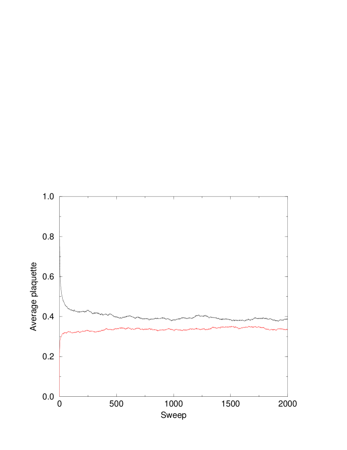
Figure 4: Metastability on the $16^{3}\times 8$ lattices for $\beta_{V}=2.4$, $\beta_{F}=1.1852$. This is near, but not necessarily right on top of, the first order transition.

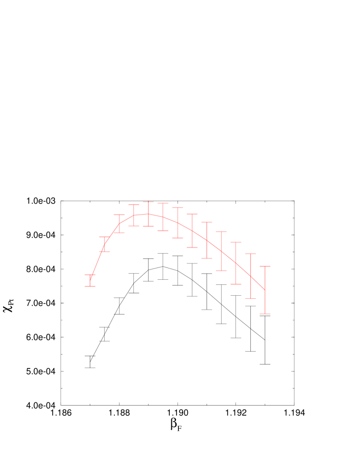
Figure 5: Peak in the temporal Polyakov loop susceptibility $\chi_{P_{t}}$ on the $16^{3}\times 8$ (upper) and $18^{3}\times 8$ lattices at $\beta_{V}=2.4$.

These results strongly suggest it would be worthwhile to do a higher statistics run on a larger lattice in this region. We have therefore simulated $16^{3}\times 8$ and $18^{3}\times 8$ lattices at $\beta_{V}=2.4$ just to the right of the first order effects. The latter can clearly be seen in figure 4; this may not be exactly at the phase transition, due to the difficulties locating it on a lattice of this size, but is close to it. However, we can still pick out a separate peak in the $\chi_{P_{t}}$ susceptibility at $\beta_{F}=1.190(2)$, shown in figure 5, where our simulations show no sign of metastability and are indeed all on the high-$\beta_{F}$ side of the first order transition. The range of reweighting in the figure is limited to that which statistics seem to allow: at least 1% of the data corresponds to an average action whose $\beta_{F}$ is more remote from the simulated value than the reweighting point. From table 2, the ratio of susceptibilities of equation 9 is $1.20(7)$, compared with the expectation 1.15 for a second order and 1.42 for a first order transition. This confirms that the transition is second order.

We consequently feel entitled to claim that the second order, finite temperature effects separate out from the first order, bulk effects near the lower end of the latter for time sizes $N_{T}\gtrsim 8$, and that this is the resolution of the universality problem.

Why should we see the apparent finite temperature effects, if the transition is really bulk? The following point may be relevant: there is an interesting parallel between these effects and those seen in a version of the compact lattice U(1) gauge theory, where one forms a similarly modified action,

$$S=-\sum_{\Box}(\beta\cos\theta_{\Box}+\gamma\cos 2\theta_{\Box})$$ (11)

where $\theta_{\Box}$ is the plaquette angle [17]. Here again, there is a phase transition — although definitely bulk in the U(1) theory — which was found to change from second to first order as the coupling with the extra symmetry, here $\gamma$, was increased. In reference [16], an investigation was made of this region, and the tricritical point where the behaviour changed located. Our point is that near the tricritical region significant finite size effects were seen, even on lattices of size $12^{4}$ and $14^{4}$. Applied to table 3, this fits in with our interpretation of the results.

4 Mixing of first and second order effects

The evidence is that the finite temperature and the bulk transition do separate out for sufficiently large lattices. If one is interested only in universality, and is prepared to dismiss the bulk effects as an uninteresting lattice artefact, one can stop worrying at this point. We, however, shall discuss the nature of this further.

Heller has found[20] for the corresponding fundamental/adjoint plane in SU(3) that there is also a clear separation between the bulk effects and the deconfinement transition, but that it occurs for rather smaller lattices; it seems that in this case the bulk effects are not so strong. Possibly the difference lies in topology of the gauge manifold. Problems in the continuum limit of certain gauge groups with a non-trivial topology like that of the SO(3) case here have been raised [21]. The behaviour in the representations of SU(3) has not yet been addressed, but it may be that the effects there are sufficiently different to explain the distinct results.

In explaining the mixing of the effects for lattices with $N_{T}\lesssim 8$, it is perhaps easiest to think of a more basic picture of first order transitions, with no specifically field-theoretic features. The idea of physics being ‘hidden’, as our second order transition apparently is by the bulk effects, is quite familiar from elementary thermodynamics. Consider the water/steam transition: metastability here is the property that allows one to trace at least partly the hidden parts of the surface, as in superheating or supercooling; a critical end point represents the straightening out of the surface so that no such features occur.

We suggest thinking of the known bulk transitions in the SU(2)/SO(3) model in a similar way. For example, in increasing $\beta_{V}$ from one side of the Z(2) monopole transition to the other, we are passing from one range of physics in the gauge theory to another. Without this first order effect, the gauge dynamics would vary smoothly from strong to weak coupling, so we are skipping over some inaccessible region — which quite likely includes, for example, whatever finite temperature crossover is taking place in SO(3).

Presumably the conjunction of the two separate bulk transitions makes this more complicated. It would not be surprising if it had long range effects; indeed, it has been suggested for a long time that the famous peak in the specific heat of the plaquette of SU(2) — equivalently, the sharp crossover in the average action — is a long-range remnant of what was then thought to be a bulk end point. This is reinforced by figure 2: it is clear that even where the deconfinement transition is visible as a second order line, the lines for $N_{T}=2$ and 4 are converging, contrary to the naive expectation that they are parallel at some effective beta given by equation 4.

Figure 6: Freehand sketch of the presumed behaviour of the action in the crossover region of the average action below (full), at (dashed) and above (dotted) the end point of the first order transition. The instability in the last case causes the discontinuous behaviour.

Figure 6 shows what we presume to be the behaviour of the action below, on, and above the first order endpoint. In the third case (dotted line), the second order transition (along, of course, with all other physics in the range of couplings) is hidden on what one may think of as the ‘superheated’ and ‘supercooled’ branches of the line, which are not seen because the instability in the action causes it to flip from the high to the low side. The tricritical point (dashed line) is like the end point of the water/steam phase transition in that the hidden regions disappear and the crossover from one phase to another becomes smooth. Our case is more complicated because part of this smooth physics is the physical second order transition.

This agrees with the observation that the first order transition becomes stronger with increasing $\beta_{V}$ and that the discontinuity in the average plaquette increases (as shown by our tricritical fit above). The dependence on the temporal extent of the lattice indicates the sensitivity to the changes taking place, which may not be finite temperature effects. Then the deconfining transition itself is invisible in the $(\beta_{F},\beta_{V})$ plane for sufficiently small $N_{T}$.

The conclusions are supported by the other calculations of the monopole $\langle M\rangle$ and charge $\langle E\rangle$, defined in equation 5 and their effective values deduced from the plaquette $\langle\bar{M}\rangle$ and $\langle\bar{E}\rangle$ defined in equation 6. The behaviour of these is as given in reference [9]; they too are discontinuous at the first order lines, but show in any case a fairly sharp crossover from near 1 at low $\beta_{F}$ to near 0 at high values. We have nothing to add in detail to the picture shown in figure 5 of reference [9], which shows a larger range of $\beta_{F}$ (there called $\delta$) than we have used. The region where this occurs appears to be the same as where the plaquette action shows a steep change. We consider this to be evidence in favour of the traditional picture of the first order effects: that they are an instability caused by the increasingly sharp crossover in the action.

Extended action

We supplement our evidence from the $12^{4}$ lattices, that the bulk and finite temperature transitions can be seen separately at least at $\beta_{V}=2.4$, with the following.

Given our contention that the first order effects do not represent continuum physics, one might wonder whether an improved action such as Symanzik’s tree-level improved action [18] would change the picture, in that one is brought closer to the continuum for a given lattice size by explicitly eliminating terms in the expansion of the lattice action up to the next even power of $a$, $\mathcal{O}(a^{6})$. The action with this first order improvement is defined by:

$$S_{Fi}=-\frac{\beta_{Fi}}{2}\left(\frac{5}{3}\sum_{\Box}\operatorname{Tr}_{F}U_{\Box}-\frac{1}{2}\sum_{[1\times 2]}\operatorname{Tr}_{F}U_{[1\times 2]}\right)$$ (12)

in which the usual plaquette term has been supplemented by a sum over all rotations of all $1\times 2$ rectangles on the lattice and we use the subscript $Fi$ to denote an improvement in the fundamental part of the action. Such actions have been shown to have problems when looking at properties derived from two-point functions, presumably related to their lack of positivity [19]; also, we do not know if the perturbative coefficients are close to the optimum for non-perturbative simulations. However, there should be no problem in simply looking for some sort of improvement in a phase transition with a naive perturbative improvement.

Figure 7: Metastability for the unimproved $8^{3}\times 4$ lattice with $\beta_{F}=1.181$, $\beta_{V}=2.4$, showing the average Polyakov loop in the finite temperature direction.

We have simulated using the action in equation 12 for the fundamental coupling only. This will allow us to use the unchanged $\beta_{V}$ axis as a yardstick for how well the improved action is performing. We again pick $N_{T}=4$ for $N_{S}=8$ and 10 at $\beta_{V}=2.4$. To demonstrate that in the unimproved case there is metastability suggestive of a first order transition, we show the behaviour of the temporal Polyakov loop on a lattice of the same size at $\beta_{F}=1.181$ in figure 7: it is clear there is a two state signal, with one phase confined, the other deconfined.

With the improved action we find no sign of first order effects. We instead find a smooth change of behaviour with a peak in $\chi_{P_{t}}$ at $\beta_{Fi}=0.827(2)$; the scaling behaviour clearly suggests a second order nature (table 2). (Note that there is a rescaling of $\beta_{F}$ in the improved case; this is not important so long as we can identify the corresponding physical regions.)

There is thus a clear — in fact, a qualitative — difference of behaviour between the unimproved and improved action at the same $\beta_{V}$. As we are using the same Villain part of the action, we can be sure the difference is due to the improvement in the fundamental part. We hold this to be evidence for our contention that the first order effects are artefacts irrelevant to the continuum limit of the gauge theory. There may still be some continuum limit at the end of the first order transition, but we suggest it is not simply related to that of the usual SU(2) theory.

We have also simulated at $\beta_{V}=2.5$: here the improved action too shows the two state behaviour, with a transition in the vicinity of $\beta_{Fi}\sim 0.79$, so (as one would expect) the effect of the first-order improvement is fairly small.

5 Conclusions

We have attempted to resolve the confusions found in pure SU(2) lattice gauge theory with a mixed fundamental/SO(3) action. We have used the Halliday–Schwimmer action which allows efficient updating. Our conclusions are summarised in figure 2, where for clarity the data points are not shown and should be read off from tables 1 to 3, and in an expansion of the area around the endpoint of the first order behaviour in figure 3.

We confirm that for lattices with small extension $N_{T}$ the finite temperature SU(2) transition runs into a region where first order effects dominate.

On small lattices, between $N_{T}=2$ and $4$ sites in the finite temperature direction, we see a shift in the position of the first order effects to higher fundamental inverse coupling $\beta_{F}$, as seen by references [1, 2, 3]. For larger $N_{T}$, and at slightly increased SO(3) coupling $\beta_{V}$, this effect decreases and we suggest it is due to large finite size (in the sense that they disappear on larger lattices) rather than temperature effects. This supports the traditional view that the first order effects have a bulk nature and are unrelated to the true finite temperature transition.

We have reinforced the suggestion that the first order effects are not related to the continuum limit of SU(2) by showing that they are shifted to larger $\beta_{V}$ by the use of an order-$a$ improved gauge action.

The evidence we have presented suggests that the finite temperature transition will separate out from the bulk effects, and has indeed started to do so at the lower end of the bulk effects, around $\beta_{V}=2.4$, for $N_{T}=8$. In this case (in contrast to SU(3)) the process is likely to be gradual: at $\beta_{V}=3.0$, for example, the $12^{4}$ lattice again shows Polyakov loop symmetry breaking across the first order transition, showing that the finite temperature effects have been reabsorbed into the bulk ones. There is therefore no reason to doubt that eventually the former will emerge cleanly from the latter for a lattice with a sufficiently large temporal extent. Clearly, this would require huge lattices and statistics to sort out quantitatively; eventually one has to worry about the intersection with the Z(2) symmetry breaking transition at large $\beta_{V}$. This is probably out of reach at the moment.

Nonetheless, we suggest that the problems of universality in this theory are essentially resolved, and that the true finite temperature transition in the extended SU(2) plain remains second order, while the first order effects present are bulk artefacts which are modified by small lattice dimensions.

While this work was being finalised, a new preprint appeared further disputing the nature of the first order line in the region containing the endpoint, based on a finite size scaling analysis [22]. To resolve this would involve a more detailed investigation of the tricritical region.

References

- [1] Rajiv V. Gavai, Michael Grady and Manu Mathur, Nucl. Phys. B423 (1994) 123.
- [2] Manu Mathur and Rajiv V. Gavai, Nucl. Phys. B448 (1995) 399.
- [3] Rajiv V. Gavai and Manu Mathur, ‘On the order of the SU(2) deconfinement transition’, hep-lat/9512015.
- [4] M. Creutz, ‘Quarks, gluons and lattices’, Cambridge University Press, Cambridge, 1983, chapter 20.
- [5] P.W. Stephenson, “New results from mixed action lattice gauge theory”, to be published in the proceedings of the EPS-HEP conference, Brussels, July 1995, hep-lat/9509070.
- [6] I.G. Halliday and A. Schwimmer, Phys. Lett. 101B (1981) 327.
- [7] I.G. Halliday and A. Schwimmer, Phys. Lett. 102B (1981) 337.
- [8] Gyan Bhanot and Michael Creutz, Phys. Rev. D24 (1981) 3212.
- [9] L. Caneschi, I.G. Halliday and A. Schwimmer, Nucl. Phys. B200[FS4] (1982) 409.
- [10] J. Engels, J. Fingberg and M. Weber, Nucl. Phys. B332 (1990) 737
- [11] J. Engels, J. Fingberg and D.E. Miller, Nucl. Phys. B387 (1992) 501
- [12] J. Fingberg, U. Heller and F. Karsch, Nucl. Phys. B392 (1993) 493.
- [13] Poul H. Damgaard, Jeff Greensite and Martin Hasenbusch, ‘Deconfinement, Screening and Abelian Projection at Finite Temperature’, NBI-HE-95-35, hep-lat/9511007.
- [14] A.D. Kennedy and B.J. Pendleton, Phys. Lett. 156B (1985) 393.
- [15] A.M. Ferrenberg and R.H. Swendsen, Phys. Rev. Lett. 61 (1988) 2635
- [16] H.G. Evertz, T. Jersák, T. Neuhaus and P.M. Zerwas, Nucl. Phys. B251 [FS13] (1985) 279.
- [17] G. Bhanot, Nucl. Phys. B205[FS5] (1982) 168.
- [18] K. Symanzik, Nucl. Phys. B226 (1983) 187;Nucl. Phys. B226 (1983) 205.
- [19] C. Michael and M. Teper, Nucl. Phys. B305 [FS23] (1988) 453.
- [20] Urs M. Heller, Phys. Lett. B362 (1995) 123;“More on SU(3) lattice gauge theory in the fundamental adjoint plane”, Urs M. Heller, to appear in Proceedings of Lattice’95, FSU preprint FSU-SCRI-95C-85, hep-lat/9509010
- [21] M. Hasenbusch and R.R. Horgan, ‘Tests of the continuum limit for the SO(4) Principal Chiral Model and the prediction for , Cambridge preprint DAMTP-95-62, hep-lat/9511004.
- [22] Rajiv V. Gavai, ‘A study of the bulk phase transition of the SU(2) lattice gauge theory with mixed action’, Minnesota preprint TPI-MINN-96/03, hep-lat/9603003.