Massive Fermions in Lattice Gauge Theory

Aida X. El-Khadra,a Andreas S. Kronfeld,b and Paul B. Mackenzieb
aPhysics Department, University of Illinois,
1110 W. Green Street, Urbana, IL 61801
bTheoretical Physics Group, Fermi National Accelerator Laboratory,
P.O. Box 500, Batavia, IL 60510
(4 April 1996)
Abstract

This paper presents a formulation of lattice fermions applicable to all quark masses, large and small. We incorporate interactions from previous light-fermion and heavy-fermion methods, and thus ensure a smooth connection to these limiting cases. The couplings in improved actions are evaluated for arbitrary fermion massย mqsubscript๐‘š๐‘žm_{q}, without expansions around small- or large-mass limits. We treat both the action and external currents. By interpreting on-shell improvement criteria through the lattice theoryโ€™s Hamiltonian, one finds that cutoff artifacts factorize into the form bnโ€‹(mqโ€‹a)โ€‹[๐’‘โ€‹a]snsubscript๐‘๐‘›subscript๐‘š๐‘ž๐‘Žsuperscriptdelimited-[]๐’‘๐‘Žsubscript๐‘ ๐‘›b_{n}(m_{q}a)[\mbox{\boldmath$p$}a]^{s_{n}}, where ๐’‘๐’‘p is a momentum characteristic of the system under study, snsubscript๐‘ ๐‘›s_{n} is related to the dimension of the n๐‘›nth interaction, and bnโ€‹(mqโ€‹a)subscript๐‘๐‘›subscript๐‘š๐‘ž๐‘Žb_{n}(m_{q}a) is a bounded function, numerically alwaysย Oโ€‹(1)O1{\rm O}(1) or less. In heavy-quark systems ๐’‘๐’‘p is typically rather smaller than the fermion massย mqsubscript๐‘š๐‘žm_{q}. Therefore, artifacts of order (mqโ€‹a)ssuperscriptsubscript๐‘š๐‘ž๐‘Ž๐‘ (m_{q}a)^{s} do not arise, even when mqโ€‹aโ€‹โˆผ>1subscript๐‘š๐‘ž๐‘Žโˆผ>1m_{q}a\mathop{\raisebox{-1.72218pt}{\hbox to0.0pt{$\sim$\hss}}\raisebox{1.72218pt}{$>$}}1. An important by-product of our analysis is an interpretation of the Wilson and Sheikholeslami-Wohlert actions applied to nonrelativistic fermions.

1 Introduction

The most promising avenue for a quantitative understanding of nonperturbative quantum chromodynamicsโ€”and other field theoriesโ€”is via numerical (Monte Carlo) integration of functional integrals defined on a latticeย [1]. Like any numerical technique this method has uncertainties that must be understood and controlled before the results are useful. In particular, although the continuum theory is defined by the limit of a sequence of lattice theories, the numerical calculations are never carried out at the limit. Because the Monte Carlo introduces statistical errors, the extrapolation to the continuum limit is imperfect. The results for physical quantities are consequently contaminated by lattice artifacts. For a practical result, this uncertainty must be smaller than, say, relevant experimental uncertainties.

The way to reduce lattice artifacts is based on the renormalization groupย [2]. One starts with a general action

$$S=\sum_{n}c_{n}S_{n},$$ (1.1)

where theย Snsubscript๐‘†๐‘›S_{n} include all interactions with the desired field content and the appropriate symmetries. One approach to the continuum limit, which might be called brute force, is to choose theย cnsubscript๐‘๐‘›c_{n} in any way that drives the lattice spacing to zero. An ideal approach would be to choose theย cnsubscript๐‘๐‘›c_{n} to lie on a renormalized trajectoryย [2], where there are no lattice artifacts even though the lattice spacingย aโ‰ 0๐‘Ž0{a\neq 0}. In the space of all possible actions specified by eq.ย (1.1), the renormalized trajectories lie in a subspace, whose dimension equals the number of relevant parameters. Once the relevant parameters have been fixed by physics, they and the renormalization scheme determine all theย cnsubscript๐‘๐‘›c_{n}.

Unfortunately, a renormalized trajectory is mostly of abstract value, because on one infinitely manyย cnsubscript๐‘๐‘›c_{n} are nonzero. All practical schemes, such as blocking fieldsย [3] or Symanzik improvementย [4] use criteria such as localityย [3] or the scaling dimensionย [4] to truncate the space of actions. (For an asymptotically free theory, such as QCD, these two criteria are not very different.) Furthermore, the calculations of theย cnsubscript๐‘๐‘›c_{n} are, in practice, only approximate. For these reasons an improved action is only partially renormalized. Nevertheless, any practical action can be written

$$S={\cal S}_{\rm RT}-\delta S,$$ (1.2)

where ${\cal S}_{\rm RT}$ denotes (an action on) the renormalized trajectory. Usually the truncations and/or approximations used to generateย S๐‘†S will also yield estimates for the remaining cutoff effectsย ฮดโ€‹S๐›ฟ๐‘†\delta S.

This paper treats massive fermions coupled to non-Abelian gauge fields. The relevant couplings are the fermion masses and the gauge coupling. So the renormalized trajectory takes the form

$${\cal S}_{\rm RT}(m_{q}/\Lambda_{\rm QCD},\Lambda_{\rm QCD}a)=\sum_{n}c_{n}(m_{0}a,g_{0}^{2})S_{n},$$ (1.3)

where $m_{q}$ denotes the fermion mass,111We use $m_{q}$ for a quark mass defined by a physical condition andย m0โ€‹asubscript๐‘š0๐‘Žm_{0}a for the coupling appearing in the action. $\Lambda_{\rm QCD}$ is the scale characteristic of the gauge theory, and the argument $\Lambda_{\rm QCD}a$ labels the renormalization point. Theย Snsubscript๐‘†๐‘›S_{n} are gauge-invariant combinations of four-component fermion and anti-fermion fields ($\psi$ and $\bar{\psi}$) and the lattice gauge fieldย ($U_{\mu}$). For later calculational convenience we choose the bare, rather than some physical, fermion massย m0โ€‹asubscript๐‘š0๐‘Žm_{0}a and gauge couplingย g02superscriptsubscript๐‘”02g_{0}^{2} to parameterize the couplingsย cnsubscript๐‘๐‘›c_{n}.

As $a\to 0$ the fermion mass $m_{q}a$ is formally smaller thanย g02superscriptsubscript๐‘”02g_{0}^{2}. (By asymptotic freedom $g_{0}^{2}=[\beta_{0}\log(\Lambda_{\rm QCD}^{2}a^{2})]^{-1}$ asย aโ†’0โ†’๐‘Ž0a\to 0.) It is therefore tempting to expand the couplings $c_{n}(m_{0}a,g_{0}^{2})$ inย m0โ€‹asubscript๐‘š0๐‘Žm_{0}a, as in previous analysesย [5, 6, 7]. But there may be fermions satisfying $m_{q}/\Lambda_{\rm QCD}\gg 1$; the charm, bottom, and top quarks are examples in nature. If, in practice, $m_{q}a$ is not small, perturbation theory inย m0โ€‹asubscript๐‘š0๐‘Žm_{0}a need not be useful, even though perturbation theory inย g02superscriptsubscript๐‘”02g_{0}^{2} might be. Indeed, this regime includes the charm and bottom quarks at currently accessible lattice spacings.

The staticย [8, 9] and nonrelativisticย [10, 11, 12] effective theories address the problems of heavy fermions. Their restriction to $m_{q}\gg\Lambda_{\rm QCD}$ implies that couplings of interactions between particle and antiparticle states may be chosen to vanish, and the remaining interactions in eq.ย (1.1) are organized according to a $\mbox{\boldmath$p$}/m_{q}$ expansion. But for some $m_{q}\sim 2\Lambda_{\rm QCD}$ the expansion is no longer useful. Furthermore, radiative corrections induce power-law terms, e.g.ย g02/(mqโ€‹a)superscriptsubscript๐‘”02subscript๐‘š๐‘ž๐‘Žg_{0}^{2}/(m_{q}a), which must be canceled by adjusting theย cnsubscript๐‘๐‘›c_{n}. These terms, which diverge as $a\to 0$, are a reminder that the effective theories are to be used at scales below (large)ย mqsubscript๐‘š๐‘žm_{q}. Their presence implies that cutoff effects in the effective theories should be removed not by brute force, but by keeping $a\sim m_{q}^{-1}$ and constructing actions systematically closer to the renormalized trajectoryย [11, 12].

This paper presents a way to encompass both the small and large mass formulations. The doubling problem is handled by Wilsonโ€™s methodย [13]. In addition to treating the m0โ€‹asubscript๐‘š0๐‘Žm_{0}a dependence of the couplings exactly, the central idea is to enlarge the class of interactions considered in eq.ย (1.3) to include those from both the smallย m0โ€‹asubscript๐‘š0๐‘Žm_{0}a and the largeย mq/ฮ›QCDsubscript๐‘š๐‘žsubscriptฮ›QCDm_{q}/\Lambda_{\rm QCD} limits. In particular, we do not impose a symmetry between couplings of interactions that would be related by interchanging the time axis with a spatial axis. For any mqโ€‹asubscript๐‘š๐‘ž๐‘Žm_{q}a, the four-momentum of a quark in most interesting physical systems satisfies [Eโ€‹(๐’‘)โˆ’Eโ€‹(๐ŸŽ)]โ€‹aโ‰ช1much-less-thandelimited-[]๐ธ๐’‘๐ธ0๐‘Ž1[E(\mbox{\boldmath$p$})-E({\bf 0})]a\ll 1 wheneverย ๐’‘โ€‹aโ‰ช1much-less-than๐’‘๐‘Ž1\mbox{\boldmath$p$}a\ll 1. But when mqโ€‹a>1subscript๐‘š๐‘ž๐‘Ž1m_{q}a>1 the characteristic four-momentum of the physics does not respect time-space axis interchange. Under such circumstances it is inconvenient and unnecessary to choose an axis-interchange symmetric action.222Relinquishing axis-interchange symmetry is common in treatments of heavy quarks with momentum-space and dimensional regulators. It is possible to derive deviations from heavy-quark symmetry from the Dirac actionย [14, 15], while maintaining time-space axis interchange invariance as a corollary to Euclidean invariance. But usually the derivations are easier with a nonrelativistic actionย [10, 16], the so-called the heavy-quark effective theoryย [17].

In the appropriate limits, our formulation of lattice fermions shares properties of previous ones. On one hand, at dimension five or less, couplings related by axis interchange become identical in the limit m0โ€‹aโ†’0โ†’subscript๐‘š0๐‘Ž0m_{0}a\to 0: the Wilson action and the improved action of ref.ย [6] are recovered. But when m0โ€‹aโ‰ 0subscript๐‘š0๐‘Ž0m_{0}a\neq 0 the mass-dependent renormalization leaves lattice artifacts that are proportional toย ๐’‘โ€‹a๐’‘๐‘Ž\mbox{\boldmath$p$}a andย ฮ›QCDโ€‹asubscriptฮ›QCD๐‘Ž\Lambda_{\rm QCD}a, notย mqโ€‹asubscript๐‘š๐‘ž๐‘Žm_{q}a. At higher dimension, however, we retain Wilsonโ€™s time derivative and incorporate โ€œspatial-onlyโ€ interactions into eq.ย (1.1).

On the other hand, for ${m_{q}\gg\Lambda_{\rm QCD}}$ one can interpret the lattice theory in a nonrelativistic light. Indeed, all members of our class of actions approach a universal static limit asย m0โ€‹aโ†’โˆžโ†’subscript๐‘š0๐‘Žm_{0}a\to\infty. For $m_{0}a$ large but finite, the 1/mqs1superscriptsubscript๐‘š๐‘ž๐‘ 1/m_{q}^{s} corrections to the static limit can be recovered systematically, provided the fermion mass is defined through the kinetic energy, and provided the general action, eq.ย (1.3), is truncated only at dimensionย 4+s4๐‘ 4+s (or higher). Unlike previous implementations of nonrelativistic fermions, however, our approach crosses smoothly over into the regime of tiny lattice spacings, whereย m0โ€‹aโ‰ช1much-less-thansubscript๐‘š0๐‘Ž1m_{0}a\ll 1 even for a heavy quark. Thus, after severalย cnsubscript๐‘๐‘›c_{n} have been tuned close to a renormalized trajectory, thereby removing the worst lattice artifacts, a little brute force can remove theย rest.

Because we make no assumptions about the ratio of fermion masses to other scales, our formulation is especially well suited to fermions too heavy for small $m_{0}a$ methods yet too light for large $m_{q}/\Lambda_{\rm QCD}$ methods. With the actions given below one can test whether a given fermion is heavy enough to be treated nonrelativistically, without resorting to brute-force simulations. Aย practical example might be the charm quark, which has a mass only a few times $\Lambda_{\rm QCD}$, yet even on the finest lattices available today $m_{\rm ch}a$ is largish, at leastย 1313\frac{1}{3}.

For a concrete determination of the $c_{n}$, one must choose a renormalization group, a criterion for truncating the sum in eq.ย (1.3), and a strategy for determining theย cnsubscript๐‘๐‘›c_{n}. For illustration we adopt here a Symanzik-like procedureย [4], organizing the interactions by dimension. Carrying out this program to arbitrarily high dimension would produce a renormalized trajectory of a renormalization group generated by infinitesimal changes inย a๐‘Ža. For simplicity, however, most of this paper treats interactions only up to dimension five. Although a nonperturbative determination of the couplings is possible in principle, this paper makes the further approximation of perturbation theory in $g_{0}^{2}$, that is

$$c_{n}(m_{0}a,g_{0}^{2})=\sum_{l=0}^{\infty}g_{0}^{2l}c_{n}^{[l]}(m_{0}a).$$ (1.4)

Except for sect.ย 8 we work to tree level, so we often abbreviate $c_{n}^{[0]}(m_{0}a)$ by $c_{n}(m_{0}a)$. (Explicit one-loop calculations are in progressย [18].) Within these approximations we determine theย cnsubscript๐‘๐‘›c_{n} by insisting that on-shell quantities take their desired values, as first suggested by Lรผscher and Weiszย [19].

One calculational procedure is to work out n๐‘›n-point on-shell Green functions via Feynman diagrams and tune them to the continuum limit, to the appropriate order inย ๐’‘๐’‘p. An example is in sect.ย 4. Because this strategy is limited to a finite number of quantities, it is nontrivial to assume that other quantities are improved tooย [4]. An alternative is developed in sect.ย 5. Starting from the transfer matrix we derive an expression for the fermion Hamiltonian, valid (at tree level) for states withย ๐’‘โ€‹aโ‰ช1much-less-than๐’‘๐‘Ž1\mbox{\boldmath$p$}a\ll 1. Because the Hamiltonian is an operator, improving it to some accuracy guarantees the improvement to the same accuracy of infinitely many c๐‘c-numbers. We show that by adjusting the couplings cnโ€‹(m0โ€‹a)subscript๐‘๐‘›subscript๐‘š0๐‘Žc_{n}(m_{0}a) correctly, and allowing physically unobservable redefinitions of the fermion field, one can tune the Hamiltonian to the continuum limit, i.e.ย to the Dirac Hamiltonian, to the appropriate order inย ๐’‘๐’‘p.

In addition to equations for the $c_{n}$, the analysis of the Hamiltonian yields two important results. One is that the Wilson time derivative needs no improvement. The other is a canonically normalized fermion field that, to the accuracy of the improvement, obeys Diracโ€™s (continuum) equation of motion. This field is a potent ingredient in calculations of matrix elements involving heavy-quark systems; see sect.ย 7.

Owing to the approximations introducedโ€”the truncation of interactions and perturbation theoryโ€”some cutoff effects remain. If these errors are small, they may be estimated by insertions of $\delta S$ in correlation functions. If the series for $c_{n}(m_{0}a,g_{0}^{2})$ has been developed to $L_{n}$-th order

$$\delta S=\sum_{n}\,\sum_{l=L_{n}+1}^{\infty}g_{0}^{2l}c_{n}^{[l]}(m_{0}a)S_{n}.$$ (1.5)

Aย typical term in ฮดโ€‹S๐›ฟ๐‘†\delta S distorts an on-shell correlation function by an amount of order g02โ€‹lโ€‹cn[l]โ€‹(m0โ€‹a)โ€‹(๐’‘โ€‹a)snsuperscriptsubscript๐‘”02๐‘™superscriptsubscript๐‘๐‘›delimited-[]๐‘™subscript๐‘š0๐‘Žsuperscript๐’‘๐‘Žsubscript๐‘ ๐‘›g_{0}^{2l}c_{n}^{[l]}(m_{0}a)(\mbox{\boldmath$p$}a)^{s_{n}}, where sn=dimSnโˆ’4subscript๐‘ ๐‘›dimensionsubscript๐‘†๐‘›4{s_{n}}=\dim S_{n}-4, andย lโ‰ฅLn+1๐‘™subscript๐ฟ๐‘›1l\geq L_{n}+1. (If Snsubscript๐‘†๐‘›S_{n} is omitted from the action altogether, then here l=0๐‘™0l=0.) The analysis presented below shows that the tree-level, lower-dimension cn[0]โ€‹(m0โ€‹a)superscriptsubscript๐‘๐‘›delimited-[]0subscript๐‘š0๐‘Žc_{n}^{[0]}(m_{0}a) are well-behaved for all masses. We also show that loop diagrams have the same or more benign behavior at large mass. In particular, as m0โ€‹aโ†’โˆžโ†’subscript๐‘š0๐‘Žm_{0}a\to\infty the cn[l]โ€‹(m0โ€‹a)superscriptsubscript๐‘๐‘›delimited-[]๐‘™subscript๐‘š0๐‘Žc_{n}^{[l]}(m_{0}a) either approach a constant or fall asย (mqโ€‹a)โˆ’ssuperscriptsubscript๐‘š๐‘ž๐‘Ž๐‘ (m_{q}a)^{-s}, for some sโ‰คsn๐‘ subscript๐‘ ๐‘›s\leq s_{n}. These results provide evidence that the higher-dimensionย cnโ€‹(m0โ€‹a)subscript๐‘๐‘›subscript๐‘š0๐‘Žc_{n}(m_{0}a) are well-behaved too.

In Monte Carlo programs it is customary to parameterize the action by the hopping parameter instead of the mass. In this notation the dimension-three and -four interactions are written

S0=โˆ‘nฯˆยฏnโ€‹ฯˆnโˆ’ฮบtโ€‹โˆ‘n[โ€‹ฯˆยฏnโ€‹(1โˆ’ฮณ0)โ€‹Un,0โ€‹ฯˆn+0^+ฯˆยฏn+0^โ€‹(1+ฮณ0)โ€‹Un,0โ€ โ€‹ฯˆn]โˆ’ฮบsโ€‹โˆ‘n,i[โ€‹ฯˆยฏnโ€‹(rsโˆ’ฮณi)โ€‹Un,iโ€‹ฯˆn+ฤฑ^+ฯˆยฏn+ฤฑ^โ€‹(rs+ฮณi)โ€‹Un,iโ€ โ€‹ฯˆn].subscript๐‘†0subscript๐‘›subscriptยฏ๐œ“๐‘›subscript๐œ“๐‘›subscript๐œ…๐‘กsubscript๐‘›delimited-[]subscriptยฏ๐œ“๐‘›1subscript๐›พ0subscript๐‘ˆ๐‘›0subscript๐œ“๐‘›^0subscriptยฏ๐œ“๐‘›^01subscript๐›พ0subscriptsuperscript๐‘ˆโ€ ๐‘›0subscript๐œ“๐‘›subscript๐œ…๐‘ subscript๐‘›๐‘–delimited-[]subscriptยฏ๐œ“๐‘›subscript๐‘Ÿ๐‘ subscript๐›พ๐‘–subscript๐‘ˆ๐‘›๐‘–subscript๐œ“๐‘›^italic-ฤฑsubscriptยฏ๐œ“๐‘›^italic-ฤฑsubscript๐‘Ÿ๐‘ subscript๐›พ๐‘–superscriptsubscript๐‘ˆ๐‘›๐‘–โ€ subscript๐œ“๐‘›\begin{array}[]{l}S_{0}={\displaystyle\sum_{n}}\bar{\psi}_{n}\psi_{n}-\kappa_{t}{\displaystyle\sum_{n}}\left[\rule{0.0pt}{9.70001pt}\bar{\psi}_{n}(1-\gamma_{0})U_{n,0}\psi_{n+\hat{0}}+\bar{\psi}_{n+\hat{0}}(1+\gamma_{0})U^{\dagger}_{n,0}\psi_{n}\right]\\[10.00002pt] \hskip 63.00012pt-\,\kappa_{s}{\displaystyle\sum_{n,i}}\left[\rule{0.0pt}{9.70001pt}\bar{\psi}_{n}(r_{s}-\gamma_{i})U_{n,i}\psi_{n+\hat{\imath}}+\bar{\psi}_{n+\hat{\imath}}(r_{s}+\gamma_{i})U_{n,i}^{\dagger}\psi_{n}\right].\end{array} (1.6)

Some terms of dimension fiveโ€”to solve the doubling problemย [13]โ€”are included here too. The relation between the bare massย m0โ€‹asubscript๐‘š0๐‘Žm_{0}a and the hopping parameters $\kappa_{t}$ and ฮบssubscript๐œ…๐‘ \kappa_{s} is given below in sect.ย 2. Eq.ย (1.6) illustrates how our program subsumes properties of the familiar small-mass and large-mass formulations. Imposing axis-interchange invariance would set ฮบs=ฮบtsubscript๐œ…๐‘ subscript๐œ…๐‘ก\kappa_{s}=\kappa_{t} and rs=1subscript๐‘Ÿ๐‘ 1r_{s}=1, and then $S_{0}$ reduces to the Wilson actionย [13]. Rewriting rsโ€‹ฮบs=cssubscript๐‘Ÿ๐‘ subscript๐œ…๐‘ subscript๐‘๐‘ r_{s}\kappa_{s}=c_{s} and setting ฮบssubscript๐œ…๐‘ \kappa_{s} to zero with csโ‰ 0subscript๐‘๐‘ 0c_{s}\neq 0 produces the simplest nonrelativistic actionย [11].

This pattern continues for dimension-five interactions. Aside from the Wilson terms inย S0subscript๐‘†0S_{0}, the other dimension-five interactions are the chromomagnetic interaction

SB=i2โ€‹cBโ€‹ฮบsโ€‹โˆ‘n;i,j,kฮตiโ€‹jโ€‹kโ€‹ฯˆยฏnโ€‹ฯƒiโ€‹jโ€‹Bn;kโ€‹ฯˆn,subscript๐‘†๐ต๐‘–2subscript๐‘๐ตsubscript๐œ…๐‘ subscript๐‘›๐‘–๐‘—๐‘˜subscript๐œ€๐‘–๐‘—๐‘˜subscriptยฏ๐œ“๐‘›subscript๐œŽ๐‘–๐‘—subscript๐ต๐‘›๐‘˜subscript๐œ“๐‘›S_{B}=\mbox{\small$\frac{i}{2}$}c_{B}\kappa_{s}\sum_{n;i,j,k}\varepsilon_{ijk}\bar{\psi}_{n}\sigma_{ij}B_{n;k}\psi_{n}, (1.7)

and the chromoelectric interaction

SE=iโ€‹cEโ€‹ฮบsโ€‹โˆ‘n;iฯˆยฏnโ€‹ฯƒ0โ€‹iโ€‹En;iโ€‹ฯˆn,subscript๐‘†๐ธ๐‘–subscript๐‘๐ธsubscript๐œ…๐‘ subscript๐‘›๐‘–subscriptยฏ๐œ“๐‘›subscript๐œŽ0๐‘–subscript๐ธ๐‘›๐‘–subscript๐œ“๐‘›S_{E}=ic_{E}\kappa_{s}\sum_{n;i}\bar{\psi}_{n}\sigma_{0i}E_{n;i}\psi_{n}, (1.8)

whereย B๐ตB andย E๐ธE are suitable functions of the lattice gauge fieldย U๐‘ˆU, as in sect.ย 2. The light-quark formalism of refs.ย [6, 7] considers the special case $c_{B}=c_{E}$, whereas the heavy-quark formalism of refs.ย [11, 12] setsย cE=0subscript๐‘๐ธ0c_{E}=0.

The couplingsย rssubscript๐‘Ÿ๐‘ r_{s}, ฮถ=ฮบs/ฮบt๐œsubscript๐œ…๐‘ subscript๐œ…๐‘ก\zeta=\kappa_{s}/\kappa_{t}, $c_{B}$, andย cEsubscript๐‘๐ธc_{E} are specific examples of the couplingsย cnsubscript๐‘๐‘›c_{n} in eq.ย (1.3). On the renormalized trajectory they are, therefore, all functions ofย m0โ€‹asubscript๐‘š0๐‘Žm_{0}a. Sect.ย 4 shows how to adjust rssubscript๐‘Ÿ๐‘ r_{s} and $\zeta$ so that the relativistic energy-momentum relation $E=\sqrt{m_{q}^{2}+\mbox{\boldmath$p$}^{2}}+\delta E_{\rm lat}$ is obtained for allย mqโ€‹asubscript๐‘š๐‘ž๐‘Žm_{q}a. With the correct choice, for which ฮถโ‰ 1๐œ1\zeta\neq 1 when m0โ€‹aโ‰ 0subscript๐‘š0๐‘Ž0m_{0}a\neq 0, the (tree-level) lattice artifact $\delta E_{\rm lat}$ is proportional to $\mbox{\boldmath$p$}^{4}a^{3}$ for $m_{q}a\ll 1$ and $\mbox{\boldmath$p$}^{4}a/m_{q}^{2}$ forย mqโ€‹aโ‰ซ1much-greater-thansubscript๐‘š๐‘ž๐‘Ž1m_{q}a\gg 1. Similarly, results in sect.ย 5 include functions $c_{B}(m_{0}a)$ and $c_{E}(m_{0}a)$ that reduce lattice artifacts in the quark-gluon vertex functions to ${\rm O}(\mbox{\boldmath$p$}^{2}a^{2})$ for $m_{q}a\ll 1$, or (yet smaller) ${\rm O}(\mbox{\boldmath$p$}^{2}a/m_{q})$ forย mqโ€‹aโ‰ซ1much-greater-thansubscript๐‘š๐‘ž๐‘Ž1m_{q}a\gg 1.

In their on-shell improvement program refs.ย [19, 6] introduced changes of variables, or isospectral transformations, to expose redundant interactions. Since the coupling of a redundant interaction does not influence physical quantities, one can choose it according to theoretical or computational criteria distinct from improvement. Sect.ย 3 examines the isospectral transformations when time-space axis-interchange symmetry is not imposed. In our formulation many isospectral transformations are exploited to keep the time discretization, and hence the transfer matrix, as simple as possible.

The remaining redundant directions can be classified in the Hamiltonian approach developed in sect.ย 5. In a Euclidean version of the standard Dirac-matrix basis, given in sect.ย 2, matrices are either block diagonal or block off-diagonal. Block-diagonal transformations are absorbed into a generalized field normalization. On the other hand, blockโ€“off-diagonal transformations (called Foldy-Wouthuysen-Tani transformationsย [20] in atomic physics) generate leeway in choosing the mass dependence of associated couplings.333The off-diagonal interactions are precisely the ones usually omitted from nonrelativistic formulations, yet their presence in our formulation permits a smooth transition from large to smallย mass. For example, in the action $S_{0}+S_{B}+S_{E}$ one may freely chooseย rssubscript๐‘Ÿ๐‘ r_{s}, as long as the choice circumvents the doubling problem.

Our approach breaks down, just as any lattice theory does, when $\mbox{\boldmath$p$}a$ is too large. Fortunately, the typical momenta and mass splittings of hadronic systems usually are bounded; the energy scale around the fermion mass is dynamically unimportant. In quarkonia the typical energy-momentum scales are $m_{q}v$ and $m_{q}v^{2}/2$, i.e.ย 200โ€“800ย MeV for charmonium and 200โ€“1400ย MeV for bottomonium. Similarly, in light and heavy-light hadrons the typical momentum scale isย ฮ›QCDsubscriptฮ›QCD\Lambda_{\rm QCD}, i.e.ย 100โ€“300ย MeV. In some processes, such as a decaying heavy-quark system that transfers all its energy into light hadrons, a large three-momentum $|\mbox{\boldmath$p$}|\approx m_{q}$ does arise. Then our formulation and its predecessors all require further extensions. One should appreciate, however, that the breakdown arises not from the large fermion mass per se, but from the large momentum of the decay products.

A by-product of our formalism applies to existing numerical calculations, done with axis-interchange invariant actions. For $m_{q}a\mathop{\raisebox{-1.72218pt}{\hbox to0.0pt{$\sim$\hss}}\raisebox{1.72218pt}{$>$}}1$ (and, furthermore, ${m_{q}/\Lambda_{\rm QCD}\gg 1}$) we derive in sect.ย 9 a nonrelativistic interpretation of such actions. One then sees that, with a proper definition of the fermion mass, any action described by $S_{0}+S_{B}+S_{E}$, including the Wilson and Sheikholeslami-Wohlert fermion actions, has the lattice-spacing and/or relativistic inaccuracies of a typical nonrelativistic action. Aย practical bonus of the nonrelativistic regime is that it is no longer necessary to adjust ฮบssubscript๐œ…๐‘ \kappa_{s} differently fromย ฮบtsubscript๐œ…๐‘ก\kappa_{t}. In heavy-light systems, one may also setย cB=cEsubscript๐‘๐ตsubscript๐‘๐ธc_{B}=c_{E}.

This paper is organized as follows: Sect.ย 2 introduces some notation, including a form of the action better suited to perturbation theory, and the Dirac-matrix convention used in later sections. The isospectral transformation ofย ref.ย [6] is reviewed and generalized in sect.ย 3, to determine which couplings are redundant. Then, to derive improvement conditions, Feynman-diagram methods are discussed in sect.ย 4, and the Hamiltonian method in sect.ย 5. With a Hamiltonian description of the lattice theory in hand, sect.ย 6 estimates cutoff effects in various hadronic systems. Sect.ย 7 considers perturbations from the electroweak interactions, needed for the phenomenology of the Standard Modelย [21]. Some of the issues beyond tree level are outlined in sect.ย 8. The relationship of our work, for $m_{q}/\Lambda_{\rm QCD}\gg 1$, to nonrelativistic QCD is pursued in sect.ย 9. We discuss a few phenomenologically relevant applications more thoroughly in sect.ย 10. Finally, sect.ย 11 contains selected concluding remarks, and the appendices contain various technical details.

2 Notation

We shall call the form of the action in eq.ย (1.6) the โ€œhopping-parameter form.โ€ For studying the continuum limit and developing perturbation theory it is useful to present a different form. Let us introduce some notation. The lattice spacing is $a$ and the site labels areย n=x/a๐‘›๐‘ฅ๐‘Žn=x/a. Rescale the fields:

$$\psi_{n}=\frac{a^{3/2}}{\sqrt{2\kappa_{t}}}\psi(x)$$ (2.1)

and similarly forย ฯˆยฏnsubscriptยฏ๐œ“๐‘›\bar{\psi}_{n}. The bare mass is

m0โ€‹a=12โ€‹ฮบtโˆ’[1+rsโ€‹ฮถโ€‹(dโˆ’1)],subscript๐‘š0๐‘Ž12subscript๐œ…๐‘กdelimited-[]1subscript๐‘Ÿ๐‘ ๐œ๐‘‘1m_{0}a=\frac{1}{2\kappa_{t}}-[1+r_{s}\zeta(d-1)], (2.2)

where $d\;(=4)$ is the spacetime dimension, andย ฮถ=ฮบs/ฮบt๐œsubscript๐œ…๐‘ subscript๐œ…๐‘ก\zeta=\kappa_{s}/\kappa_{t}. With these substitutions the action reads

S0=m0โ€‹โˆซฯˆยฏโ€‹(x)โ€‹ฯˆโ€‹(x)+โˆซ[ฯˆยฏโ€‹(x)โ€‹12โ€‹(1+ฮณ0)โ€‹D0โˆ’โ€‹ฯˆโ€‹(x)โˆ’ฯˆยฏโ€‹(x)โ€‹12โ€‹(1โˆ’ฮณ0)โ€‹D0+โ€‹ฯˆโ€‹(x)]+ฮถโ€‹โˆซฯˆยฏโ€‹(x)โ€‹๐œธโ‹…๐‘ซโ€‹ฯˆโ€‹(x)โˆ’12โ€‹aโ€‹rsโ€‹ฮถโ€‹โˆซฯˆยฏโ€‹(x)โ€‹โ–ณ(3)โ€‹ฯˆโ€‹(x),subscript๐‘†0subscript๐‘š0ยฏ๐œ“๐‘ฅ๐œ“๐‘ฅdelimited-[]ยฏ๐œ“๐‘ฅ121subscript๐›พ0superscriptsubscript๐ท0๐œ“๐‘ฅยฏ๐œ“๐‘ฅ121subscript๐›พ0superscriptsubscript๐ท0๐œ“๐‘ฅ๐œโ‹…ยฏ๐œ“๐‘ฅ๐œธ๐‘ซ๐œ“๐‘ฅ12๐‘Žsubscript๐‘Ÿ๐‘ ๐œยฏ๐œ“๐‘ฅsuperscriptโ–ณ3๐œ“๐‘ฅ\begin{array}[]{c}S_{0}=m_{0}{\displaystyle\int}\bar{\psi}(x)\psi(x)+{\displaystyle\int}\left[\bar{\psi}(x)\mbox{\small$\frac{1}{2}$}(1+\gamma_{0})D_{0}^{-}\psi(x)-\bar{\psi}(x)\mbox{\small$\frac{1}{2}$}(1-\gamma_{0})D_{0}^{+}\psi(x)\right]\\[10.00002pt] +\zeta{\displaystyle\int}\bar{\psi}(x)\mbox{\boldmath$\gamma$}\!\cdot\!\mbox{\boldmath$D$}\psi(x)-\,\mbox{\small$\frac{1}{2}$}ar_{s}\zeta{\displaystyle\int}\bar{\psi}(x)\triangle^{(3)}\psi(x),\end{array} (2.3)

where the integral sign abbreviatesย a4โ€‹โˆ‘xsuperscript๐‘Ž4subscript๐‘ฅa^{4}\sum_{x}. The covariant difference operators are conveniently defined via covariant translation operators

$$T_{\pm\mu}\psi(x)=U_{\pm\mu}(x)\psi(x\pm a\hat{\mu}),\hskip 14.22636pt\bar{\psi}(x)\vbox{\halign{#\cr$\scriptstyle\leftarrow$\crcr\nointerlineskip\cr$\hfil\displaystyle{T}\hfil$\crcr}}_{\pm\mu}=\bar{\psi}(x\mp a\hat{\mu})U_{\pm\mu}(x\mp a\hat{\mu}),$$ (2.4)

where Uโˆ’ฮผโ€‹(x)=Uฮผโ€ โ€‹(xโˆ’aโ€‹ฮผ^)subscript๐‘ˆ๐œ‡๐‘ฅsuperscriptsubscript๐‘ˆ๐œ‡โ€ ๐‘ฅ๐‘Ž^๐œ‡U_{-\mu}(x)=U_{\mu}^{\dagger}(x-a\hat{\mu}). Then

$$\begin{array}[]{l}D_{0}^{+}\psi=a^{-1}(T_{0}-1)\psi,\\[11.99998pt] D_{0}^{-}\psi=a^{-1}(1-T_{-0})\psi,\\[11.99998pt] D_{i}\psi=(2a)^{-1}(T_{i}-T_{-i})\psi,\\[11.99998pt] \triangle^{(3)}\psi=a^{-2}{\displaystyle\sum_{i=1}^{3}}(T_{i}+T_{-i}-2)\psi,\end{array}$$ (2.5)

define various covariant difference operators and the three-dimensional discrete Laplacian. We shall call the form of the action in eq.ย (2.3) the โ€œmassย form.โ€

The temporal kinetic energy in eq.ย (2.3) is written in a way that does not make the temporal Wilson term explicit. Eq.ย (2.3) is more convenient, however, for constructing the transfer matrix, and for comparing with nonrelativisticย QCD. The spacelike Wilson term, the one proportional to rssubscript๐‘Ÿ๐‘ r_{s}, is needed to prevent doubling. Aย convenient choice in computer programs is rs=1subscript๐‘Ÿ๐‘ 1r_{s}=1, but we keep it arbitrary, because other choices may have other advantages.

For constructing the transfer matrix and for examining the nonrelativistic limit, a useful representation of the Euclidean gamma matrices is

$$\gamma_{0}=\left(\begin{array}[]{cc}1&0\\ 0&-1\end{array}\right),\hskip 28.45274pt\mbox{\boldmath$\gamma$}=\left(\begin{array}[]{cc}0&\mbox{\boldmath$\sigma$}\\ \mbox{\boldmath$\sigma$}&0\end{array}\right),$$ (2.6)

satisfying $\{\gamma_{\mu},\gamma_{\nu}\}=2\delta_{\mu\nu}$. Another convention that we use is $\sigma_{\mu\nu}=\frac{i}{2}[\gamma_{\mu},\gamma_{\nu}]$ so that ฯƒฮผโ€‹ฮฝโ€ =+ฯƒฮผโ€‹ฮฝsuperscriptsubscript๐œŽ๐œ‡๐œˆโ€ subscript๐œŽ๐œ‡๐œˆ\sigma_{\mu\nu}^{\dagger}=+\sigma_{\mu\nu}. Using eq.ย (2.6), $\sigma_{0i}=i\alpha_{i}$ and $\sigma_{ij}=-\varepsilon_{ijk}\Sigma_{k}$, where

$$\mbox{\boldmath$\alpha$}=\gamma_{0}\mbox{\boldmath$\gamma$}=\left(\begin{array}[]{cc}0&\mbox{\boldmath$\sigma$}\\ -\mbox{\boldmath$\sigma$}&0\end{array}\right),\hskip 28.45274pt\mbox{\boldmath$\Sigma$}=\left(\begin{array}[]{cc}\mbox{\boldmath$\sigma$}&0\\ 0&\mbox{\boldmath$\sigma$}\end{array}\right).$$ (2.7)

The following split into upper and lower two-component spinors

ฯˆ=(ฯ•ฯ‡โˆ—),ฯˆยฏ=(ฯ•โ€ โˆ’ฯ‡T)formulae-sequence๐œ“italic-ฯ•superscript๐œ’ยฏ๐œ“superscriptitalic-ฯ•โ€ superscript๐œ’T\psi=\left(\begin{array}[]{c}\phi\\ \chi^{*}\end{array}\right),\hskip 20.00003pt\bar{\psi}=(\phi^{\dagger}\hskip 10.00002pt-\chi^{\rm T}) (2.8)

follows from eq.ย (2.6). This convention is chosen so that (the operators corresponding to) $\phi$ and $\chi$ annihilate particle and anti-particle states, respectively. With these two-component fields the mass form of the action is

S0=m0โˆซ[ฯ•โ€ โ€‹(x)โ€‹ฯ•โ€‹(x)+ฯ‡โ€ โ€‹(x)โ€‹ฯ‡โ€‹(x)]+โˆซ[ฯ•โ€ โ€‹(x)โ€‹D0โˆ’โ€‹ฯ•โ€‹(x)+ฯ‡โ€ โ€‹(x)โ€‹D0โˆ’โ€‹ฯ‡โ€‹(x)]โˆ’12โ€‹aโ€‹rsโ€‹ฮถโˆซ[ฯ•โ€ โ€‹(x)โ€‹โ–ณ(3)โ€‹ฯ•โ€‹(x)+ฯ‡โ€ โ€‹(x)โ€‹โ–ณ(3)โ€‹ฯ‡โ€‹(x)]+ฮถโˆซ[ฯ•โ€ โ€‹(x)โ€‹๐ˆโ‹…๐‘ซโ€‹ฯ‡โˆ—โ€‹(x)โˆ’ฯ‡Tโ€‹(x)โ€‹๐ˆโ‹…๐‘ซโ€‹ฯ•โ€‹(x)]subscript๐‘†0subscript๐‘š0delimited-[]superscriptitalic-ฯ•โ€ ๐‘ฅitalic-ฯ•๐‘ฅsuperscript๐œ’โ€ ๐‘ฅ๐œ’๐‘ฅdelimited-[]superscriptitalic-ฯ•โ€ ๐‘ฅsuperscriptsubscript๐ท0italic-ฯ•๐‘ฅsuperscript๐œ’โ€ ๐‘ฅsuperscriptsubscript๐ท0๐œ’๐‘ฅ12๐‘Žsubscript๐‘Ÿ๐‘ ๐œdelimited-[]superscriptitalic-ฯ•โ€ ๐‘ฅsuperscriptโ–ณ3italic-ฯ•๐‘ฅsuperscript๐œ’โ€ ๐‘ฅsuperscriptโ–ณ3๐œ’๐‘ฅ๐œdelimited-[]โ‹…superscriptitalic-ฯ•โ€ ๐‘ฅ๐ˆ๐‘ซsuperscript๐œ’๐‘ฅโ‹…superscript๐œ’T๐‘ฅ๐ˆ๐‘ซitalic-ฯ•๐‘ฅ\begin{array}[]{r@{\,}l}S_{0}=m_{0}&{\displaystyle\int}\left[\phi^{\dagger}(x)\phi(x)+\chi^{\dagger}(x)\chi(x)\right]\\[10.00002pt] +&{\displaystyle\int}\left[\phi^{\dagger}(x)D_{0}^{-}\phi(x)+\chi^{\dagger}(x)D_{0}^{-}\chi(x)\right]\\[10.00002pt] -\,\mbox{\small$\frac{1}{2}$}ar_{s}\zeta&{\displaystyle\int}\left[\phi^{\dagger}(x)\triangle^{(3)}\phi(x)+\chi^{\dagger}(x)\triangle^{(3)}\chi(x)\right]\\[10.00002pt] +\,\zeta&{\displaystyle\int}\left[\phi^{\dagger}(x)\mbox{\boldmath$\sigma$}\!\cdot\!\mbox{\boldmath$D$}\chi^{*}(x)-\chi^{\rm T}(x)\mbox{\boldmath$\sigma$}\!\cdot\!\mbox{\boldmath$D$}\phi(x)\right]\end{array} (2.9)

This form of the action exhibits explicitly that particles and anti-particles are treated on the same footing. (Anti-particles transform under the complex-conjugate representation of the gauge group, however, so $U^{*}$ appears instead of $U$ in the rules (eqs.ย (2.4)) for covariant translations acting on $\chi$.)

Writing $\mbox{\boldmath$B$}_{n}=a^{2}\mbox{\boldmath$B$}(x)$ and $\mbox{\boldmath$E$}_{n}=a^{2}\mbox{\boldmath$E$}(x)$, the four- and two-component mass forms of the chromomagnetic and chromoelectric interactions are

SB=โˆ’i2โ€‹aโ€‹cBโ€‹ฮถโ€‹โˆซฯˆยฏโ€‹(x)โ€‹๐šบโ‹…๐‘ฉโ€‹(x)โ€‹ฯˆโ€‹(x)=โˆ’i2โ€‹aโ€‹cBโ€‹ฮถโ€‹โˆซฯ•โ€ โ€‹(x)โ€‹๐ˆโ‹…๐‘ฉโ€‹(x)โ€‹ฯ•โ€‹(x)โˆ’ฯ‡โ€ โ€‹(x)โ€‹๐ˆโˆ—โ‹…๐‘ฉโ€‹(x)โ€‹ฯ‡โ€‹(x),subscript๐‘†๐ตabsent๐‘–2๐‘Žsubscript๐‘๐ต๐œโ‹…ยฏ๐œ“๐‘ฅ๐šบ๐‘ฉ๐‘ฅ๐œ“๐‘ฅmissing-subexpressionabsent๐‘–2๐‘Žsubscript๐‘๐ต๐œโ‹…superscriptitalic-ฯ•โ€ ๐‘ฅ๐ˆ๐‘ฉ๐‘ฅitalic-ฯ•๐‘ฅโ‹…superscript๐œ’โ€ ๐‘ฅsuperscript๐ˆ๐‘ฉ๐‘ฅ๐œ’๐‘ฅ\begin{array}[]{r@{\;}l}S_{B}&=-\mbox{\small$\frac{i}{2}$}ac_{B}\zeta{\displaystyle\int}\bar{\psi}(x)\mbox{\boldmath$\Sigma$}\!\cdot\!\mbox{\boldmath$B$}(x)\psi(x)\\[10.00002pt] &=-\mbox{\small$\frac{i}{2}$}ac_{B}\zeta{\displaystyle\int}\phi^{\dagger}(x)\mbox{\boldmath$\sigma$}\!\cdot\!\mbox{\boldmath$B$}(x)\phi(x)-\chi^{\dagger}(x)\mbox{\boldmath$\sigma$}^{*}\!\cdot\!\mbox{\boldmath$B$}(x)\chi(x),\end{array} (2.10)

and

SE=โˆ’12โ€‹aโ€‹cEโ€‹ฮถโ€‹โˆซฯˆยฏโ€‹(x)โ€‹๐œถโ‹…๐‘ฌโ€‹(x)โ€‹ฯˆโ€‹(x)=โˆ’12โ€‹aโ€‹cEโ€‹ฮถโ€‹โˆซฯ•โ€ โ€‹(x)โ€‹๐ˆโ‹…๐‘ฌโ€‹(x)โ€‹ฯ‡โˆ—โ€‹(x)+ฯ‡Tโ€‹(x)โ€‹๐ˆโ‹…๐‘ฌโ€‹(x)โ€‹ฯ•โ€‹(x),subscript๐‘†๐ธabsent12๐‘Žsubscript๐‘๐ธ๐œโ‹…ยฏ๐œ“๐‘ฅ๐œถ๐‘ฌ๐‘ฅ๐œ“๐‘ฅmissing-subexpressionabsent12๐‘Žsubscript๐‘๐ธ๐œโ‹…superscriptitalic-ฯ•โ€ ๐‘ฅ๐ˆ๐‘ฌ๐‘ฅsuperscript๐œ’๐‘ฅโ‹…superscript๐œ’T๐‘ฅ๐ˆ๐‘ฌ๐‘ฅitalic-ฯ•๐‘ฅ\begin{array}[]{r@{\;}l}S_{E}&=-\mbox{\small$\frac{1}{2}$}ac_{E}\zeta{\displaystyle\int}\bar{\psi}(x)\mbox{\boldmath$\alpha$}\!\cdot\!\mbox{\boldmath$E$}(x)\psi(x)\\[10.00002pt] &=-\mbox{\small$\frac{1}{2}$}ac_{E}\zeta{\displaystyle\int}\phi^{\dagger}(x)\mbox{\boldmath$\sigma$}\!\cdot\!\mbox{\boldmath$E$}(x)\chi^{*}(x)+\chi^{\rm T}(x)\mbox{\boldmath$\sigma$}\!\cdot\!\mbox{\boldmath$E$}(x)\phi(x),\end{array} (2.11)

respectively. Except in a technical step in sect.ย 5 we take the โ€œfour-leaf cloverโ€ lattice approximant to the field strength

$$F_{\mu\nu}(x)=\frac{1}{8a^{2}}\sum_{\begin{array}[]{c}\scriptstyle\bar{\mu}=\pm\mu\\ \scriptstyle\bar{\nu}=\pm\nu\end{array}}\mathop{\rm sign}(\bar{\mu}\bar{\nu})\,T_{\bar{\mu}}T_{\bar{\nu}}T_{-\bar{\mu}}T_{-\bar{\nu}}-\mbox{h.c.},$$ (2.12)

as introduced in ref.ย [22]. In eqs.ย (2.10) andย (2.11), $B_{i}=\mbox{\small$\frac{1}{2}$}\varepsilon_{ijk}F_{jk}$ andย Ei=F0โ€‹isubscript๐ธ๐‘–subscript๐น0๐‘–E_{i}=F_{0i}. As defined here, $F_{\mu\nu}$, $B_{i}$, and $E_{i}$ are anti-Hermitian; similarly we take anti-Hermitian gauge-group generators taโ€ =โˆ’tasuperscriptsuperscript๐‘ก๐‘Žโ€ superscript๐‘ก๐‘Ž{t^{a}}^{\dagger}=-t^{a}.

3 Redundant Couplings

Before trying to determine the mass dependence of the couplingsย ฮถ๐œ\zeta, rssubscript๐‘Ÿ๐‘ r_{s}, $c_{B}$, andย cEsubscript๐‘๐ธc_{E}, one should establish which combinations are physical. The fields in functional integrals are integration variables, and a change of variables cannot change the integrals. Interactions that are induced by changes of variables are redundant; their couplings can be chosen with some leeway, dictated by calculational or technical convenience, rather than by physical criteria.

Aย subtle example of a redundancy in the space of interactions is wavefunction (re)normalization, which multiplies the field by a constant. For fermions, for example, it is sometimes convenient to fix the kinetic energy $\bar{\psi}\hbox to0.0pt{$\,/$\hss}D\psi$ to have coefficient unity, which is the mass form of the action, and sometimes to fix the local term $\bar{\psi}\psi$ to have coefficient unity, which is the hopping-parameter form. But neither interaction is redundant, even though the normalization convention drops out of physical quantities.

Otherwise redundant directions are exposed by redefinitions of the field. In the analysis of ref.ย [6], with axis-interchange symmetry, one considers the transformation

$$\psi\mapsto e^{\varepsilon a(\hbox to0.0pt{$\,/$\hss}D+m)}\psi,\quad\bar{\psi}\mapsto\bar{\psi}e^{\bar{\varepsilon}a(\hbox to0.0pt{$\,/$\hss}D+m)},$$ (3.1)

where $a$ is chosen so that $a(\hbox to0.0pt{$\,/$\hss}D+m)$ is โ€œsmall.โ€ After carrying out the transformation on the target action $\int\bar{\psi}(\hbox to0.0pt{$\,/$\hss}D+m)\psi$, one expands the transformed action toย Oโ€‹(a)O๐‘Ž{\rm O}(a). One finds changes in the normalization of the lower-dimension terms and the additional interaction $a(\varepsilon+\bar{\varepsilon})\bar{\psi}\hbox to0.0pt{$\,/$\hss}D^{2}\psi$: from the two independent transformation parameters, only one combination survives. Hence, of the dimension-five interactions listed in Tableย 1,

Table 1: Interactions that could appear in the action, with and without axis-interchange symmetry (a.i.s.).
dim w/ a.i.s. w/o a.i.s.
3 $\bar{\psi}\psi$ $\bar{\psi}\psi$
4 $\bar{\psi}\hbox to0.0pt{$\,/$\hss}D\psi$ $\bar{\psi}\gamma_{0}D_{0}\psi$ $\bar{\psi}\mbox{\boldmath$\gamma$}\!\cdot\!\mbox{\boldmath$D$}\psi$
5 $\bar{\psi}\hbox to0.0pt{$\,/$\hss}D^{2}\psi$ $\bar{\psi}D_{0}^{2}\psi$ $\bar{\psi}(\mbox{\boldmath$\gamma$}\!\cdot\!\mbox{\boldmath$D$})^{2}\psi$
$i\bar{\psi}\sigma_{\mu\nu}F_{\mu\nu}\psi$ $i\bar{\psi}\mbox{\boldmath$\Sigma$}\!\cdot\!\mbox{\boldmath$B$}\psi$ $\bar{\psi}\mbox{\boldmath$\alpha$}\!\cdot\!\mbox{\boldmath$E$}\psi$
$\bar{\psi}[\gamma_{0}D_{0},\mbox{\boldmath$\gamma$}\!\cdot\!\mbox{\boldmath$D$}]\psi$

one (i.e.ย ฯˆยฏ/D2โ€‹ฯˆยฏ๐œ“superscript๐ท2๐œ“\bar{\psi}\hbox to0.0pt{$\,/$\hss}D^{2}\psi) is redundant, and the other is not.

On the lattice the nearest-neighbor discretization of $\hbox to0.0pt{$\,/$\hss}D$ suffers from the doubling problem. Wilsonโ€™s prescription adds a nearest-neighbor discretization ofย D2superscript๐ท2D^{2} to eliminate the unwanted states. By the preceding analysisย [6], using instead $\hbox to0.0pt{$\,/$\hss}D^{2}=D^{2}-i\sigma_{\mu\nu}F_{\mu\nu}$ would not change the spectrum atย Oโ€‹(a)O๐‘Ž{\rm O}(a). When the discretization is chosen to solve the doubling problem, however, theย D2superscript๐ท2D^{2} interaction does change the spectrum of high-momentum states. Since they communicate with the low-momentum states through virtual processes, lattice artifacts proportional toย g02superscriptsubscript๐‘”02g_{0}^{2} remain. They can be eliminated with the other dimension-five interaction, $i\bar{\psi}\sigma_{\mu\nu}F_{\mu\nu}\psi$, with a coupling proportional toย g02superscriptsubscript๐‘”02g_{0}^{2}.

Thus, with axis-interchange symmetry there are four interactions up to dimension five, one of which goes with wavefunction normalization (e.g.ย ฯˆยฏ/Dโ€‹ฯˆยฏ๐œ“๐ท๐œ“\bar{\psi}\hbox to0.0pt{$\,/$\hss}D\psi). One coupling is redundant, and it can be chosen to solve species doubling (ฯˆยฏ/D2โ€‹ฯˆยฏ๐œ“superscript๐ท2๐œ“\bar{\psi}\hbox to0.0pt{$\,/$\hss}D^{2}\psi). The other couplings are fixed by the fermion mass (ฯˆยฏโ€‹ฯˆยฏ๐œ“๐œ“\bar{\psi}\psi) and a physical improvement condition (iโ€‹ฯˆยฏโ€‹ฯƒฮผโ€‹ฮฝโ€‹Fฮผโ€‹ฮฝโ€‹ฯˆ๐‘–ยฏ๐œ“subscript๐œŽ๐œ‡๐œˆsubscript๐น๐œ‡๐œˆ๐œ“i\bar{\psi}\sigma_{\mu\nu}F_{\mu\nu}\psi).

When axis-interchange symmetry is given up, the transformation in eq.ย (3.1) should be generalized to

$$\begin{array}[]{r@{\,\mapsto\,}l}\psi&\exp\Big{(}\varepsilon a(\hbox to0.0pt{$\,/$\hss}D+m)+\delta a\mbox{\boldmath$\gamma$}\!\cdot\!\mbox{\boldmath$D$}\Big{)}\psi,\\[6.99997pt] \bar{\psi}&\bar{\psi}\exp\Big{(}\bar{\varepsilon}a(\hbox to0.0pt{$\,/$\hss}D+m)+\bar{\delta}a\mbox{\boldmath$\gamma$}\!\cdot\!\mbox{\boldmath$D$}\Big{)}.\end{array}$$ (3.2)

Applying this transformation to the target action induces the dimension-five interactions listed in Tableย 1. From the four independent transformation parameters, only three combinations survive: ${\varepsilon+\bar{\varepsilon}}$, ${\delta+\bar{\delta}}$, and ${\delta-\bar{\delta}}$. Therefore, the coefficients of $\bar{\psi}D_{0}^{2}\psi$, $\bar{\psi}(\mbox{\boldmath$\gamma$}\!\cdot\!\mbox{\boldmath$D$})^{2}\psi$, and $\bar{\psi}[\gamma_{0}D_{0},\mbox{\boldmath$\gamma$}\!\cdot\!\mbox{\boldmath$D$}]\psi$ can be chosen arbitrarily. The last of these has no redeeming features, soย ฮดโˆ’ฮดยฏ๐›ฟยฏ๐›ฟ{\delta-\bar{\delta}} should be chosen so that it never appears.

The other two redundant interactions are again used to solve the doubling problem. Theย D02superscriptsubscript๐ท02D_{0}^{2} term is used to eliminate states that would make contributions to the fermion propagator proportional to $(-1)^{t}$; the factors ${1\pm\gamma_{0}}$ in eqs.ย (1.6) orย (2.3) provide the unique choice. Low-energy states withย piโˆผฯ€/asimilar-tosubscript๐‘๐‘–๐œ‹๐‘Žp_{i}\sim\pi/a are lifted by adding the interaction proportional toย rssubscript๐‘Ÿ๐‘ r_{s} in eqs.ย (1.6) orย (2.3). When the mass is nonzero, it may prove convenient chooseย rssubscript๐‘Ÿ๐‘ r_{s} to be a function ofย m0โ€‹asubscript๐‘š0๐‘Žm_{0}a, so we leave it arbitrary.

As with axis-interchange symmetry, the chromomagnetic and chromoelectric interactions are not redundant. Their couplings can be used to remove cutoff effects once the doubling problem has been eliminated.

Thus, without axis-interchange symmetry there are eight interactions up to dimension five, one of which goes with wavefunction normalization (e.g.ย ฯˆยฏโ€‹ฮณ0โ€‹D0โ€‹ฯˆยฏ๐œ“subscript๐›พ0subscript๐ท0๐œ“\bar{\psi}\gamma_{0}D_{0}\psi). Three couplings are redundant; two can be used to solve species doubling (ฯˆยฏโ€‹D02โ€‹ฯˆยฏ๐œ“superscriptsubscript๐ท02๐œ“\bar{\psi}D_{0}^{2}\psi and ฯˆยฏโ€‹(๐œธโ‹…๐‘ซ)2โ€‹ฯˆยฏ๐œ“superscriptโ‹…๐œธ๐‘ซ2๐œ“\bar{\psi}(\mbox{\boldmath$\gamma$}\!\cdot\!\mbox{\boldmath$D$})^{2}\psi), and the other to eliminateย ฯˆยฏโ€‹[ฮณ0โ€‹D0,๐œธโ‹…๐‘ซ]โ€‹ฯˆยฏ๐œ“subscript๐›พ0subscript๐ท0โ‹…๐œธ๐‘ซ๐œ“\bar{\psi}[\gamma_{0}D_{0},\mbox{\boldmath$\gamma$}\!\cdot\!\mbox{\boldmath$D$}]\psi. The other couplings are fixed by the fermion mass (m0โ€‹ฯˆยฏโ€‹ฯˆsubscript๐‘š0ยฏ๐œ“๐œ“m_{0}\bar{\psi}\psi) and three physical improvement conditions (ฮถโ€‹ฯˆยฏโ€‹๐œธโ‹…๐‘ซโ€‹ฯˆโ‹…๐œยฏ๐œ“๐œธ๐‘ซ๐œ“\zeta\bar{\psi}\mbox{\boldmath$\gamma$}\!\cdot\!\mbox{\boldmath$D$}\psi, iโ€‹cBโ€‹ฯˆยฏโ€‹๐šบโ‹…๐‘ฉโ€‹ฯˆโ‹…๐‘–subscript๐‘๐ตยฏ๐œ“๐šบ๐‘ฉ๐œ“{ic_{B}\bar{\psi}\mbox{\boldmath$\Sigma$}\!\cdot\!\mbox{\boldmath$B$}\psi}, and cEโ€‹ฯˆยฏโ€‹๐œถโ‹…๐‘ฌโ€‹ฯˆโ‹…subscript๐‘๐ธยฏ๐œ“๐œถ๐‘ฌ๐œ“c_{E}\bar{\psi}\mbox{\boldmath$\alpha$}\!\cdot\!\mbox{\boldmath$E$}\psi).

Redundant combinations of higher-dimension interactions can be exposed by generalizing the transformation of eq.ย (3.2). In particular, after dispensing with axis-interchange symmetry, it is possible to transform away interactions with higher time derivatives ofย ฯˆ๐œ“\psi andย ฯˆยฏยฏ๐œ“\bar{\psi}, in favor of spatial derivatives ofย ฯˆ๐œ“\psi andย ฯˆยฏยฏ๐œ“\bar{\psi}, $B$ andย ๐‘ฌ๐‘ฌE, and time derivatives of the latter. Indeed, any action with the Wilson time differenceโ€”the first line of eq.ย (2.3)โ€”has an easy-to-construct transfer matrix. (This is reviewed in sect.ย 5.) Consequently, it is possible to implement eq.ย (1.3) by adding โ€œspatial-onlyโ€ interactions toย S0subscript๐‘†0S_{0}.

4 On-shell Correlation Functions

We now turn to the mass dependence of the tree-level couplings, generically denoted $c_{n}^{[0]}(m_{0}a)$ in eq.ย (1.4), needed to bring the action closer to the renormalized trajectory. This section uses the fermion propagator to obtain the relation between the physical mass and the couplingย m0โ€‹asubscript๐‘š0๐‘Žm_{0}a, the correct tuning of the couplingย ฮถโ€‹(m0โ€‹a)๐œsubscript๐‘š0๐‘Ž\zeta(m_{0}a), and the normalization of the fieldย ฯˆโ€‹(x)๐œ“๐‘ฅ\psi(x). Since we are interested in the full mass dependence, we do not expand in the fermion mass. Sect.ย 5 uses the Hamiltonian of the lattice theory to clarify and extend the analysis to $c_{B}$ andย cEsubscript๐‘๐ธc_{E}.

Aย well-known procedure for determining the couplingsย [4] is to calculate n๐‘›n-point correlation functions and expand in momentumย p๐‘p. In gauge theories, however, it is not known whether lattice artifacts can be removed systematically from Green functions off mass shell. Hence, one expands โ€œon-shellโ€ quantities insteadย [19]. The (lattice) mass shell specifies the energy at given spatial momentumย ๐’‘๐’‘p, so on-shell improvement amounts to an expansion inย ๐’‘โ€‹a๐’‘๐‘Ž\mbox{\boldmath$p$}a. Previous analysesย [5, 6, 7] also expanded in the couplingย m0โ€‹asubscript๐‘š0๐‘Žm_{0}a. We simply avoid the latter expansion, and thus obtain the full mass dependence.

The simplest on-shell correlation function is the fermion propagator as a function of time and spatial momentum. It is used to relate the bare mass to a physical mass and to derive the mass dependence ofย ฮถ๐œ\zeta. In the language of sect.ย 3, it probes the interactionsย ฯˆยฏโ€‹ฯˆยฏ๐œ“๐œ“\bar{\psi}\psi andย ฯˆยฏโ€‹๐œธโ‹…๐‘ซโ€‹ฯˆโ‹…ยฏ๐œ“๐œธ๐‘ซ๐œ“\bar{\psi}\mbox{\boldmath$\gamma$}\!\cdot\!\mbox{\boldmath$D$}\psi, relative toย ฯˆยฏโ€‹ฮณ0โ€‹D0โ€‹ฯˆยฏ๐œ“subscript๐›พ0subscript๐ท0๐œ“\bar{\psi}\gamma_{0}D_{0}\psi.

Define $C(t,\mbox{\boldmath$p$})$ through

$$\left\langle\psi(t^{\prime},\mbox{\boldmath$p$}^{\prime})\bar{\psi}(t,\mbox{\boldmath$p$})\right\rangle=(2\pi)^{3}\delta(\mbox{\boldmath$p$}^{\prime}-\mbox{\boldmath$p$})C(t^{\prime}-t,\mbox{\boldmath$p$}),$$ (4.1)

where ฯˆโ€‹(t,๐’‘)=a3โ€‹โˆ‘xโ€‹xeโˆ’iโ€‹pโ€‹pโ‹…xโ€‹xโ€‹ฯˆโ€‹(t,๐’™)๐œ“๐‘ก๐’‘superscript๐‘Ž3subscript๐‘ฅ๐‘ฅsuperscript๐‘’โ‹…๐‘–๐‘๐‘๐‘ฅ๐‘ฅ๐œ“๐‘ก๐’™\psi(t,\mbox{\boldmath$p$})=a^{3}\sum_{\hbox to0.0pt{$\hskip 0.35002pt\scriptstyle x$\hss}\scriptstyle x\hskip 0.35002pt}e^{-i\hbox to0.0pt{$\hskip 0.35002pt\scriptstyle p$\hss}\scriptstyle p\hskip 0.35002pt\cdot\hbox to0.0pt{$\hskip 0.35002pt\scriptstyle x$\hss}\scriptstyle x\hskip 0.35002pt}\psi(t,\mbox{\boldmath$x$}) and similarly forย ฯˆยฏโ€‹(t,๐’‘)ยฏ๐œ“๐‘ก๐’‘\bar{\psi}(t,\mbox{\boldmath$p$}). Then from eq.ย (2.3)

Cโ€‹(t,๐’‘)=โˆซโˆ’ฯ€ฯ€dโ€‹p02โ€‹ฯ€โ€‹eiโ€‹p0โ€‹tiโ€‹ฮณ0โ€‹sinโกp0+iโ€‹ฮถโ€‹๐œธโ‹…๐‘บ+m0+1โˆ’cosโกp0+12โ€‹rsโ€‹ฮถโ€‹๐’‘^2,๐ถ๐‘ก๐’‘subscriptsuperscript๐œ‹๐œ‹๐‘‘subscript๐‘02๐œ‹superscript๐‘’๐‘–subscript๐‘0๐‘ก๐‘–subscript๐›พ0subscript๐‘0โ‹…๐‘–๐œ๐œธ๐‘บsubscript๐‘š01subscript๐‘012subscript๐‘Ÿ๐‘ ๐œsuperscript^๐’‘2C(t,\mbox{\boldmath$p$})=\int^{\pi}_{-\pi}\frac{dp_{0}}{2\pi}\;\frac{e^{ip_{0}t}}{i\gamma_{0}\sin p_{0}+i\zeta\mbox{\boldmath$\gamma$}\!\cdot\!\mbox{\boldmath$S$}+m_{0}+1-\cos p_{0}+\mbox{\small$\frac{1}{2}$}r_{s}\zeta\hat{\mbox{\boldmath$p$}}^{2}}, (4.2)

where $S_{i}=a^{-1}\sin p_{i}a$ and $\hat{p}_{i}=2a^{-1}\sin(p_{i}a/2)$, but for brevity eq.ย (4.2) is given in lattice units. To integrate over $p_{0}$, proceed as follows: rationalize the denominator; for $t\geq 0$ let $z=e^{ip_{0}}$, and for $t<0$ let $z=e^{-ip_{0}}$, yielding a contour integral over the circle $|z|=1$; apply the residue theorem to obtain

Cโ€‹(t,๐’‘)=๐’ต2โ€‹eโˆ’Eโ€‹|t|โ€‹ฮณ0โ€‹signtโ€‹sinhโกEโˆ’iโ€‹ฮถโ€‹๐œธโ‹…๐‘บ+m0+1โˆ’coshโกE+12โ€‹rsโ€‹ฮถโ€‹๐’‘^22โ€‹sinhโกE๐ถ๐‘ก๐’‘subscript๐’ต2superscript๐‘’๐ธ๐‘กsubscript๐›พ0sign๐‘ก๐ธโ‹…๐‘–๐œ๐œธ๐‘บsubscript๐‘š01๐ธ12subscript๐‘Ÿ๐‘ ๐œsuperscript^๐’‘22๐ธC(t,\mbox{\boldmath$p$})={\cal Z}_{2}e^{-E|t|}\frac{\gamma_{0}\mathop{\rm sign}t\sinh E-i\zeta\mbox{\boldmath$\gamma$}\!\cdot\!\mbox{\boldmath$S$}+m_{0}+1-\cosh E+\mbox{\small$\frac{1}{2}$}r_{s}\zeta\hat{\mbox{\boldmath$p$}}^{2}}{2\sinh E} (4.3)

for tโ‰ 0๐‘ก0t\neq 0,444To obtainย Cโ€‹(0)๐ถ0C(0) from eq.ย (4.3), replaceย ฮณ0โ€‹signtsubscript๐›พ0sign๐‘ก\gamma_{0}\mathop{\rm sign}t by 1 on the right-hand side. where (restoring $a$)

coshโกEโ€‹a=1+(m0โ€‹a+12โ€‹rsโ€‹ฮถโ€‹๐’‘^2โ€‹a2)2+ฮถ2โ€‹๐‘บ2โ€‹a22โ€‹(1+m0โ€‹a+12โ€‹rsโ€‹ฮถโ€‹๐’‘^2โ€‹a2)๐ธ๐‘Ž1superscriptsubscript๐‘š0๐‘Ž12subscript๐‘Ÿ๐‘ ๐œsuperscript^๐’‘2superscript๐‘Ž22superscript๐œ2superscript๐‘บ2superscript๐‘Ž221subscript๐‘š0๐‘Ž12subscript๐‘Ÿ๐‘ ๐œsuperscript^๐’‘2superscript๐‘Ž2\cosh Ea=1+\frac{(m_{0}a+\mbox{\small$\frac{1}{2}$}r_{s}\zeta\hat{\mbox{\boldmath$p$}}^{2}a^{2})^{2}+\zeta^{2}\mbox{\boldmath$S$}^{2}a^{2}}{2(1+m_{0}a+\mbox{\small$\frac{1}{2}$}r_{s}\zeta\hat{\mbox{\boldmath$p$}}^{2}a^{2})} (4.4)

implicitly defines the energy of a state with momentumย ๐’‘๐’‘p. The residueย ๐’ต2โ€‹(๐’‘)subscript๐’ต2๐’‘{\cal Z}_{2}(\mbox{\boldmath$p$}) is given below in eq.ย (4.12).

Expanding the energy-momentum relation in powers of $\mbox{\boldmath$p$}a$ yields

$$E^{2}=M_{1}^{2}+\frac{M_{1}}{M_{2}}\mbox{\boldmath$p$}^{2}+\ldots,$$ (4.5)

where the โ€œrest massโ€

$$M_{1}=E({\bf 0}),$$ (4.6)

and the โ€œkinetic massโ€

$$M_{2}^{-1}=(\partial^{2}E/\partial p_{i}^{2})_{\hbox to0.0pt{$\hskip 0.35002pt\scriptstyle p$\hss}\scriptstyle p\hskip 0.35002pt={\bf 0}}.$$ (4.7)

(Any axisย i๐‘–i will do to defineย M2subscript๐‘€2M_{2}, by spatial axis-interchange symmetry.) The relativistic mass shell has mq=M1=M2subscript๐‘š๐‘žsubscript๐‘€1subscript๐‘€2m_{q}=M_{1}=M_{2}, and it terminates atย ๐’‘2superscript๐’‘2\mbox{\boldmath$p$}^{2}. From the tree-level eq.ย (4.4)

$$M_{1}=a^{-1}\log(1+m_{0}a),$$ (4.8)

and

1M2โ€‹a=2โ€‹ฮถ2m0โ€‹aโ€‹(2+m0โ€‹a)+rsโ€‹ฮถ1+m0โ€‹a.1subscript๐‘€2๐‘Ž2superscript๐œ2subscript๐‘š0๐‘Ž2subscript๐‘š0๐‘Žsubscript๐‘Ÿ๐‘ ๐œ1subscript๐‘š0๐‘Ž\frac{1}{M_{2}a}=\frac{2\zeta^{2}}{m_{0}a(2+m_{0}a)}+\frac{r_{s}\zeta}{1+m_{0}a}. (4.9)

Eq.ย (4.8) shows how to adjustย m0โ€‹asubscript๐‘š0๐‘Žm_{0}a so that $m_{q}=M_{1}$. Similarly, eq.ย (4.9) shows how to adjustย ฮถ๐œ\zeta andย rssubscript๐‘Ÿ๐‘ r_{s} so that $m_{q}=M_{2}$.555In the $\kappa_{t}$-ฮบssubscript๐œ…๐‘ \kappa_{s} parametrization (eliminate $m_{0}$ with eq.ย (2.2)) this condition is an implicit transcendental equation. In the $m_{0}$-$\zeta$ parametrization one can solve for $\zeta$ explicitly. Setting $M_{1}=M_{2}$ and solving for $\zeta$ yields the (tree-level) condition (setting $a=1$ again)

ฮถ=(rsโ€‹m0โ€‹(2+m0)4โ€‹(1+m0))2+m0โ€‹(2+m0)2โ€‹logโก(1+m0)โˆ’rsโ€‹m0โ€‹(2+m0)4โ€‹(1+m0).๐œsuperscriptsubscript๐‘Ÿ๐‘ subscript๐‘š02subscript๐‘š041subscript๐‘š02subscript๐‘š02subscript๐‘š021subscript๐‘š0subscript๐‘Ÿ๐‘ subscript๐‘š02subscript๐‘š041subscript๐‘š0\zeta=\sqrt{\left(\frac{r_{s}m_{0}(2+m_{0})}{4(1+m_{0})}\right)^{2}+\frac{m_{0}(2+m_{0})}{2\log(1+m_{0})}}-\frac{r_{s}m_{0}(2+m_{0})}{4(1+m_{0})}. (4.10)

The dimension-five couplingย rssubscript๐‘Ÿ๐‘ r_{s} is treated here as redundant; it is determined not by physics, but to solve the doubling problem. To alleviate doubling any rsโ€‹(0)>0subscript๐‘Ÿ๐‘ 00{r_{s}(0)>0} will do, and the most natural choice is rsโ€‹(0)=1subscript๐‘Ÿ๐‘ 01{r_{s}(0)=1}.

For small mass the Taylor expansion of eq.ย (4.10) is

ฮถ=1+12โ€‹(1โˆ’rsโ€‹(0))โ€‹m0โˆ’124โ€‹[1โˆ’3โ€‹rsโ€‹(0)โ€‹(2+rsโ€‹(0))+12โ€‹rsโ€ฒโ€‹(0)]โ€‹m02+Oโ€‹(m03).๐œ1121subscript๐‘Ÿ๐‘ 0subscript๐‘š0124delimited-[]13subscript๐‘Ÿ๐‘ 02subscript๐‘Ÿ๐‘ 012superscriptsubscript๐‘Ÿ๐‘ โ€ฒ0superscriptsubscript๐‘š02Osuperscriptsubscript๐‘š03\zeta=1+\mbox{\small$\frac{1}{2}$}(1-r_{s}(0))m_{0}-{\textstyle\frac{1}{24}}[1-3r_{s}(0)(2+r_{s}(0))+12r_{s}^{\prime}(0)]m_{0}^{2}+{\rm O}(m_{0}^{3}). (4.11)

Atย m0=0subscript๐‘š00m_{0}=0 the redundant couplingย rssubscript๐‘Ÿ๐‘ r_{s} drops out, leaving ฮถโ€‹(0)=1๐œ01\zeta(0)=1 unambiguously. On the other hand, the full mass dependence ofย ฮถ๐œ\zeta can only be prescribed hand-in-hand withย rssubscript๐‘Ÿ๐‘ r_{s}. The origin of the link between the two couplings is that both the kinetic (ฯˆยฏโ€‹๐œธโ‹…๐‘ซโ€‹ฯˆโ‹…ยฏ๐œ“๐œธ๐‘ซ๐œ“\bar{\psi}\mbox{\boldmath$\gamma$}\!\cdot\!\mbox{\boldmath$D$}\psi) and Wilson (ฯˆยฏโ€‹โ–ณ(3)โ€‹ฯˆยฏ๐œ“superscriptโ–ณ3๐œ“\bar{\psi}\triangle^{(3)}\psi) terms contribute toย E2superscript๐ธ2E^{2} atย Oโ€‹(๐’‘2)Osuperscript๐’‘2{\rm O}(\mbox{\boldmath$p$}^{2}). This and analogous links between couplingsโ€™ mass dependence are examined further in sect.ย 5 and Appendixย A.

Beyond tree level (in perturbation theory or in Monte Carlo calculations) one would tune $\zeta$ according to the same physical principle that led to eq.ย (4.10): determine the momentum dependence of the energy of a suitable state and demand that $M_{1}=E({\bf 0})$ and $M_{2}=(\partial^{2}E/\partial p_{i}^{2})^{-1}_{\hbox to0.0pt{$\hskip 0.35002pt\scriptstyle p$\hss}\scriptstyle p\hskip 0.35002pt={\bf 0}}$ beย equal.

When ฮถ๐œ\zeta and m0โ€‹asubscript๐‘š0๐‘Žm_{0}a have been adjusted so that M1=M2=mqsubscript๐‘€1subscript๐‘€2subscript๐‘š๐‘žM_{1}=M_{2}=m_{q}, one can rewrite eq.ย (4.5) as E=mq2+๐’‘2+ฮดโ€‹Elat๐ธsuperscriptsubscript๐‘š๐‘ž2superscript๐’‘2๐›ฟsubscript๐ธlatE=\sqrt{m_{q}^{2}+\mbox{\boldmath$p$}^{2}}+\delta E_{\rm lat}. Expanding eq.ย (4.4) toย ๐’‘4superscript๐’‘4\mbox{\boldmath$p$}^{4}, one finds the lattice artifact ฮดโ€‹Elatโˆผ๐’‘4โ€‹a3similar-to๐›ฟsubscript๐ธlatsuperscript๐’‘4superscript๐‘Ž3\delta E_{\rm lat}\sim\mbox{\boldmath$p$}^{4}a^{3} at small mass and ฮดโ€‹Elatโˆผ๐’‘4โ€‹a/M22similar-to๐›ฟsubscript๐ธlatsuperscript๐’‘4๐‘Žsuperscriptsubscript๐‘€22\delta E_{\rm lat}\sim\mbox{\boldmath$p$}^{4}a/M_{2}^{2} at large mass. To reduce ฮดโ€‹Elat๐›ฟsubscript๐ธlat\delta E_{\rm lat} further, one must incorporate higher-dimension interactions into the analysis.

Finally, let us return to the residue ${\cal Z}_{2}$ in eq.ย (4.3). In general, the residue is a scalar function of four-momentumย p๐‘p, evaluated on shell. With a Euclidean invariant cutoff, scalar functions can depend only onย p2superscript๐‘2p^{2}; on shell, with $p^{2}=-m^{2}$, the spatial momentumย ๐’‘๐’‘p drops out. With the lattice cutoff, however, the mass shell is distorted, cf.ย eq.ย (4.4), so three-momentumย ๐’‘๐’‘p dependence can remain. Indeed, after integrating eq.ย (4.2) over $p_{0}$ one finds

๐’ต2โ€‹(๐’‘)=(1+m0โ€‹a+12โ€‹rsโ€‹ฮถโ€‹๐’‘^2โ€‹a2)โˆ’1.subscript๐’ต2๐’‘superscript1subscript๐‘š0๐‘Ž12subscript๐‘Ÿ๐‘ ๐œsuperscript^๐’‘2superscript๐‘Ž21{\cal Z}_{2}(\mbox{\boldmath$p$})=\left(1+m_{0}a+\mbox{\small$\frac{1}{2}$}r_{s}\zeta\hat{\mbox{\boldmath$p$}}^{2}a^{2}\right)^{-1}. (4.12)

Normally one identifies the residue with a (re)normalization of the fermion field. Now, however, it is appropriate to expand ${\cal Z}_{2}(\mbox{\boldmath$p$})=Z_{2}+{\rm O}(\mbox{\boldmath$p$}^{2})$, where

$$Z_{2}=(1+m_{0}a)^{-1}=e^{-M_{1}a}.$$ (4.13)

Then $Z_{2}^{-1/2}\psi(x)=e^{M_{1}a/2}\psi(x)$ has the canonical normalization. In the hopping-parameter notation the canonically normalized field is 1โˆ’6โ€‹rsโ€‹ฮบsโ€‹ฯˆn16subscript๐‘Ÿ๐‘ subscript๐œ…๐‘ subscript๐œ“๐‘›\sqrt{1-6r_{s}\kappa_{s}}\,\psi_{n}. This notation shows clearly that the approach to the static limit, ฮบsโ‰ช1much-less-thansubscript๐œ…๐‘ 1\kappa_{s}\ll 1, smooth. Indeed, eq.ย (4.13) captures the dominant mass dependence of the field normalization to all orders in perturbation theory, cf.ย sect.ย 8 and ref.ย [18].

One might ask what to make of the momentum dependence ofย ๐’ต2subscript๐’ต2{\cal Z}_{2}, when the action is improved to higher dimensions. The residue itself is not observable; physical quantities are given by ratios of $n$-point functions and the propagator. With the correct on-shell improvement, the $\mbox{\boldmath$p$}^{2}$ dependence of untruncated $n$-point functions combines with that ofย ๐’ต2subscript๐’ต2{\cal Z}_{2} to yield the desired results (to the order considered).

5 The Hamiltonian

This section introduces another method for deriving conditions on the couplings in the action. The strategy is to obtain an expansion in the lattice spacing for the Hamiltonian. For concreteness, we focus on the actionย S=S0+SB+SE๐‘†subscript๐‘†0subscript๐‘†๐ตsubscript๐‘†๐ธS=S_{0}+S_{B}+S_{E}. The couplings are then adjusted so that the Hamiltonian of the lattice theory is equivalent to the Dirac Hamiltonian. The idea is conceptually the same as on-shell improvement, because the โ€œspectral quantitiesโ€ of ref.ย [19] are just eigenvalues of the Hamiltonian. But since the Hamiltonian is an operator, it contains the information of infinitely many quantities, rather than the finite number accessible when one computes correlation functions.

This approach reproduces the $c_{n}(m_{0}a)$ derived with on-shell correlation functions. But the analysis is explicitly relativistic, if noncovariant, so one sees clearly that the results are general. On the other hand, we have not attempted to extend the method to four-fermion operators, or to higher orders inย g02superscriptsubscript๐‘”02g_{0}^{2}. The calculations required by those extensions seem simpler with Feynman diagrams.

There is a further conceptual advantage to the Hamiltonian. Lattice field theories are almost always formulated in imaginary time. The interpretation of the results in real time hinges on a good Hamiltonian fixing the dynamics of the Hilbert space of statesย [2]. Hence the implicit, but seldom stated, goal of improvement is an improved Hamiltonian; this section merely takes direct aim on that goal. Moreover, once one accepts the central role of the Hamiltonian, one appreciates why a satisfactory Hamiltonian $\hat{H}$ implies a satisfactory time evolution $e^{-\hat{H}a}$, no matter how large $\hat{H}a$ย is.

In lattice field theory the Hamiltonian is defined through the time evolution operator, or โ€œtransfer matrixโ€ย [2]. Therefore, sect.ย 5.1 starts by reviewing and extending the construction of ref.ย [24] to the actionsย S0subscript๐‘†0S_{0} andย S=S0+SB+SE๐‘†subscript๐‘†0subscript๐‘†๐ตsubscript๐‘†๐ธS=S_{0}+S_{B}+S_{E}. Aย by-product of this analysis is the demonstration that there is no need to improve the temporal derivative in eq.ย (2.3). This feature is familiar from the static and nonrelativistic formulations. It is a special blessing here, because a temporal next-nearest-neighbor interaction would introduce unphysical statesย [6], and at largeย m0โ€‹asubscript๐‘š0๐‘Žm_{0}a the physical and unphysical levelsย cross. With the transfer matrix in hand, sects.ย 5.2 andย 5.3 develop an expansion inย a๐‘Ža for the Hamiltonian itself.

5.1 Construction of the transfer matrix

The transfer-matrix construction with two hopping parameters differs little from the usual caseย [24]. The transfer matrix acts as an integral operator in the space of gauge fields; in the $U_{0}=1$ axial gauge a wave functional $\Omega_{t}(U)$ at time $t$ evolves to

$$\Omega_{t+1}(V)=\int\prod_{n,i}dU_{n,i}\,{\cal K}(V,U)\Omega_{t}(U)$$ (5.1)

at timeย t+1๐‘ก1t+1. The wave functional $\Omega_{t}(U)$ is also a vector in the fermion Hilbert space. For the standard gauge action the kernel may be written

๐’ฆโ€‹(V,U)=๐’ฏ^Fโ€ โ€‹(V)โ€‹๐’ฏGโ€ โ€‹(V)โ€‹๐’ฆGโ€‹(V,U)โ€‹๐’ฏGโ€‹(U)โ€‹๐’ฏ^Fโ€‹(U).๐’ฆ๐‘‰๐‘ˆsuperscriptsubscript^๐’ฏ๐นโ€ ๐‘‰superscriptsubscript๐’ฏ๐บโ€ ๐‘‰subscript๐’ฆ๐บ๐‘‰๐‘ˆsubscript๐’ฏ๐บ๐‘ˆsubscript^๐’ฏ๐น๐‘ˆ{\cal K}(V,U)=\hat{{\cal T}}_{F}^{\dagger}(V){\cal T}_{G}^{\dagger}(V){\cal K}_{G}(V,U){\cal T}_{G}(U)\hat{{\cal T}}_{F}(U). (5.2)

The factors arising from the fermion action ๐’ฏ^F(โ€ )superscriptsubscript^๐’ฏ๐นโ€ \hat{{\cal T}}_{F}^{(\dagger)} are operators in the fermion Hilbert space. The factors arising from the gauge field, ${\cal T}_{G}$ and ${\cal K}_{G}$, are given in ref.ย [24]; in the following, they do not play a crucial role, so we do not discuss them further.666Different from ref.ย [24] is the convention for the factors $(1\pm\gamma_{0})$ in the action (compare eq.ย (1.6) with eq.ย (2) of ref.ย [24]). With our convention it is natural for time-ordering to place later times to theย left. Thus, the kernel ${\cal K}(V,U)$ transfers the field from $U$ at time $t$ to $V$ at timeย t+1๐‘ก1t+1.

The fermion operator for action $S_{0}$ can be written

$$\hat{{\cal T}}_{F}(U)=e^{-\hat{H}_{I}(U)}e^{-\mbox{\small$\frac{1}{2}$}\hat{H}_{0}(U)}\det(2\kappa_{t}{\cal B}_{U})^{1/4}$$ (5.3)

where (cf.ย ref.ย [24])

$$\hat{H}_{0}(U)=\hat{\bar{\Psi}}{\cal M}_{U}\hat{\Psi},$$ (5.4)
$$\hat{H}_{I}(U)=\zeta\hat{\bar{\Psi}}\mbox{\small$\frac{1}{2}$}(1-\gamma_{0})\mbox{\boldmath$\gamma$}\!\cdot\!\mbox{\boldmath$D$}_{U}\hat{\Psi},$$ (5.5)

in a matrix notation in which $\Psi$ and $\bar{\Psi}$ are vectors and ${\cal B}_{U}$, $\mbox{\boldmath$D$}_{U}$, and ${\cal M}_{U}$ are matrices depending on gauge fieldย U๐‘ˆU. The vectors and matrices of this notation are labeled by spin, color, and space. The covariant difference operator $D$ is as in eq.ย (2.5) and

โ„ฌ=1โˆ’rsโ€‹ฮบsโ€‹โˆ‘i(Ti+Tโˆ’i),โ„ฌ1subscript๐‘Ÿ๐‘ subscript๐œ…๐‘ subscript๐‘–subscript๐‘‡๐‘–subscript๐‘‡๐‘–{\cal B}=1-r_{s}\kappa_{s}\sum_{i}(T_{i}+T_{-i}), (5.6)
eโ„ณ=โ„ฌ2โ€‹ฮบt=1+m0โˆ’12โ€‹rsโ€‹ฮถโ€‹โ–ณ(3).superscript๐‘’โ„ณโ„ฌ2subscript๐œ…๐‘ก1subscript๐‘š012subscript๐‘Ÿ๐‘ ๐œsuperscriptโ–ณ3e^{\cal M}=\frac{{\cal B}}{2\kappa_{t}}=1+m_{0}-\mbox{\small$\frac{1}{2}$}r_{s}\zeta\triangle^{(3)}. (5.7)

The operators $\hat{\Psi}$ and ฮจยฏ^=ฮจ^โ€ โ€‹ฮณ0^ยฏฮจsuperscript^ฮจโ€ subscript๐›พ0\hat{\bar{\Psi}}=\hat{\Psi}^{\dagger}\gamma_{0} obey canonical anti-commutation relations

{ฮจ^mโ€‹mโ€‹a,ฮจ^nโ€‹nโ€‹bโ€ }=ฮดmโ€‹nโ€‹mโ€‹nโ€‹ฮดaโ€‹b,subscript^ฮจ๐‘š๐‘š๐‘Žsuperscriptsubscript^ฮจ๐‘›๐‘›๐‘โ€ subscript๐›ฟ๐‘š๐‘›๐‘š๐‘›subscript๐›ฟ๐‘Ž๐‘\{\hat{\Psi}_{\hbox to0.0pt{$\hskip 0.35002pt\scriptstyle m$\hss}\scriptstyle m\hskip 0.35002pta},\hat{\Psi}_{\hbox to0.0pt{$\hskip 0.35002pt\scriptstyle n$\hss}\scriptstyle n\hskip 0.35002ptb}^{\dagger}\}=\delta_{\hbox to0.0pt{$\hskip 0.35002pt\scriptstyle mn$\hss}\scriptstyle mn\hskip 0.35002pt}\delta_{ab}, (5.8)

where $m$ and $n$ label spatial sites and $a$ and $b$ are multi-indices for spin and color. The fields corresponding to these operators are related to the original fields by

$$\Psi_{\hbox to0.0pt{$\hskip 0.35002pt\scriptstyle m$\hss}\scriptstyle m\hskip 0.35002pta}={\cal B}^{1/2}_{\hbox to0.0pt{$\hskip 0.35002pt\scriptstyle m$\hss}\scriptstyle m\hskip 0.35002pta,\hbox to0.0pt{$\hskip 0.35002pt\scriptstyle n$\hss}\scriptstyle n\hskip 0.35002ptb}\psi_{\hbox to0.0pt{$\hskip 0.35002pt\scriptstyle n$\hss}\scriptstyle n\hskip 0.35002ptb}.$$ (5.9)

This discrepancy in normalization between the integration variables in the functional integral and the canonical operators in Hilbert space demonstrates again that the normalization convention for the fieldย ฯˆโ€‹(x)๐œ“๐‘ฅ\psi(x), cf.ย eq.ย (2.1), is arbitrary. On the other hand, the propagator ofย ฮจฮจ\Psi has unit residue at tree level, and a perturbative series $Z_{2\Psi}=1+g_{0}^{2}Z_{2\Psi}^{[1]}(m_{0}a)+\cdots$ beyond tree level.

The generalization of eqs.ย (5.2)โ€“(5.9) to include the chromoelectric interactions suffers from a technical difficulty. Usually one uses the โ€œfour-leaf cloversโ€ in eq.ย (2.12) as the lattice approximants to the chromomagnetic and chromoelectric fields. For the chromomagnetic interaction, this choice poses no problem, because $B$ involves link variables from one timeslice only. For the chromoelectric interaction, however, the time-space four-leaf clover involves link variables from three timeslices. In that case, the construction of the gauge-field transfer matrix is more complicated, and, if the improved gauge action is any indication, it may no longer be positiveย [25].

To avoid this complication one can define a chromoelectric field on only two timeslices. Consider

SEโ€‹2=โˆ’cEโ€‹ฮบsโ€‹โˆ‘nโ€‹n,tฯˆยฏnโ€‹n,tโ€‹[12โ€‹(1+ฮณ0)โ€‹๐œถโ‹…๐‘ฌnโ€‹n,tโˆ’1/2+12โ€‹(1โˆ’ฮณ0)โ€‹๐œถโ‹…๐‘ฌnโ€‹n,t+1/2]โ€‹ฯˆnโ€‹n,t,subscript๐‘†๐ธ2subscript๐‘๐ธsubscript๐œ…๐‘ subscript๐‘›๐‘›๐‘กsubscriptยฏ๐œ“๐‘›๐‘›๐‘กdelimited-[]โ‹…121subscript๐›พ0๐œถsubscript๐‘ฌ๐‘›๐‘›๐‘ก12โ‹…121subscript๐›พ0๐œถsubscript๐‘ฌ๐‘›๐‘›๐‘ก12subscript๐œ“๐‘›๐‘›๐‘กS_{E2}=-c_{E}\kappa_{s}\sum_{\hbox to0.0pt{$\hskip 0.35002pt\scriptstyle n$\hss}\scriptstyle n\hskip 0.35002pt,t}\bar{\psi}_{\hbox to0.0pt{$\hskip 0.35002pt\scriptstyle n$\hss}\scriptstyle n\hskip 0.35002pt,t}\left[\mbox{\small$\frac{1}{2}$}(1+\gamma_{0})\mbox{\boldmath$\alpha$}\!\cdot\!\mbox{\boldmath$E$}_{\hbox to0.0pt{$\hskip 0.35002pt\scriptstyle n$\hss}\scriptstyle n\hskip 0.35002pt,t-1/2}+\mbox{\small$\frac{1}{2}$}(1-\gamma_{0})\mbox{\boldmath$\alpha$}\!\cdot\!\mbox{\boldmath$E$}_{\hbox to0.0pt{$\hskip 0.35002pt\scriptstyle n$\hss}\scriptstyle n\hskip 0.35002pt,t+1/2}\right]\psi_{\hbox to0.0pt{$\hskip 0.35002pt\scriptstyle n$\hss}\scriptstyle n\hskip 0.35002pt,t}, (5.10)

where

$$E_{\hbox to0.0pt{$\hskip 0.35002pt\scriptstyle n$\hss}\scriptstyle n\hskip 0.35002pt,t\pm 1/2;i}=\pm\frac{1}{4}\sum_{\bar{\imath}=\pm i}\mathop{\rm sign}(\bar{\imath})\,T_{\pm 0}T_{\bar{\imath}}T_{\mp 0}T_{-\bar{\imath}}-\mbox{h.c.},$$ (5.11)

is defined on a two-leaf clover. The projection operators $\mbox{\small$\frac{1}{2}$}(1\pm\gamma_{0})$ in eq.ย (5.10) are chosen by analogy with the Wilson time derivative, cf.ย eq.ย (2.3), and as a result the standard transfer-matrix construction goes through with minor modifications. The two-leaf version $S_{E2}$ differs from the four-leaf versionย SEsubscript๐‘†๐ธS_{E} by an interaction of dimension six, so it should not alter the tree-level tuning of $c_{E}$.

Extending the transfer-matrix construction to $S_{0}+S_{B}+S_{E2}$ (eqs.ย (1.6), (1.7), and (5.10)), one finds the following changes. The chromomagnetic interaction modifies the matrices ${\cal B}$ and ${\cal M}$ to

โ„ฌ=1โˆ’rsโ€‹ฮบsโ€‹โˆ‘i(Ti+Tโˆ’i)โˆ’iโ€‹cBโ€‹ฮบsโ€‹๐šบโ‹…๐‘ฉ,โ„ฌ1subscript๐‘Ÿ๐‘ subscript๐œ…๐‘ subscript๐‘–subscript๐‘‡๐‘–subscript๐‘‡๐‘–โ‹…๐‘–subscript๐‘๐ตsubscript๐œ…๐‘ ๐šบ๐‘ฉ{\cal B}=1-r_{s}\kappa_{s}\sum_{i}(T_{i}+T_{-i})-ic_{B}\kappa_{s}\mbox{\boldmath$\Sigma$}\!\cdot\!\mbox{\boldmath$B$}, (5.12)
eโ„ณ=โ„ฌ2โ€‹ฮบt=1+m0โˆ’12โ€‹ฮถโ€‹(rsโ€‹โ–ณ(3)+iโ€‹cBโ€‹๐šบโ‹…๐‘ฉ).superscript๐‘’โ„ณโ„ฌ2subscript๐œ…๐‘ก1subscript๐‘š012๐œsubscript๐‘Ÿ๐‘ superscriptโ–ณ3โ‹…๐‘–subscript๐‘๐ต๐šบ๐‘ฉe^{\cal M}=\frac{{\cal B}}{2\kappa_{t}}=1+m_{0}-\mbox{\small$\frac{1}{2}$}\zeta\left(r_{s}\triangle^{(3)}+ic_{B}\mbox{\boldmath$\Sigma$}\!\cdot\!\mbox{\boldmath$B$}\right). (5.13)

Except for the new ${\cal B}$, eqs.ย (5.8) and (5.9) still hold. The chromoelectric interaction, eq.ย (5.10), modifies the fermion operator $\hat{{\cal T}}_{F}$ so that it depends on initial and final gauge fields $U$ and $V$:

$$\hat{{\cal T}}_{F}(V,U)=e^{-\hat{H}_{I}(V,U)}e^{-\mbox{\small$\frac{1}{2}$}\hat{H}_{0}(U)}\det(2\kappa_{t}{\cal B}_{U})^{1/4}$$ (5.14)

with $\hat{H}_{0}$ as in eq.ย (5.4) and ${\cal M}$ from eq.ย (5.13), but

H^Iโ€‹(V,U)=ฮถโ€‹ฮจยฏ^โ€‹12โ€‹(1โˆ’ฮณ0)โ€‹(๐œธโ‹…๐‘ซUโˆ’12โ€‹cEโ€‹๐œถโ‹…๐‘ฌV,U)โ€‹ฮจ^,H^Iโ€ โ€‹(V,U)=ฮถโ€‹ฮจยฏ^โ€‹12โ€‹(1+ฮณ0)โ€‹(๐œธโ‹…๐‘ซVโˆ’12โ€‹cEโ€‹๐œถโ‹…๐‘ฌV,U)โ€‹ฮจ^,subscript^๐ป๐ผ๐‘‰๐‘ˆabsent๐œ^ยฏฮจ121subscript๐›พ0โ‹…๐œธsubscript๐‘ซ๐‘ˆโ‹…12subscript๐‘๐ธ๐œถsubscript๐‘ฌ๐‘‰๐‘ˆ^ฮจsuperscriptsubscript^๐ป๐ผโ€ ๐‘‰๐‘ˆabsent๐œ^ยฏฮจ121subscript๐›พ0โ‹…๐œธsubscript๐‘ซ๐‘‰โ‹…12subscript๐‘๐ธ๐œถsubscript๐‘ฌ๐‘‰๐‘ˆ^ฮจ\begin{array}[]{r@{\;=\;}l}\hat{H}_{I}(V,U)&\zeta\hat{\bar{\Psi}}\mbox{\small$\frac{1}{2}$}(1-\gamma_{0})(\mbox{\boldmath$\gamma$}\!\cdot\!\mbox{\boldmath$D$}_{U}-\mbox{\small$\frac{1}{2}$}c_{E}\mbox{\boldmath$\alpha$}\!\cdot\!\mbox{\boldmath$E$}_{V,U})\hat{\Psi},\\[10.00002pt] \hat{H}_{I}^{\dagger}(V,U)&\zeta\hat{\bar{\Psi}}\mbox{\small$\frac{1}{2}$}(1+\gamma_{0})(\mbox{\boldmath$\gamma$}\!\cdot\!\mbox{\boldmath$D$}_{V}-\mbox{\small$\frac{1}{2}$}c_{E}\mbox{\boldmath$\alpha$}\!\cdot\!\mbox{\boldmath$E$}_{V,U})\hat{\Psi},\end{array} (5.15)

where the subscripts on ๐‘ซ๐‘ซD and ๐‘ฌ๐‘ฌE specify the spatial link fields, out of which they are constructed. The sign of the chromoelectric term in H^Iโ€ superscriptsubscript^๐ป๐ผโ€ \hat{H}_{I}^{\dagger} can be checked as follows: in our sign and i๐‘–i conventions taโ€ =โˆ’tasuperscriptsuperscript๐‘ก๐‘Žโ€ superscript๐‘ก๐‘Ž{{t^{a}}^{\dagger}=-t^{a}} and Euclidean electric fields are anti-Hermitian operators in the gauge-field Hilbert space, ๐‘ฌ^=aโ€ โˆ’๐‘ฌ^a{{\hat{\mbox{\boldmath$E$}\mkern 3.0mu}\mkern-3.0mu}{}^{a}}^{\dagger}=-{\hat{\mbox{\boldmath$E$}\mkern 3.0mu}\mkern-3.0mu}{}^{a}.

Comparing eqs.ย (5.13) andย (5.15) with eqs.ย (5.7) andย (5.5), respectively, one notices a pattern emerging. Interactions with block-diagonal Dirac matrices append toย eโ„ณsuperscript๐‘’โ„ณe^{\cal M}, whereas those with blockโ€“off-diagonal Dirac matrices modifyย HIsubscript๐ป๐ผH_{I}. This pattern depends only on the special Wilson time derivative and the technical assumption that all interactions live on only one or two timeslices. It proves that there is no need to alter the temporal derivative in eq.ย (2.3): higher-dimension โ€œspatialโ€ interactions are enough to achieve on-shell improvement, as asserted at the end of sect.ย 3.

5.2 Small $a$ expansion (general considerations)

From the transfer matrix one would like to derive the exact lattice Hamiltonianย H^=โˆ’logโก๐’ฆ^^๐ป^๐’ฆ\hat{H}=-\log\hat{{\cal K}}. Of course, with this definition the Hamiltonian cannot be represented by a finite number of local operators. According to the Symanzik philosophy, however, one ought to expand it in powers of the lattice spacing. After obtaining the transfer matrix, (higher) time derivatives are no longer a concern, so the lattice-spacing expansion will hold if the quantitiesย ๐‘ซโ€‹a๐‘ซ๐‘Ž\mbox{\boldmath$D$}a, ๐‘ฉโ€‹a2๐‘ฉsuperscript๐‘Ž2\mbox{\boldmath$B$}a^{2}, ๐‘ฌโ€‹a2๐‘ฌsuperscript๐‘Ž2\mbox{\boldmath$E$}a^{2},ย โ€ฆ, areย small.

One can anticipate the expansion by enumerating the terms allowed by symmetry:

$$\begin{array}[]{l}\hat{H}=\hat{\bar{\Psi}}\left[b_{0}(m_{0}a)m_{q}+b_{1}(m_{0}a)\mbox{\boldmath$\gamma$}\!\cdot\!\mbox{\boldmath$D$}_{\rm cont}+ab_{2}(m_{0}a)\mbox{\boldmath$D$}^{2}_{\rm cont}\right.\\[11.99998pt] \hskip 30.00005pt\left.+iab_{B}(m_{0}a)\mbox{\boldmath$\Sigma$}\!\cdot\!\mbox{\boldmath$B$}_{\rm cont}+\,ab_{E}(m_{0}a)\mbox{\boldmath$\alpha$}\!\cdot\!\mbox{\boldmath$E$}_{\rm cont}+\cdots\rule{0.0pt}{8.99994pt}\right]\hat{\Psi},\end{array}$$ (5.16)

where the subscript โ€œcontโ€ refers to an underlying continuum gauge field; below we usually suppress this subscript, for brevity. The coefficientsย bisubscript๐‘๐‘–b_{i} depend onย m0โ€‹asubscript๐‘š0๐‘Žm_{0}a, and since eq.ย (5.16) is to be interpreted as an expansion inย a๐‘Ža (rather thanย 1/m01subscript๐‘š01/m_{0}), theย bisubscript๐‘๐‘–b_{i} for smallย m0โ€‹asubscript๐‘š0๐‘Žm_{0}a must be ${\rm O}((m_{0}a)^{p})$, withย p๐‘p nonnegative. The coefficients for the action $S_{0}+S_{B}+S_{E}$, given in sect.ย 5.3, satisfy this requirement.

The general objective is to adjust the couplings so that eq.ย (5.16) takes the relativistic Dirac form, i.e.ย b0=b1=1subscript๐‘0subscript๐‘11b_{0}=b_{1}=1 and $b_{2}=b_{B}=b_{E}=\cdots=0$. But, based on the considerations of sect.ย 3, there must be some leeway in the redundant directions. In the operator formalism adopted here, unitary changes of variables are possible, and these play the role of the isospectral transformation, eq.ย (3.2). Under a change of variables the Hamiltonian becomes

$$\hat{H}^{\prime}=\hat{{\cal U}}(\hat{H}+\partial_{t})\hat{{\cal U}}^{-1},$$ (5.17)

where $\partial_{t}$ is a derivative with respect to imaginary time, and $\hat{{\cal U}}$ is the unitary operator implementing the change of variables in Hilbert space. Consider, for example, the following transformation:

$$\begin{array}[]{l}\Psi\mapsto\exp(-a\xi_{1}\mbox{\boldmath$\gamma$}\!\cdot\!\mbox{\boldmath$D$})\Psi,\\[10.00002pt] \bar{\Psi}\mapsto\bar{\Psi}\exp(-a\xi_{1}\mbox{\boldmath$\gamma$}\!\cdot\!\mbox{\boldmath$D$}),\end{array}$$ (5.18)

for which

๐’ฐ^=expโก(aโ€‹ฮพ1โ€‹ฮจ^โ€ โ€‹๐œธโ‹…๐‘ซโ€‹ฮจ^).^๐’ฐโ‹…๐‘Žsubscript๐œ‰1superscript^ฮจโ€ ๐œธ๐‘ซ^ฮจ\hat{{\cal U}}=\exp\left(a\xi_{1}\hat{\Psi}^{\dagger}\mbox{\boldmath$\gamma$}\!\cdot\!\mbox{\boldmath$D$}\hat{\Psi}\right). (5.19)

Such transformations are familiar from studies of the nonrelativistic limit of the Dirac equation, where they are called Foldy-Wouthuysen-Tani transformationsย [20]. Their characteristic feature is that the exponent is always a blockโ€“off-diagonal Dirac matrix.

The transformed Hamiltonian $\hat{H}^{\prime}$ has an expansion of the same form as in eq.ย (5.16), but with transformed coefficients:

$$\begin{array}[]{r@{\;=\;}l}b^{\prime}_{0}&b_{0},\\[10.00002pt] b^{\prime}_{1}&b_{1}-2m_{q}ab_{0}\xi_{1},\\[10.00002pt] b^{\prime}_{2}&b_{2}-2b_{1}\xi_{1}+2m_{q}ab_{0}\xi_{1}^{2},\\[10.00002pt] b^{\prime}_{B}&b_{B}-2b_{1}\xi_{1}+2m_{q}ab_{0}\xi_{1}^{2},\\[10.00002pt] b^{\prime}_{E}&b_{E}-\xi_{1}.\end{array}$$ (5.20)

In light of the transformations, it is, therefore, enough to adjust m0โ€‹asubscript๐‘š0๐‘Žm_{0}a, ฮถ๐œ\zeta, rssubscript๐‘Ÿ๐‘ r_{s},ย cBsubscript๐‘๐ตc_{B}, andย cEsubscript๐‘๐ธc_{E}, so that for some (hidden) value of ฮพ1subscript๐œ‰1\xi_{1} the transformed Hamiltonian takes the Dirac form H^โ€ฒ=ฮจยฏ^โ€‹(mq+๐œธโ‹…๐‘ซ)โ€‹ฮจ^superscript^๐ปโ€ฒ^ยฏฮจsubscript๐‘š๐‘žโ‹…๐œธ๐‘ซ^ฮจ\hat{H}^{\prime}=\hat{\bar{\Psi}}(m_{q}+\mbox{\boldmath$\gamma$}\!\cdot\!\mbox{\boldmath$D$})\hat{\Psi}. That means that one wants b0โ€ฒ=b1โ€ฒ=1subscriptsuperscript๐‘โ€ฒ0subscriptsuperscript๐‘โ€ฒ11b^{\prime}_{0}=b^{\prime}_{1}=1 and b2โ€ฒ=bBโ€ฒ=bEโ€ฒ=โ‹ฏ=0subscriptsuperscript๐‘โ€ฒ2subscriptsuperscript๐‘โ€ฒ๐ตsubscriptsuperscript๐‘โ€ฒ๐ธโ‹ฏ0b^{\prime}_{2}=b^{\prime}_{B}=b^{\prime}_{E}=\cdots=0.

The Foldy-Wouthuysen-Tani parameterย ฮพ1subscript๐œ‰1\xi_{1} drops out of on-shell quantities. It is preferable, therefore, to parameterize the redundant direction by one of the couplings. To this end, it is efficient to note that the following combinations of the $b_{i}$โ€™s do not depend onย ฮพ1subscript๐œ‰1\xi_{1}:

$$\begin{array}[]{r@{\;\equiv\;}l@{\;=\;}l}B_{0}&b_{0}&b^{\prime}_{0},\\[10.00002pt] B_{1}&b_{1}^{2}-2m_{q}ab_{0}b_{2}&{b^{\prime}_{1}}^{2}-2m_{q}ab^{\prime}_{0}b^{\prime}_{2},\\[10.00002pt] B_{B}&b_{2}-b_{B}&b^{\prime}_{2}-b^{\prime}_{B}.\end{array}$$ (5.21)

Aย Hamiltonian unitarily equivalent to the Dirac Hamiltonian is then obtained whenever

$$\begin{array}[]{c}B_{0}=B_{1}=1,\\ B_{B}=0.\end{array}$$ (5.22)

Eqs.ย (5.21) do not contain an invariant corresponding to bEsubscript๐‘๐ธb_{E}. This is analogous to the result, eq.ย (4.11), that the general mass dependence ofย ฮถ๐œ\zeta can only be determined hand-in-hand withย rssubscript๐‘Ÿ๐‘ r_{s}. In the present language, that connection arises as follows. Consider truncating eq.ย (5.16) at dimension four. Then onlyย b0subscript๐‘0b_{0} andย b1subscript๐‘1b_{1} remain. The Foldy-Wouthuysen-Tani transformation isย Oโ€‹(๐’‘โ€‹a)O๐’‘๐‘Ž{\rm O}(\mbox{\boldmath$p$}a), and superficially not worth considering. If one introduces it anyway, one sees immediately thatย b1subscript๐‘1b_{1} changes, and in the transformation law, eq.ย (5.20), one power ofย a๐‘Ža has combined with the fermion mass to giveย mqโ€‹asubscript๐‘š๐‘ž๐‘Žm_{q}a. Atย mqโ€‹a=0subscript๐‘š๐‘ž๐‘Ž0m_{q}a=0 the conditionย b1=1subscript๐‘11b_{1}=1 is enough to determineย ฮถโ€‹(0)๐œ0\zeta(0) unambiguously. But to obtain fully the mass dependence ฮถโ€‹(m0)๐œsubscript๐‘š0\zeta(m_{0}) one must consider simultaneously the interactions ฮจยฏโ€‹๐œธโ‹…๐‘ซโ€‹ฮจโ‹…ยฏฮจ๐œธ๐‘ซฮจ\bar{\Psi}\mbox{\boldmath$\gamma$}\!\cdot\!\mbox{\boldmath$D$}\Psi and ฮจยฏโ€‹(๐œธโ‹…๐‘ซ)2โ€‹ฮจยฏฮจsuperscriptโ‹…๐œธ๐‘ซ2ฮจ\bar{\Psi}(\mbox{\boldmath$\gamma$}\!\cdot\!\mbox{\boldmath$D$})^{2}\Psi.

Aย similar fate awaits the coefficient $b_{E}$ and its couplingย cEsubscript๐‘๐ธc_{E}. Consider a two-parameter Foldy-Wouthuysen-Tani transformation

$$\begin{array}[]{l}\Psi\mapsto\exp(-a\xi_{1}\mbox{\boldmath$\gamma$}\!\cdot\!\mbox{\boldmath$D$}-a^{2}\xi_{E}\mbox{\boldmath$\alpha$}\!\cdot\!\mbox{\boldmath$E$})\Psi,\\[10.00002pt] \bar{\Psi}\mapsto\bar{\Psi}\exp(-a\xi_{1}\mbox{\boldmath$\gamma$}\!\cdot\!\mbox{\boldmath$D$}-a^{2}\xi_{E}\mbox{\boldmath$\alpha$}\!\cdot\!\mbox{\boldmath$E$}).\end{array}$$ (5.23)

The new parameterย ฮพEsubscript๐œ‰๐ธ\xi_{E} introduces changes that are superficially ${\rm O}(\mbox{\boldmath$p$}^{2}a^{2})$. The other coefficients are unaffected byย ฮพEsubscript๐œ‰๐ธ\xi_{E}, but

$$b^{\prime}_{E}=b_{E}-\xi_{1}-2m_{q}ab_{0}\xi_{E}.$$ (5.24)

Again, one power ofย a๐‘Ža has combined with the fermion mass to giveย mqโ€‹asubscript๐‘š๐‘ž๐‘Žm_{q}a. Thus, the condition $b_{E}-\xi_{1}=0$ is enough to determine onlyย cEโ€‹(0)subscript๐‘๐ธ0c_{E}(0). The full mass dependence ofย cEsubscript๐‘๐ธc_{E} can only be revealed by considering simultaneously $\bar{\Psi}\mbox{\boldmath$\alpha$}\!\cdot\!\mbox{\boldmath$E$}\Psi$ and the dimension-six interaction $\bar{\Psi}\{\mbox{\boldmath$\gamma$}\!\cdot\!\mbox{\boldmath$D$},\mbox{\boldmath$\alpha$}\!\cdot\!\mbox{\boldmath$E$}\}\Psi$. This analysis is deferred to Appendixย A.

The next subsection adjusts m0โ€‹asubscript๐‘š0๐‘Žm_{0}a,ย ฮถ๐œ\zeta, rssubscript๐‘Ÿ๐‘ r_{s}, andย cBsubscript๐‘๐ตc_{B} to ensure eq.ย (5.22), andย cEโ€‹(0)subscript๐‘๐ธ0c_{E}(0) to ensure bEโ€ฒโ€‹(0)=0subscriptsuperscript๐‘โ€ฒ๐ธ00b^{\prime}_{E}(0)=0. For heavy-light systems, the resulting lattice theory has cutoff artifacts of Oโ€‹(ฮ›QCD2โ€‹a2)Osuperscriptsubscriptฮ›QCD2superscript๐‘Ž2{\rm O}(\Lambda_{\rm QCD}^{2}a^{2}) and, only when mQโ€‹aโ‰ซ1much-greater-thansubscript๐‘š๐‘„๐‘Ž1m_{Q}a\gg 1, (yet smaller) artifacts ofย Oโ€‹(ฮ›QCD2โ€‹a/mQ)Osuperscriptsubscriptฮ›QCD2๐‘Žsubscript๐‘š๐‘„{\rm O}(\Lambda_{\rm QCD}^{2}a/m_{Q}) and ofย Oโ€‹(ฮ›QCD2/mQ2)Osuperscriptsubscriptฮ›QCD2superscriptsubscript๐‘š๐‘„2{\rm O}(\Lambda_{\rm QCD}^{2}/m_{Q}^{2}) as well. See sect.ย 6 for details. Moreover, for quarkonia, the lattice theory is similarly correct throughย Oโ€‹(v2)Osuperscript๐‘ฃ2{\rm O}(v^{2}).

5.3 Small $a$ expansion for $S_{0}+S_{B}+S_{E}$

Combining eqs.ย (5.2) andย (5.14), and omitting factors that depend only on the gauge field, the fermion Hamiltonian of the lattice theory is

H^=โˆ’logโก[eโˆ’12โ€‹H^0โ€‹(V)โ€‹eโˆ’H^Iโ€ โ€‹(V,U)โ€‹โ‹ฏโ€‹eโˆ’H^Iโ€‹(V,U)โ€‹eโˆ’12โ€‹H^0โ€‹(U)],^๐ปsuperscript๐‘’12subscript^๐ป0๐‘‰superscript๐‘’superscriptsubscript^๐ป๐ผโ€ ๐‘‰๐‘ˆโ‹ฏsuperscript๐‘’subscript^๐ป๐ผ๐‘‰๐‘ˆsuperscript๐‘’12subscript^๐ป0๐‘ˆ\hat{H}=-\log\left[e^{-\mbox{\small$\frac{1}{2}$}\hat{H}_{0}(V)}e^{-\hat{H}_{I}^{\dagger}(V,U)}\cdots e^{-\hat{H}_{I}(V,U)}e^{-\mbox{\small$\frac{1}{2}$}\hat{H}_{0}(U)}\right], (5.25)

whereย H0subscript๐ป0H_{0} is specified by eqs.ย (5.4) andย (5.13), andย HIsubscript๐ป๐ผH_{I} is specified by eq.ย (5.15). To derive an expression for the fermion Hamiltonian, one must coalesce the four exponents in eq.ย (5.25) into one. Owing to nontrivial commutators between $\hat{H}_{0}$, $\hat{H}_{I}$, and H^Iโ€ superscriptsubscript^๐ป๐ผโ€ \hat{H}_{I}^{\dagger}, this is too difficult in general. But through order $\mbox{\boldmath$D$}^{2}a^{2}$, Appendixย B achieves the desired result by a trick. There the field theory is mimicked by a toy model with the same algebraic structure but only two degrees of freedom. In the toy model one needs only to take the logarithm of a two-by-two transfer matrix, and expand the result in powers ofย a๐‘Ža.

For small $\mbox{\boldmath$D$}a$ the Hamiltonian becomes

$$\begin{array}[]{r@{\,-\,}l}\hat{H}\approx\hat{\bar{\Psi}}\left[M_{1}\rule{0.0pt}{8.99994pt}\right.&{\displaystyle\frac{\zeta}{2(1+m_{0})}}\left(r_{s}\triangle^{(3)}+ic_{B}\mbox{\boldmath$\Sigma$}\!\cdot\!\mbox{\boldmath$B$}\right)\\[11.99998pt] &\left.\rule{0.0pt}{8.99994pt}i\zeta f_{1}(m_{0})\Theta-\zeta^{2}f_{2}(m_{0})\Theta^{2}\right]\hat{\Psi}+{\rm O}(\mbox{\boldmath$p$}^{3}a^{2}),\end{array}$$ (5.26)

where

$$\Theta=i(\mbox{\boldmath$\gamma$}\!\cdot\!\mbox{\boldmath$D$}_{\rm cont}+\mbox{\small$\frac{1}{2}$}(1-c_{E})\mbox{\boldmath$\alpha$}\!\cdot\!\mbox{\boldmath$E$}_{\rm cont}).$$ (5.27)

The rest mass $M_{1}$ and the terms in parentheses come from expanding ${\cal M}$, and the functionsย fisubscript๐‘“๐‘–f_{i} are extracted from the toy model:

$$f_{1}(x)=\frac{2(1+x)\log(1+x)}{x(2+x)},\hskip 20.00003ptf_{2}(x)=\frac{f_{1}^{2}(x)}{2\log(1+x)}-\frac{1}{x(2+x)}.$$ (5.28)

Note that $f_{1}(0)=1$ and $f_{2}(0)=\mbox{\small$\frac{1}{2}$}$.

In the spirit of an underlying continuum gauge field one can identify โ–ณ(3)superscriptโ–ณ3\triangle^{(3)} with ๐‘ซcont2subscriptsuperscript๐‘ซ2cont\mbox{\boldmath$D$}^{2}_{\rm cont}, ๐‘ซร—๐‘ซ๐‘ซ๐‘ซ\mbox{\boldmath$D$}\times\mbox{\boldmath$D$} with ๐‘ฉcontsubscript๐‘ฉcont\mbox{\boldmath$B$}_{\rm cont}, and [โˆ‚t,๐‘ซ]subscript๐‘ก๐‘ซ[\partial_{t},\mbox{\boldmath$D$}] withย ๐‘ฌcontsubscript๐‘ฌcont\mbox{\boldmath$E$}_{\rm cont}. With these identifications one can cast eq.ย (5.26) into the form of eq.ย (5.16). Thus, the Hamiltonian of the action S0+SB+SEsubscript๐‘†0subscript๐‘†๐ตsubscript๐‘†๐ธS_{0}+S_{B}+S_{E} has coefficients

b0=M1/mq,b1=ฮถโ€‹f1โ€‹(m0),b2=ฮถ2โ€‹f2โ€‹(m0)โˆ’rsโ€‹ฮถ2โ€‹(1+m0),bB=ฮถ2โ€‹f2โ€‹(m0)โˆ’cBโ€‹ฮถ2โ€‹(1+m0),bE=12โ€‹(1โˆ’cE)โ€‹ฮถโ€‹f1โ€‹(m0),subscript๐‘0absentsubscript๐‘€1subscript๐‘š๐‘žsubscript๐‘1absent๐œsubscript๐‘“1subscript๐‘š0subscript๐‘2absentsuperscript๐œ2subscript๐‘“2subscript๐‘š0subscript๐‘Ÿ๐‘ ๐œ21subscript๐‘š0subscript๐‘๐ตabsentsuperscript๐œ2subscript๐‘“2subscript๐‘š0subscript๐‘๐ต๐œ21subscript๐‘š0subscript๐‘๐ธabsent121subscript๐‘๐ธ๐œsubscript๐‘“1subscript๐‘š0\begin{array}[]{r@{\;=\;}l}b_{0}&M_{1}/m_{q},\\[10.00002pt] b_{1}&\zeta f_{1}(m_{0}),\\[10.00002pt] b_{2}&\zeta^{2}f_{2}(m_{0})-{\displaystyle\frac{r_{s}\zeta}{2(1+m_{0})}},\\[10.00002pt] b_{B}&\zeta^{2}f_{2}(m_{0})-{\displaystyle\frac{c_{B}\zeta}{2(1+m_{0})}},\\[10.00002pt] b_{E}&\mbox{\small$\frac{1}{2}$}(1-c_{E})\zeta f_{1}(m_{0}),\end{array} (5.29)

and the invariantsย Bisubscript๐ต๐‘–B_{i} are

$$\begin{array}[]{r@{\;=\;}l}B_{0}&M_{1}/m_{q},\\[10.00002pt] B_{1}&M_{1}/M_{2},\\[10.00002pt] B_{B}&{\displaystyle\frac{1}{2M_{B}}}-{\displaystyle\frac{1}{2M_{2}}}.\end{array}$$ (5.30)

The masses $M_{1}$ and $M_{2}$ are as before, and

$$\frac{1}{M_{B}}=\frac{2\zeta^{2}}{m_{0}(2+m_{0})}+\frac{c_{B}\zeta}{1+m_{0}}.$$ (5.31)

After imposing eq.ย (5.22), $M_{1}$, $M_{2}$, and $M_{B}$ all equal the physical mass.

The mass dependence of the couplings follows immediately from eqs.ย (5.30) andย (5.22). The requirement $B_{1}=1$ implies

ฮถ=(rsโ€‹m0โ€‹(2+m0)4โ€‹(1+m0))2+m0โ€‹(2+m0)2โ€‹logโก(1+m0)โˆ’rsโ€‹m0โ€‹(2+m0)4โ€‹(1+m0)๐œsuperscriptsubscript๐‘Ÿ๐‘ subscript๐‘š02subscript๐‘š041subscript๐‘š02subscript๐‘š02subscript๐‘š021subscript๐‘š0subscript๐‘Ÿ๐‘ subscript๐‘š02subscript๐‘š041subscript๐‘š0\zeta=\sqrt{\left(\frac{r_{s}m_{0}(2+m_{0})}{4(1+m_{0})}\right)^{2}+\frac{m_{0}(2+m_{0})}{2\log(1+m_{0})}}-\frac{r_{s}m_{0}(2+m_{0})}{4(1+m_{0})} (5.32)

precisely as in eq.ย (4.10). The requirement $B_{B}=0$ implies

cB=rs.subscript๐‘๐ตsubscript๐‘Ÿ๐‘ c_{B}=r_{s}. (5.33)

Finally, for small mass the chromoelectric coupling should be tuned to

cEโ€‹(0)=12โ€‹(1+rsโ€‹(0)),subscript๐‘๐ธ0121subscript๐‘Ÿ๐‘ 0c_{E}(0)=\mbox{\small$\frac{1}{2}$}(1+r_{s}(0)), (5.34)

to enforce $b^{\prime}_{E}(0)=0$. With the axis-interchange invariant boundary condition rsโ€‹(0)=1subscript๐‘Ÿ๐‘ 01r_{s}(0)=1, one thus recovers the action of ref.ย [6], with ฮถโ€‹(0)=rsโ€‹(0)=cEโ€‹(0)=cBโ€‹(0)=1๐œ0subscript๐‘Ÿ๐‘ 0subscript๐‘๐ธ0subscript๐‘๐ต01\zeta(0)=r_{s}(0)=c_{E}(0)=c_{B}(0)=1.

Our analysis has not yet specified the relevant couplingsย g02superscriptsubscript๐‘”02g_{0}^{2} andย m0โ€‹asubscript๐‘š0๐‘Žm_{0}a. They, of course, are fixed not by theory but by experiment. In the Hamiltonian language, the bare mass $m_{0}a$ is adjusted so that $B_{0}=1$, i.e.ย M1=mqsubscript๐‘€1subscript๐‘š๐‘žM_{1}=m_{q}. Then the improvement conditions, eqs.ย (5.32)โ€“(5.33), guarantee that $m_{q}=M_{2}=M_{B}$ also.

There is a special case of eqs.ย (5.32)โ€“(5.34) that is of at least passing interest, namely the one for which the Foldy-Wouthuysen-Tani parameterย ฮพ1=0subscript๐œ‰10\xi_{1}=0. This is obtained by choosing rssubscript๐‘Ÿ๐‘ r_{s} so that (untransformed) $b_{2}=0$:

rs=2โ€‹(1+m0)2m0โ€‹(2+m0)โˆ’1logโก(1+m0).subscript๐‘Ÿ๐‘ 2superscript1subscript๐‘š02subscript๐‘š02subscript๐‘š011subscript๐‘š0r_{s}={\displaystyle\frac{2(1+m_{0})^{2}}{m_{0}(2+m_{0})}}-{\displaystyle\frac{1}{\log(1+m_{0})}}. (5.35)

Then the condition $b_{1}=1$ requires

$$\zeta={\displaystyle\frac{m_{0}(2+m_{0})}{2(1+m_{0})\log(1+m_{0})}},$$ (5.36)

and the condition $b_{E}=0$ requires

$$c_{E}=1,$$ (5.37)

and, as before, the condition $b_{B}=0$ requires cB=rssubscript๐‘๐ตsubscript๐‘Ÿ๐‘ c_{B}=r_{s}. After substituting eq.ย (5.35) into eq.ย (5.32) one re-obtains the right-hand side of eq.ย (5.36). Appendixย A shows thatโ€”with rssubscript๐‘Ÿ๐‘ r_{s} and $\zeta$ from eqs.ย (5.35)โ€“(5.36)โ€”cE=1subscript๐‘๐ธ1c_{E}=1 can be maintained for arbitraryย m0โ€‹asubscript๐‘š0๐‘Žm_{0}a.

6 Truncation Criteria Revisited

This section reexamines criteria for truncating a cutoff theory, with some emphasis on the errors left over after truncation. The analysis of the previous sections takes the scaling dimension of the interaction as a guide. For massless quarks that is certainly correct. But the most appropriate organization may vary when the same cutoff theory is applied to different physical systems. Thus, conclusions about the accuracy of a massive-fermion action must be refined, after deciding whether the action is to be applied to heavy-light systems or to quarkonia.

After the couplings have been adjusted to some practical accuracy, the Hamiltonian (possibly after a Foldy-Wouthuysen-Tani transformation) is

$$\hat{H}=\hat{\bar{\Psi}}\left(m_{q}+\gamma_{0}A_{0}+\mbox{\boldmath$\gamma$}\!\cdot\!\mbox{\boldmath$D$}\right)\hat{\Psi}+\delta\hat{H}_{\rm lat};$$ (6.1)

the Coulomb potential appears if one transforms to a gauge withoutย A0=0subscript๐ด00A_{0}=0. Aย lattice artifactย ฮดโ€‹H^lat๐›ฟsubscript^๐ปlat\delta\hat{H}_{\rm lat} remains, because one cannot exactly incorporate infinitely many terms into eq.ย (1.3).

One can estimate the errors induced byย ฮดโ€‹H^lat๐›ฟsubscript^๐ปlat\delta\hat{H}_{\rm lat} by treating it as a perturbation. There is an advantage to estimating cutoff effects from the Hamiltonian. In the action formalism, eq.ย (1.5), it may not be clear how the time discretization trickles down to physical quantities. But by proceeding through the transfer matrix these effects are treated exactly.

From the line of argument leading to eq.ย (5.16), one expects thatย ฮดโ€‹H^lat๐›ฟsubscript^๐ปlat\delta\hat{H}_{\rm lat} consists of operators multiplied by mass-dependent coefficients

ฮดโ€‹H^lat=โˆ‘nasnโ€‹โˆ‘l=Ln+1โˆžg02โ€‹lโ€‹bn[l]โ€‹(m0โ€‹a)โ€‹H^n,๐›ฟsubscript^๐ปlatsubscript๐‘›superscript๐‘Žsubscript๐‘ ๐‘›superscriptsubscript๐‘™subscript๐ฟ๐‘›1superscriptsubscript๐‘”02๐‘™superscriptsubscript๐‘๐‘›delimited-[]๐‘™subscript๐‘š0๐‘Žsubscript^๐ป๐‘›\delta\hat{H}_{\rm lat}=\sum_{n}\,a^{s_{n}}\sum_{l=L_{n}+1}^{\infty}g_{0}^{2l}b_{n}^{[l]}(m_{0}a)\hat{H}_{n}, (6.2)

where the power sn=dimHnโˆ’4subscript๐‘ ๐‘›dimensionsubscript๐ป๐‘›4s_{n}=\dim H_{n}-4, andย Lnsubscript๐ฟ๐‘›L_{n} is the number of loops already under control. One can determine the effect ofย ฮดโ€‹H^lat๐›ฟsubscript^๐ปlat\delta\hat{H}_{\rm lat} on a physical quantity from order-of-magnitude estimates for the operatorsย H^nsubscript^๐ป๐‘›\hat{H}_{n} and general properties of the coefficientsย bn[l]โ€‹(m0โ€‹a)superscriptsubscript๐‘๐‘›delimited-[]๐‘™subscript๐‘š0๐‘Žb_{n}^{[l]}(m_{0}a). While the former depend on the physical process under study, the latter are process independent.

The dimension-five, tree-level coefficients have two important properties, which we believe are generic. First, at asymptotically largeย m0โ€‹asubscript๐‘š0๐‘Žm_{0}a the tree-level coefficients either approach a constant or fall as a power ofย 1/(m0โ€‹a)1subscript๐‘š0๐‘Ž1/(m_{0}a). An analysis of higher-order Feynman diagrams (sect.ย 8) shows that tree-level patterns persist to all orders in perturbation theory. Indeed, the asymptotic behavior is presumably a consequence of the heavy-quark symmetries obeyed by all lattice actions under consideration. Second, the coefficients always contain the recurring ingredients ${1+m_{0}a}$, $m_{0}a(2+m_{0}a)$, and $\log(1+m_{0}a)$ in a way that makes implausible any combination that would blow up at an intermediate value ofย m0โ€‹asubscript๐‘š0๐‘Žm_{0}a. Indeed, all evidence suggests that the functionsย bโ€‹(m0โ€‹a)๐‘subscript๐‘š0๐‘Žb(m_{0}a) are smaller than their low-order Taylor expansions, once $m_{0}a\mathop{\raisebox{-1.72218pt}{\hbox to0.0pt{$\sim$\hss}}\raisebox{1.72218pt}{$>$}}1$.

Let us now discuss the typical size of the operators in the Hamiltonian. Tableย 2 gives ballpark estimates for the

Table 2: Estimates of the size of dimension-three, -four, and -five interactions in systems with only light quarks, with one heavy quark, and in quarkonia. The latter two columns use $m_{Q}$ to emphasize the heavy-quark mass.
$H_{n}$ only light heavy-light quarkonia
$E_{0}$ $\Lambda_{\rm QCD}$ $\Lambda_{\rm QCD}$ $m_{q}v^{2}$
$\bar{\Psi}\Psi$ $1$ $1$ $1$
$\bar{\Psi}\mbox{\boldmath$\gamma$}\!\cdot\!\mbox{\boldmath$D$}\Psi$ $\Lambda_{\rm QCD}$ $\Lambda_{\rm QCD}^{2}/m_{Q}$ $m_{Q}v^{2}$
$\bar{\Psi}\mbox{\boldmath$D$}^{2}\Psi$ $\Lambda_{\rm QCD}^{2}$ $\Lambda_{\rm QCD}^{2}$ $m_{Q}^{2}v^{2}$
$i\bar{\Psi}\mbox{\boldmath$\Sigma$}\!\cdot\!\mbox{\boldmath$B$}\Psi$ $\Lambda_{\rm QCD}^{2}$ $\Lambda_{\rm QCD}^{2}$ $m_{Q}^{2}v^{4}$
$\bar{\Psi}\mbox{\boldmath$\alpha$}\!\cdot\!\mbox{\boldmath$E$}\Psi$ $\Lambda_{\rm QCD}^{2}$ $\Lambda_{\rm QCD}^{3}/m_{Q}$ $m_{Q}^{2}v^{4}$

dimension-three, -four, and -five interactions for three systems: those in which all quarks are light, those with one heavy quark, and quarkonia. The row labeledย E0subscript๐ธ0E_{0} in Tableย 2 gives the non-trivial dynamical scales, to which artifacts should be compared. In all-light and heavy-light systems, the estimates start from naive dimensional analysis, but heavy-quark bilinears with an off-diagonal Dirac matrices are $\Lambda_{\rm QCD}/m_{Q}$ times smaller still. In quarkonia, the estimates are those of ref.ย [12], withย v๐‘ฃv denoting the typical velocity of the heavy (anti-)quark in the bound state (vโˆผฮฑsโ€‹(mQ)similar-to๐‘ฃsubscript๐›ผ๐‘ subscript๐‘š๐‘„v\sim\alpha_{s}(m_{Q})).

A conservative estimate of the artifact is then as follows: Choose a system, multiply by asnsuperscript๐‘Žsubscript๐‘ ๐‘›a^{s_{n}}, and compare toย E0subscript๐ธ0E_{0}. The coefficientย bโ€‹(m0โ€‹a)๐‘subscript๐‘š0๐‘Žb(m_{0}a) is a number of orderย 1 (or less), for any value ofย m0โ€‹asubscript๐‘š0๐‘Žm_{0}a, so its numerical value does not affect the (conservative) conclusion. If, after suitable adjustment of the couplings, one finds $b\sim m_{q}a$ for $m_{q}a\ll 1$, or $b\sim 1/(m_{Q}a)$ for $m_{Q}a\gg 1$, the artifact might be even smaller.

Consider the chromoelectric interaction as an example. For the sake of argument, suppose that the rest massย M1subscript๐‘€1M_{1} and the kinetic massย M2subscript๐‘€2M_{2}, and henceย m0โ€‹asubscript๐‘š0๐‘Žm_{0}a andย ฮถ๐œ\zeta, have been adjusted nonperturbatively. Ifย cEsubscript๐‘๐ธc_{E} is not adjusted correctly, then the (transformed) coefficientย bEโ€ฒsubscriptsuperscript๐‘โ€ฒ๐ธb^{\prime}_{E} of the chromoelectric term in the Hamiltonian does not vanish. Then, relative to the correspondingย E0subscript๐ธ0E_{0}, there are artifacts ofย Oโ€‹(ฮ›QCDโ€‹a)Osubscriptฮ›QCD๐‘Ž{\rm O}(\Lambda_{\rm QCD}a) for all-light, ${\rm O}(\Lambda_{\rm QCD}^{2}a/m_{Q})$ for heavy-light, andย Oโ€‹(mQโ€‹aโ€‹v2)Osubscript๐‘š๐‘„๐‘Žsuperscript๐‘ฃ2{\rm O}(m_{Q}av^{2}) for heavy-heavy. If insteadย cEโ€‹(m0โ€‹a)subscript๐‘๐ธsubscript๐‘š0๐‘Žc_{E}(m_{0}a) is adjusted to $c_{E}(0)$ in eq.ย (5.34), the artifacts in all-light systems fall toย Oโ€‹(mqโ€‹ฮ›QCDโ€‹a2)Osubscript๐‘š๐‘žsubscriptฮ›QCDsuperscript๐‘Ž2{\rm O}(m_{q}\Lambda_{\rm QCD}a^{2}). With heavy quarks the estimates depend onย mQโ€‹asubscript๐‘š๐‘„๐‘Žm_{Q}a. Ifย a๐‘Ža is so tiny thatย mQโ€‹aโ‰ช1much-less-thansubscript๐‘š๐‘„๐‘Ž1m_{Q}a\ll 1, thenย bEโ€ฒโˆผmQโ€‹asimilar-tosubscriptsuperscript๐‘โ€ฒ๐ธsubscript๐‘š๐‘„๐‘Žb^{\prime}_{E}\sim m_{Q}a, and the chromoelectric artifact is reduced toย Oโ€‹(ฮ›QCD2โ€‹a2)Osuperscriptsubscriptฮ›QCD2superscript๐‘Ž2{\rm O}(\Lambda_{\rm QCD}^{2}a^{2}) for heavy-light and toย Oโ€‹(mQ2โ€‹a2โ€‹v2)Osuperscriptsubscript๐‘š๐‘„2superscript๐‘Ž2superscript๐‘ฃ2{\rm O}(m_{Q}^{2}a^{2}v^{2}) for heavy-heavy. But if $m_{Q}a\mathop{\raisebox{-1.72218pt}{\hbox to0.0pt{$\sim$\hss}}\raisebox{1.72218pt}{$>$}}1$, it turns out thatย bEโ€ฒsubscriptsuperscript๐‘โ€ฒ๐ธb^{\prime}_{E} either remains constant or falls asย 1/(mQโ€‹a)1subscript๐‘š๐‘„๐‘Ž1/(m_{Q}a), depending on the mass dependence of the redundant couplingย rssubscript๐‘Ÿ๐‘ r_{s}. The artifacts are then either ${\rm O}(\Lambda_{\rm QCD}^{2}a/m_{Q})$ for heavy-light andย Oโ€‹(mQโ€‹aโ€‹v2)Osubscript๐‘š๐‘„๐‘Žsuperscript๐‘ฃ2{\rm O}(m_{Q}av^{2}) for heavy-heavy, orย 1/(mQโ€‹a)1subscript๐‘š๐‘„๐‘Ž1/(m_{Q}a) times smaller.

The appearance ofย 1/(mQโ€‹a)1subscript๐‘š๐‘„๐‘Ž1/(m_{Q}a) in coefficients, in addition to theย ฮ›QCD/mQsubscriptฮ›QCDsubscript๐‘š๐‘„\Lambda_{\rm QCD}/m_{Q} in heavy-light dynamics, makes the error analysis of heavy-light systems somewhat delicate. Since theย 1/(mQโ€‹a)1subscript๐‘š๐‘„๐‘Ž1/(m_{Q}a) behavior arises only if $m_{Q}a\gg 1$, it leads only to errors that are smaller than the usual discretization errors, relative toย E0subscript๐ธ0E_{0}. On the other hand, occasionally one is interested in effects that are subleading in the heavy-quark expansion. For a given lattice action, such quantities may have a larger relative error. For example, even withย cEโ€‹(0)subscript๐‘๐ธ0c_{E}(0) adjusted correctly, the fine structure of the heavy-light spectrum, which is ${\rm O}(\Lambda_{\rm QCD}^{2}/m_{Q})$, suffers a relative error of order $(\Lambda_{\rm QCD}^{3}a/m_{Q})/(\Lambda_{\rm QCD}^{2}/m_{Q})\sim\Lambda_{\rm QCD}a$.

Similar comments apply to quarkonia. Though the chromomagnetic and chromoelectric interactions are of order $m_{Q}v^{4}/m_{Q}v^{2}\sim v^{2}$ smaller than the spin-independent kinetic energy, they introduce relative errors on spin-dependent structure of order $m_{Q}v^{4}/m_{Q}v^{4}\sim 1$. A full ${\rm O}(v^{4})$ analysis requires a few dimension-six andย -seven interactions, which we consider in Appendixย A.

Once the dimension-five couplingsย cBsubscript๐‘๐ตc_{B} andย cEsubscript๐‘๐ธc_{E} have been properly adjusted, lattice artifacts remain from dimension six and higher. Tableย 3 lists bilinear operators that can appear in the

Table 3: Estimates of the size of dimension-six bilinear interactions in systems with only light quarks, with one heavy quark, and in quarkonia. For the actions considered here, the interactions below the line do not arise at tree level.
$H_{n}$ only light heavy-light quarkonia
$\bar{\Psi}\gamma_{0}[\mbox{\boldmath$\gamma$}\!\cdot\!\mbox{\boldmath$D$},\mbox{\boldmath$\gamma$}\!\cdot\!\mbox{\boldmath$E$}]\Psi$ $\Lambda_{\rm QCD}^{3}$ $\Lambda_{\rm QCD}^{3}$ $m_{Q}^{3}v^{4}$
$\bar{\Psi}(\mbox{\boldmath$\gamma$}\!\cdot\!\mbox{\boldmath$D$})^{3}\Psi$ $\Lambda_{\rm QCD}^{3}$ $\Lambda_{\rm QCD}^{4}/m_{Q}$ $m_{Q}^{3}v^{4}$
$\bar{\Psi}\gamma_{i}D_{i}^{3}\Psi$ $\Lambda_{\rm QCD}^{3}$ $\Lambda_{\rm QCD}^{4}/m_{Q}$ $m_{Q}^{3}v^{4}$
$\bar{\Psi}\{\mbox{\boldmath$\gamma$}\!\cdot\!\mbox{\boldmath$D$},i\mbox{\boldmath$\Sigma$}\!\cdot\!\mbox{\boldmath$B$}\}\Psi$ $\Lambda_{\rm QCD}^{3}$ $\Lambda_{\rm QCD}^{4}/m_{Q}$ $m_{Q}^{3}v^{6}$
$i\bar{\Psi}\gamma_{0}\mbox{\boldmath$\Sigma$}\!\cdot\!(D_{0}\mbox{\boldmath$B$})\Psi$ $\Lambda_{\rm QCD}^{3}$ $\Lambda_{\rm QCD}^{4}/m_{Q}$ $m_{Q}^{3}v^{6}$
$\bar{\Psi}\mbox{\boldmath$\gamma$}\!\cdot\!(D_{0}\mbox{\boldmath$E$})\Psi$ $\Lambda_{\rm QCD}^{3}$ $\Lambda_{\rm QCD}^{5}/m_{Q}^{2}$ $m_{Q}^{3}v^{6}$
$\bar{\Psi}\gamma_{0}(\mbox{\boldmath$D$}\!\cdot\!\mbox{\boldmath$E$}-\mbox{\boldmath$E$}\!\cdot\!\mbox{\boldmath$D$})\Psi$ $\Lambda_{\rm QCD}^{3}$ $\Lambda_{\rm QCD}^{3}$ $m_{Q}^{3}v^{4}$
$i\bar{\Psi}\mbox{\boldmath$\gamma$}\!\cdot\!(\mbox{\boldmath$D$}\times\mbox{\boldmath$B$}+\mbox{\boldmath$D$}\times\mbox{\boldmath$B$})\Psi$ $\Lambda_{\rm QCD}^{3}$ $\Lambda_{\rm QCD}^{4}/m_{Q}$ $m_{Q}^{3}v^{6}$

Hamiltonian. The conservative estimate of the absolute errors caused by these operators is to multiply Tableย 3 byย a2superscript๐‘Ž2a^{2}. When $m_{Q}a\gg 1$, however, some of the contributions may be, as before, a factor ofย 1/(mQโ€‹a)1subscript๐‘š๐‘„๐‘Ž1/(m_{Q}a) orย 1/(mQโ€‹a)21superscriptsubscript๐‘š๐‘„๐‘Ž21/(m_{Q}a)^{2} smaller. But, again, this subtlety is only crucial when quantities subleading in the heavy-quark expansion are at issue.

The four-fermion interactions, listed in Tableย 4,

Table 4: Estimates of the size of dimension-six four-fermion interactions in systems with only light quarks, with one heavy quark, and in quarkonia. The role of these interactions can only be treated consistently in concert with the gauge-field action. The interactions above the line can then be considered redundant, while those below the line do not arise at tree level.
$H_{n}$ only light heavy-light quarkonia
$(\bar{\psi}\gamma_{0}t^{a}\psi)^{2}$ $\Lambda_{\rm QCD}^{3}$ $\Lambda_{\rm QCD}^{3}$ $m_{Q}^{3}v^{6}$
$(\bar{\psi}\gamma_{i}t^{a}\psi)^{2}$ $\Lambda_{\rm QCD}^{3}$ $\Lambda_{\rm QCD}^{3}$ $m_{Q}^{3}v^{6}$
$(\bar{\psi}\Gamma t^{a}\psi)^{2}$, ฮ“โ‰ ฮณฮผฮ“subscript๐›พ๐œ‡\Gamma\neq\gamma_{\mu} $\Lambda_{\rm QCD}^{3}$ $\Lambda_{\rm QCD}^{3}$ $m_{Q}^{3}v^{6}$

are also of dimension six. To generalize the analysis of sect.ย 3 to encompass these operators, one must simultaneously treat dimension-six gauge-field interactionsย [6]. The result is thatย (ฯˆยฏโ€‹ฮณ0โ€‹taโ€‹ฯˆ)2superscriptยฏ๐œ“subscript๐›พ0superscript๐‘ก๐‘Ž๐œ“2(\bar{\psi}\gamma_{0}t^{a}\psi)^{2} andย (ฯˆยฏโ€‹ฮณiโ€‹taโ€‹ฯˆ)2superscriptยฏ๐œ“subscript๐›พ๐‘–superscript๐‘ก๐‘Ž๐œ“2(\bar{\psi}\gamma_{i}t^{a}\psi)^{2} are redundantย [6], even without axis-interchange symmetry. The other four-fermion interactions arise first at the one-loop level.

Let us summarize the main points of this section for heavy-light spectroscopy with action ${S_{0}+S_{B}+S_{E}}$. After the tree-level adjustments of sect.ย 5.3 have been applied, the largest remaining lattice artifacts are ${\rm O}(g_{0}^{2}\Lambda_{\rm QCD}a)$ from the one-loop maladjustment of $S_{B}+S_{E}$ and ${\rm O}(\Lambda_{\rm QCD}^{2}a^{2})$ from unadjusted dimension-six interactions. The mass dependence of the artifacts is solely in the coefficientsย bโ€‹(mqโ€‹a)๐‘subscript๐‘š๐‘ž๐‘Žb(m_{q}a), which is a number of order unity at any mass.

7 Electroweak Perturbations

This section extends the formalism of the previous sections to the two- and four-quark operators of the electroweak Hamiltonian, which may be treated as a first-order perturbation to QCD. The construction of the renormalized (orย continuum-limit) operator is analogous to the construction of the renormalized trajectory. Let ${\cal O}$ denote the continuum operator. Then

$${\cal O}=Z_{\cal O}(\{m_{0}a\},g_{0}^{2})\left[O_{0}+\sum_{n}C_{n}(\{m_{0}a\},g_{0}^{2})\,O_{n}\right],$$ (7.1)

where the sum runs over all lattice operators $O_{n}$ with the same quantum numbers asย ๐’ช๐’ช{\cal O}.777By convention, the zeroth lattice operatorย O0subscript๐‘‚0O_{0} has the same dimension as the continuum-limit operatorย ๐’ช๐’ช{\cal O}. The role of the otherย Cnโ€‹Onsubscript๐ถ๐‘›subscript๐‘‚๐‘›C_{n}O_{n} is to remove terms suppressed (or enhanced!)ย by aย power ofย a๐‘Ža. The role of $Z_{\cal O}$ is to convert to a preferred renormalization convention. Like the couplings in the action, the coefficientsย Z๐’ชsubscript๐‘๐’ชZ_{\cal O} andย Cnsubscript๐ถ๐‘›C_{n} are functions of the relevant couplings, all fermion massesย {m0โ€‹a}subscript๐‘š0๐‘Ž\{m_{0}a\} and the gauge couplingย g02superscriptsubscript๐‘”02g_{0}^{2}. Eq.ย (7.1) is general, but we again consider perturbative expansions inย g02superscriptsubscript๐‘”02g_{0}^{2},

$$\begin{array}[]{r@{\;=\;}l}Z_{\cal O}(\{m_{0}a\},g_{0}^{2})&{\displaystyle\sum_{l=0}^{\infty}}g_{0}^{2l}Z_{\cal O}^{[l]}(\{m_{0}a\}),\\[10.00002pt] C_{n}(\{m_{0}a\},g_{0}^{2})&{\displaystyle\sum_{l=0}^{\infty}}g_{0}^{2l}C_{n}^{[l]}(\{m_{0}a\}),\end{array}$$ (7.2)

and focus on tree level. Previous workย [7] applied to small masses, but we treat the mass dependence of $Z_{\cal O}^{[l]}(\{m_{0}a\})$ and $C_{n}^{[l]}(\{m_{0}a\})$ exactly. We also do not impose axis-interchange invariance in classifying the lattice operatorsย Onsubscript๐‘‚๐‘›O_{n}.

The coefficientsย Z๐’ชsubscript๐‘๐’ชZ_{\cal O} andย Cnsubscript๐ถ๐‘›C_{n} can be determined from low-momentum matrix elements of allย Onsubscript๐‘‚๐‘›O_{n}, analogously to sect.ย 4. In perturbation theory it is enough to compute matrix elements between quark, anti-quark, and gluon states, both with lattice and ${\overline{\rm MS}}$ regulators. It is essential to impose consistent normalization conditions. Appendixย C derives external-state rules for lattice perturbation theory. There one finds that the contraction of $\psi(x)$ with a normalized fermion state corresponds to a factor $u_{\rm lat}(\xi,\mbox{\boldmath$p$}){\cal N}(\mbox{\boldmath$p$})$, where $u_{\rm lat}$ is a normalized spinor on the lattice mass shell. The factor

$${\cal N}(\mbox{\boldmath$p$})=\left(\frac{\mu(\mbox{\boldmath$p$})-\cosh E}{\mu(\mbox{\boldmath$p$})\sinh E}\right)^{1/2},$$ (7.3)

where (for S0subscript๐‘†0S_{0}) ฮผโ€‹(๐’‘)=1+m0โ€‹a+12โ€‹rsโ€‹ฮถโ€‹๐’‘^2โ€‹a2๐œ‡๐’‘1subscript๐‘š0๐‘Ž12subscript๐‘Ÿ๐‘ ๐œsuperscript^๐’‘2superscript๐‘Ž2\mu(\mbox{\boldmath$p$})=1+m_{0}a+\mbox{\small$\frac{1}{2}$}r_{s}\zeta\hat{\mbox{\boldmath$p$}}^{2}a^{2}. Aย relativistic theory has instead urelโ€‹(ฮพ,๐’‘)โ€‹mq/Esubscript๐‘ขrel๐œ‰๐’‘subscript๐‘š๐‘ž๐ธu_{\rm rel}(\xi,\mbox{\boldmath$p$})\sqrt{m_{q}/E}, whereย urelsubscript๐‘ขrelu_{\rm rel} andย E๐ธE comply with the relativistic massย shell.

Consider the bilinear operatorย ๐’ฅฮ“fโ€‹gsuperscriptsubscript๐’ฅฮ“๐‘“๐‘”{\cal J}_{\Gamma}^{fg} that creates flavorย f๐‘“f and annihilates flavorย g๐‘”g with spin couplingย ฮ“ฮ“\Gamma. At tree level its matrix elements should be

$$\begin{array}[]{r@{\,=\,}l}\langle q^{b}(\xi^{\prime},\mbox{\boldmath$p$}^{\prime})|{\cal J}_{\Gamma}^{fg}|q^{a}(\xi,\mbox{\boldmath$p$})\rangle&\bar{u}_{\rm rel}^{b}(\xi^{\prime},\mbox{\boldmath$p$}^{\prime})\Gamma u_{\rm rel}^{a}(\xi,\mbox{\boldmath$p$})\sqrt{m_{a}m_{b}/E_{a}E_{b}^{\prime}}\;\delta^{bf}\delta^{ag},\\[10.00002pt] \langle\bar{q}^{a}(\xi^{\prime},\mbox{\boldmath$p$}^{\prime})|{\cal J}_{\Gamma}^{fg}|\bar{q}^{b}(\xi,\mbox{\boldmath$p$})\rangle&-\bar{v}_{\rm rel}^{b}(\xi,\mbox{\boldmath$p$})\Gamma v_{\rm rel}^{a}(\xi^{\prime},\mbox{\boldmath$p$}^{\prime})\sqrt{m_{a}m_{b}/E_{a}^{\prime}E_{b}}\;\delta^{bf}\delta^{ag},\\[10.00002pt] \langle 0|{\cal J}_{\Gamma}^{fg}|q^{a}(\xi,\mbox{\boldmath$p$})\bar{q}^{b}(\xi^{\prime},\mbox{\boldmath$p$}^{\prime})\rangle&\bar{v}_{\rm rel}^{b}(\xi^{\prime},\mbox{\boldmath$p$}^{\prime})\Gamma u_{\rm rel}^{a}(\xi,\mbox{\boldmath$p$})\sqrt{m_{a}m_{b}/E_{a}E_{b}^{\prime}}\;\delta^{bf}\delta^{ag},\\[10.00002pt] \langle q^{a}(\xi,\mbox{\boldmath$p$})\bar{q}^{b}(\xi^{\prime},\mbox{\boldmath$p$}^{\prime})|{\cal J}_{\Gamma}^{fg}|0\rangle&\bar{u}_{\rm rel}^{a}(\xi,\mbox{\boldmath$p$})\Gamma v_{\rm rel}^{b}(\xi^{\prime},\mbox{\boldmath$p$}^{\prime})\sqrt{m_{a}m_{b}/E_{a}E_{b}^{\prime}}\;\delta^{af}\delta^{bg},\end{array}$$ (7.4)

where $E_{f}^{(\prime)}$ is the energy of flavorย f๐‘“f with momentum $\mbox{\boldmath$p$}^{(\prime)}$ and massย mfsubscript๐‘š๐‘“m_{f}. Note that the relativistic spinorsย urelsubscript๐‘ขrelu_{\rm rel} andย vrelsubscript๐‘ฃrelv_{\rm rel} appear on the right-handย side.

With the right-hand side of eqย (7.4) as a target, we now consider lattice operators $O_{n}$. The simplest lattice bilinear with the correct dimension and quantum numbers is

$$J_{\Gamma}^{fg}(x)=\bar{\psi}^{f}(x)\Gamma\psi^{g}(x),$$ (7.5)

which corresponds toย O0subscript๐‘‚0O_{0} in eq.ย (7.1). Recall that $\psi(x)$ is the field appearing in the mass form of the action, eq.ย (2.3). At tree level the matrix elements are

$$\begin{array}[]{r@{\,=\,}l}\langle q^{b}(\xi^{\prime},\mbox{\boldmath$p$}^{\prime})|J_{\Gamma}^{fg}|q^{a}(\xi,\mbox{\boldmath$p$})\rangle&\bar{u}_{\rm lat}^{b}(\xi^{\prime},\mbox{\boldmath$p$}^{\prime})\Gamma u_{\rm lat}^{a}(\xi,\mbox{\boldmath$p$}){\cal N}_{a}(\mbox{\boldmath$p$}){\cal N}_{b}(\mbox{\boldmath$p$}^{\prime})\;\delta^{bf}\delta^{ag},\\[10.00002pt] \langle\bar{q}^{a}(\xi^{\prime},\mbox{\boldmath$p$}^{\prime})|J_{\Gamma}^{fg}|\bar{q}^{b}(\xi,\mbox{\boldmath$p$})\rangle&-\bar{v}_{\rm lat}^{b}(\xi,\mbox{\boldmath$p$})\Gamma v_{\rm lat}^{a}(\xi^{\prime},\mbox{\boldmath$p$}^{\prime}){\cal N}_{a}(\mbox{\boldmath$p$}^{\prime}){\cal N}_{b}(\mbox{\boldmath$p$})\;\delta^{bf}\delta^{ag},\\[10.00002pt] \langle 0|J_{\Gamma}^{fg}|q^{a}(\xi,\mbox{\boldmath$p$})\bar{q}^{b}(\xi^{\prime},\mbox{\boldmath$p$}^{\prime})\rangle&\bar{v}_{\rm lat}^{b}(\xi^{\prime},\mbox{\boldmath$p$}^{\prime})\Gamma u_{\rm lat}^{a}(\xi,\mbox{\boldmath$p$}){\cal N}_{a}(\mbox{\boldmath$p$}){\cal N}_{b}(\mbox{\boldmath$p$}^{\prime})\;\delta^{bf}\delta^{ag},\\[10.00002pt] \langle q^{a}(\xi,\mbox{\boldmath$p$})\bar{q}^{b}(\xi^{\prime},\mbox{\boldmath$p$}^{\prime})|J_{\Gamma}^{fg}|0\rangle&\bar{u}_{\rm lat}^{a}(\xi,\mbox{\boldmath$p$})\Gamma v_{\rm lat}^{b}(\xi^{\prime},\mbox{\boldmath$p$}^{\prime}){\cal N}_{a}(\mbox{\boldmath$p$}){\cal N}_{b}(\mbox{\boldmath$p$}^{\prime})\;\delta^{af}\delta^{bg},\end{array}$$ (7.6)

where ${\cal N}_{f}(\mbox{\boldmath$p$})$ is the normalization factor of flavorย f๐‘“f, cf.ย eq.ย (7.3). Note that the lattice spinorsย ulatsubscript๐‘ขlatu_{\rm lat} andย vlatsubscript๐‘ฃlatv_{\rm lat} appear on the right-hand side.

Setting $\mbox{\boldmath$p$}=\mbox{\boldmath$p$}^{\prime}={\bf 0}$, the matrix elements differ only because of the factorsย ๐’ฉโ€‹(๐ŸŽ)๐’ฉ0{\cal N}({\bf 0}). Thus $Z_{\Gamma}J_{\Gamma}$ has the same zero-momentum matrix elements as the targetย ๐’ฅฮ“subscript๐’ฅฮ“{\cal J}_{\Gamma}, in all four channels, if the (re)normalization factor

$$Z_{\Gamma}(m_{0f}a,m_{0g}a)=\sqrt{\mu_{f}({\bf 0})\mu_{g}({\bf 0})}=\exp\Big{(}\mbox{\small$\frac{1}{2}$}(M_{1f}a+M_{1g}a)\Big{)}.$$ (7.7)

This is a tree-level result, but the mass dependence shown here remains dominant to all orders, cf.ย sect.ย 8.

Further terms in the three-momentum expansion cannot be matched without considering higher-dimension terms in eq.ย (7.1). At tree level one sees the differences between eqs.ย (7.4) andย (7.6) in the factorsย ๐’ฉโ‰ m/E๐’ฉ๐‘š๐ธ{\cal N}\neq\sqrt{m/E} and spinors ulatโ‰ urelsubscript๐‘ขlatsubscript๐‘ขrelu_{\rm lat}\neq u_{\rm rel}. Eq.ย (7.1) can therefore be extended to higher dimension by introducing an improved field. To first order in $\mbox{\boldmath$p$}a$ consider

$$\Psi_{\rm I}(x)=e^{M_{1}a/2}\Big{[}1+ad_{1}\mbox{\boldmath$\gamma$}\!\cdot\!\mbox{\boldmath$D$}\Big{]}\psi(x),$$ (7.8)

with flavor labels implied. Then

$${\cal J}_{\Gamma}^{fg}=\bar{\Psi}_{\rm I}^{f}\Gamma\Psi_{\rm I}^{g}(x)$$ (7.9)

is the target operator of interest, through first order inย ๐’‘โ€‹a๐’‘๐‘Ž\mbox{\boldmath$p$}a, ifย d1subscript๐‘‘1d_{1} is adjusted properly. Comparing the bracket in eq.ย (7.8) with those in eqs.ย (C.25) andย (C.27), one finds

$$d_{1}={\displaystyle\frac{\zeta(1+m_{0}a)}{m_{0}a(2+m_{0}a)}}-{\displaystyle\frac{1}{2M_{2}a}},$$ (7.10)

identifying $m_{q}=M_{2}$.888The substitution of the kinetic massย M2subscript๐‘€2M_{2} for the rest massย M1subscript๐‘€1M_{1} is done so that the expression remains valid under a nonrelativistic interpretation explained in sect.ย 9.

For small mass one finds $d_{1}\propto m_{0}a$; the only ${\rm O}(a)$ improvement needed is the normalization factorย eM1โ€‹a/2superscript๐‘’subscript๐‘€1๐‘Ž2e^{M_{1}a/2}. At large mass, however, the rotation of eq.ย (7.8) becomes important. Analogously to the Hamiltonian coefficients discussed in sect.ย 6, when $m_{0}a\gg 1$, one has $d_{1}\approx 1/(2m_{q})$. Consequently, the contribution of $d_{1}\mbox{\boldmath$\gamma$}\!\cdot\!\mbox{\boldmath$D$}$ is essential for computing the $1/m_{q}$ correction to the static limit of matrix elements ofย ๐’ฅฮ“subscript๐’ฅฮ“{\cal J}_{\Gamma}. Similarly, higher-dimension generalizations of eq.ย (7.8) are needed to obtain $1/m_{q}^{2}$ and corrections of higher order in $1/m_{q}$..

The improved field ฮจIโ€‹(x)subscriptฮจI๐‘ฅ\Psi_{\rm I}(x) in eq.ย (7.8) coincides, throughย Oโ€‹(๐’‘)O๐’‘{\rm O}(\mbox{\boldmath$p$}), with the one denoted byย ฮจฮจ\Psi in sect.ย 5. Combining eqs.ย (5.9) and (5.18), the Foldy-Wouthuysen-Tani transformed field is

$$\Psi(x)=\exp(a\xi_{1}\mbox{\boldmath$\gamma$}\!\cdot\!\mbox{\boldmath$D$})e^{{\cal M}/2}\psi(x),$$ (7.11)

whereย ฮพ1subscript๐œ‰1\xi_{1} parameterizes the solution of the tuning conditions. This expression is (numerically) cumbersome, but one may expand consistently the exponentials inย a๐‘Ža. This exercise identifies $\xi_{1}$ with $d_{1}$. Indeed, solving $b^{\prime}_{1}=1$ for $\xi_{1}$ yields the right-hand side of eq.ย (7.10), after replacing the rest massย M1subscript๐‘€1M_{1} with the kinetic massย M2subscript๐‘€2M_{2}.88footnotemark: 8

The special role of ฮจฮจ\Psi should not be too surprising, because it possesses two important properties. First, it satisfies canonical anti-commutation relations and is thus properly normalized. Second, its dynamics are given by the Dirac Hamiltonian H^=ฮจยฏ^โ€‹(mq+ฮณ0โ€‹A0+๐œธโ‹…๐‘ซ)โ€‹ฮจ^^๐ป^ยฏฮจsubscript๐‘š๐‘žsubscript๐›พ0subscript๐ด0โ‹…๐œธ๐‘ซ^ฮจ\hat{H}=\hat{\bar{\Psi}}(m_{q}+\gamma_{0}A_{0}+\mbox{\boldmath$\gamma$}\!\cdot\!\mbox{\boldmath$D$})\hat{\Psi}โ€”at least at tree level and up toย Oโ€‹(๐’‘2)Osuperscript๐’‘2{\rm O}(\mbox{\boldmath$p$}^{2}). Therefore, any operator built out of the transformed field yields the desired matrix elements, also at tree level and up toย Oโ€‹(๐’‘2)Osuperscript๐’‘2{\rm O}(\mbox{\boldmath$p$}^{2}).

Let us conclude this section with some comments on two other Ansรคtze for the currents. Aย formal argument based on the Ward identity suggests that a conserved current999Both โ€œNoetherโ€ and โ€œgaugeโ€ currents are conserved; they differ by $\sigma_{\mu\nu}$ terms. is especially suited to the determination of form factors of a vector current or the decay amplitude of a vector meson. But although the Ward identity implies a certain universality in radiative corrections, it does not imply any special mass dependence at tree (or any other) level.

With standard Feynman rules and Appendixย C, straightforward algebra yields the tree-level on-shell matrix elements. Toย Oโ€‹(๐’‘)O๐’‘{\rm O}(\mbox{\boldmath$p$}) the (conserved) gauge currentย VฮผGsubscriptsuperscript๐‘‰G๐œ‡V^{\rm G}_{\mu} has matrix elements

$$\begin{array}[]{r@{\;=\;}l}\langle q(\xi^{\prime},\mbox{\boldmath$p$}^{\prime})|V^{\rm G}_{0}|q(\xi,\mbox{\boldmath$p$})\rangle&\delta^{\xi^{\prime}\xi},\\[10.00002pt] \langle q(\xi^{\prime},\mbox{\boldmath$p$}^{\prime})|V^{\rm G}_{i}|q(\xi,\mbox{\boldmath$p$})\rangle&-i\delta^{\xi^{\prime}\xi}{\displaystyle\frac{p^{\prime}_{i}+p_{i}}{2M_{2}}}+\bar{u}(\xi^{\prime},{\bf 0})\sigma_{ij}u(\xi,{\bf 0}){\displaystyle\frac{p_{j}^{\prime}-p_{j}}{2M_{B}}},\end{array}$$ (7.12)
$$\begin{array}[]{r@{\;=\;}l}\langle 0|V^{\rm G}_{0}|q(\xi,\mbox{\boldmath$p$})\bar{q}(\xi^{\prime},\mbox{\boldmath$p$}^{\prime})\rangle&\bar{v}(\xi^{\prime},{\bf 0}){\displaystyle\frac{i\mbox{\boldmath$\gamma$}\!\cdot\!(\mbox{\boldmath$p$}^{\prime}+\mbox{\boldmath$p$})}{2M_{G}}}u(\xi,{\bf 0}),\\[10.00002pt] \langle 0|V^{\rm G}_{i}|q(\xi,\mbox{\boldmath$p$})\bar{q}(\xi^{\prime},\mbox{\boldmath$p$}^{\prime})\rangle&\bar{v}(\xi^{\prime},{\bf 0})\gamma_{i}u(\xi,{\bf 0}){\displaystyle\frac{\sinh M_{1}a}{M_{G}a}},\end{array}$$ (7.13)

through ${\rm O}(\mbox{\boldmath$p$}a)$, whereย M1subscript๐‘€1M_{1}, $M_{2}$, and $M_{B}$ are the tree-level masses,101010For the Noether current the terms proportional toย cBsubscript๐‘๐ตc_{B} (implicitly in $1/M_{B}$) andย cEsubscript๐‘๐ธc_{E} (in $1/M_{G}$) in eqs.ย (7.12) andย (7.13) would not appear. but

$$\frac{1}{M_{G}}=\frac{2\zeta}{m_{0}(2+m_{0})}+\frac{c_{E}\zeta[1+(1+m_{0})^{2}]}{2(1+m_{0})^{2}}.$$ (7.14)

The Ward identity asserts that these tree-level masses all renormalize in a coherent way. But although the โ€œforward-scatteringโ€ matrix elements in eq.ย (7.12) are correct (assuming $M_{2}=M_{B}=m_{q}$), the โ€œannihilationโ€ matrix elements in eq.ย (7.13) are not (unless $m_{q}a\ll 1$). We conclude, therefore, thatย VฮผGsubscriptsuperscript๐‘‰G๐œ‡V^{\rm G}_{\mu} is not useful for determining the decay constant of a massive vector meson.

Ref.ย [7] suggests using a โ€œ(four-dimensional) rotated currentโ€

$$J_{\Gamma,\rm rot}^{fg}=\bar{\psi}^{f}(1+\mbox{\small$\frac{1}{2}$}a\vbox{\halign{#\cr$\scriptstyle\leftarrow$\crcr\nointerlineskip\cr$\hfil\displaystyle{\hbox to0.0pt{$\,/$\hss}D}\hfil$\crcr}})\Gamma(1-\mbox{\small$\frac{1}{2}$}a\hbox to0.0pt{$\,/$\hss}D)\psi^{g}(x).$$ (7.15)

To ascertain ifย Jฮ“,rotfโ€‹gsuperscriptsubscript๐ฝฮ“rot๐‘“๐‘”J_{\Gamma,\rm rot}^{fg} matches the target continuum operator, one must evaluate matrix elements, as above. The timelike translations in $D_{0}$ greatly change the mass dependence. One finds that $Z_{\Gamma,\rm rot}J_{\Gamma,\rm rot}^{fg}$ has correctly normalized matrix elements only if

$$Z_{\Gamma,\rm rot}(m_{0f}a,m_{0g}a)=\frac{4Z_{\Gamma}(m_{0f}a,m_{0g}a)}{(2+\sinh M_{1f}a)(2+\sinh M_{1g}a)},$$ (7.16)

where $Z_{\Gamma}$ is the normalization factor of the unrotated bilinear,ย eq.ย (7.7). Moreover, when $m_{q}a\not\ll 1$ the rotation of eq.ย (7.15) must be supplemented ร ย la eq.ย (7.8), with the sameย d1subscript๐‘‘1d_{1} as in eq.ย (7.10). Thus, mass-dependent improvement of eq.ย (7.15) is analogous to improvement of eq.ย (7.5), but the latter is simpler.

In summary, the mass dependence of electroweak operators is tractable, if one proceeds as follows. First, start with a simple operatorย O0subscript๐‘‚0O_{0} and expand its on-shell matrix elements in external, spatial momenta small in lattice units. As usual, there is no need to expand in $m_{0}a$. Second, add additional termsย Cnโ€‹Onsubscript๐ถ๐‘›subscript๐‘‚๐‘›C_{n}O_{n} to correct the momentum dependence of the matrix elements. At least to tree level this step can be accomplished by field rotations, as in eqs.ย (7.8) and (A.17). Finally, normalize $O_{0}+\sum_{n}C_{n}O_{n}$ to obtain the fully renormalized operatorย ๐’ช๐’ช{\cal O} in the desired renormalization scheme. For example, through ${\rm O}(\mbox{\boldmath$p$}a)$ the renormalized bilinearย ๐’ฅฮ“fโ€‹gsuperscriptsubscript๐’ฅฮ“๐‘“๐‘”{\cal J}_{\Gamma}^{fg} is given by eqs.ย (7.9), (7.8), andย (7.10).

8 Beyond Tree Level

In the previous sections, the $m_{0}a$ dependence of the couplings in the action is derived at tree level. This section considers what happens beyond tree level.

In perturbation theory the expressions for the masses introduced previously become power series inย g02superscriptsubscript๐‘”02g_{0}^{2}. For example,

$$E({\bf 0})\equiv M_{1}=M_{1}^{[0]}+\sum_{l=1}^{\infty}g_{0}^{2l}M_{1}^{[l]}$$ (8.1)

and

$$\left(\frac{\partial^{2}E}{\partial p_{i}^{2}}\right)^{-1}_{\hbox to0.0pt{$\hskip 0.35002pt\scriptstyle p$\hss}\scriptstyle p\hskip 0.35002pt={\bf 0}}\equiv M_{2}=M_{2}^{[0]}+\sum_{l=1}^{\infty}g_{0}^{2l}M_{2}^{[l]},$$ (8.2)

where $M_{1}^{[0]}$ and $M_{2}^{[0]}$ are given by eqs.ย (4.8) andย (4.9), respectively. After calculating the self-energy to $l$ loops, one can extract the coefficients $M_{i}^{[l]}$ as functions ofย m0โ€‹asubscript๐‘š0๐‘Žm_{0}a. The requirement $M_{1}=M_{2}=m_{q}$ subsequently yields the perturbative power series for the couplings rssubscript๐‘Ÿ๐‘ r_{s} andย ฮถ๐œ\zeta. (Based on the arguments of sects.ย 3 andย 5, the Wilson termโ€™s couplingย rssubscript๐‘Ÿ๐‘ r_{s} should be redundant to all orders in $g_{0}^{2}$.) In the same vein, the on-shell fermion-gluon vertex function to $l$ย loops yields $c_{B}^{[l]}(m_{0}a)$ and $c_{E}^{[l]}(m_{0}a)$, and electroweak matrix elements to $l$ย loops yield $Z_{\cal O}^{[l]}(m_{0}a)$ andย di[l]โ€‹(m0โ€‹a)superscriptsubscript๐‘‘๐‘–delimited-[]๐‘™subscript๐‘š0๐‘Žd_{i}^{[l]}(m_{0}a).

A complete derivation of one-loop corrections is beyond the scope of this paper. It is easy, however, to assess two qualitative features: the mass dependence of loop diagrams (sect.ย 8.1) and the expected size of corrections from tadpole diagrams (sect.ย 8.2).

8.1 Mass dependence of loop diagrams

This subsection shows that the mass dependence of loop diagrams is benign. Although we focus on the specific action $S=S_{0}+S_{B}+S_{E}$, the conclusions hold for any action with the Wilson time derivative and arbitrary spatial interactions. Actions with next-nearest-neighbor interactions in time are problematic starting at tree levelย [6], so they are not considered here.

Let us first consider vacuum polarization. At one loop it is easy to see that the lattice-regulated Feynman integrals for vacuum polarization are smooth functions of the fermion mass. Moreover, for large fermion mass the integrals vanish as $(m_{0}a)^{-2}$; rigorously so, because the momentum-dependent terms in the fermion propagator are bounded. The behavior is the same for a closed fermion loop with any number of gluons attached. Hence, internal heavy-fermion loops decouple precisely as expected.

The self-energy and vertex corrections are less trivial, because the external momenta are set on shell. Fig.ย 1 shows the one- and two-gluon vertices. For the action $S=S_{0}+S_{B}+S_{E}$ (with the four-leaf clover for $S_{E}$)

$$\begin{array}[]{r}\Lambda_{0}^{[0]}=\gamma_{0}\cos(p+\mbox{\small$\frac{1}{2}$}k)_{0}a-i\sin(p+\mbox{\small$\frac{1}{2}$}k)_{0}a\\[11.99998pt] +\mbox{\small$\frac{1}{2}$}c_{E}\zeta\sigma_{0j}\cos\mbox{\small$\frac{1}{2}$}k_{0}a\sin k_{j}a,\end{array}$$ (8.3)
$$\begin{array}[]{r}\Lambda_{i}^{[0]}=\zeta\gamma_{i}\cos(p+\mbox{\small$\frac{1}{2}$}k)_{i}a-ir_{s}\zeta\sin(p+\mbox{\small$\frac{1}{2}$}k)_{i}a\\[11.99998pt] -\mbox{\small$\frac{1}{2}$}c_{E}\zeta\sigma_{0j}\cos\mbox{\small$\frac{1}{2}$}k_{j}a\sin k_{0}a+\mbox{\small$\frac{1}{2}$}c_{B}\zeta\sigma_{ij}\cos\mbox{\small$\frac{1}{2}$}k_{i}a\sin k_{j}a,\end{array}$$ (8.4)

where $p$ and $k$ are the incoming fermion and gluon momenta, respectively.

Refer to caption
Figure 1: Notation for one- and two-gluon vertices.

The expression for $X^{ab}_{\mu\nu}$ is not needed, except to note that its mass dependence is qualitatively the same asย ฮ›ฮผ[0]superscriptsubscriptฮ›๐œ‡delimited-[]0\Lambda_{\mu}^{[0]}.

A formal way of going to the mass shell is to put $p_{0}=iE\gamma_{0}$, withย E๐ธE from eq.ย (4.4). Theย ฮณ0subscript๐›พ0\gamma_{0} in the analytic continuation is not rigorous when applied under an integral, but theย m0โ€‹asubscript๐‘š0๐‘Žm_{0}a dependence comes out right. The temporal vertexย ฮ›0[0]superscriptsubscriptฮ›0delimited-[]0\Lambda_{0}^{[0]} is proportional toย eM1[0]โ€‹a=1+m0โ€‹asuperscript๐‘’superscriptsubscript๐‘€1delimited-[]0๐‘Ž1subscript๐‘š0๐‘Že^{M_{1}^{[0]}a}=1+m_{0}a. The spatial vertexย ฮ›i[0]superscriptsubscriptฮ›๐‘–delimited-[]0\Lambda_{i}^{[0]} is proportional toย ฮถ๐œ\zeta, which, when it is tuned so that $M_{1}=M_{2}$, satisfies rsโ€‹ฮถโ‰ˆ(1+m0โ€‹a)/M1โ€‹asubscript๐‘Ÿ๐‘ ๐œ1subscript๐‘š0๐‘Žsubscript๐‘€1๐‘Žr_{s}\zeta\approx(1+m_{0}a)/M_{1}a for large mass. Similar behavior holds for quarkโ€“multi-gluon vertices. Finally, the inverse propagator is also proportional toย 1+m0โ€‹a1subscript๐‘š0๐‘Ž1+m_{0}a, forย p๐‘p close to the mass shell.

Consider any process with an external fermion line. Loop diagrams can be built up from the tree diagram by adding more gluons. Each additional vertex on the external line requires an additional fermion propagator. The dominant mass dependence of the propagator-and-vertex combination is $(1+m_{0})/(1+m_{0})$ or $\zeta/(1+m_{0})$, and thus cancels always.

For example, all diagrams in the self-energy are proportional toย 1+m0โ€‹a1subscript๐‘š0๐‘Ž1+m_{0}a. After summing the geometric series and integrating overย p0subscript๐‘0p_{0} one finds

$$e^{M_{1}a}=e^{M^{[0]}_{1}a}\left[1+g_{0}^{2}M_{1}^{[1]}(m_{0}a)+\cdots\right],$$ (8.5)
$$Z_{2}^{-1}(m_{0}a)=e^{M_{1}a}\left[1-g_{0}^{2}Z_{2}^{[1]}(m_{0}a)+\cdots\right],$$ (8.6)

where $M_{1}^{[1]}(m_{0}a)$ and $Z_{2}^{[1]}(m_{0}a)$ depend mildly on the mass, varying smoothly from the value obtained for massless fermions to the value in the static formulation.

The same happens to the fermion-gluon vertex. The gauge-coupling renormalization factor is defined through the fermion-gluon vertex via

$$Z_{g}{\cal N}(\mbox{\boldmath$p$})\bar{u}_{\rm lat}(\mbox{\boldmath$p$})\Lambda_{\mu}(\mbox{\boldmath$p$},\mbox{\boldmath$p$})u_{\rm lat}(\mbox{\boldmath$p$}){\cal N}(\mbox{\boldmath$p$})=\frac{m_{q}}{E}\bar{u}_{\rm rel}(\mbox{\boldmath$p$})\gamma_{\mu}u_{\rm rel}(\mbox{\boldmath$p$}),$$ (8.7)

where $\Lambda_{\mu}(\mbox{\boldmath$p$}^{\prime},\mbox{\boldmath$p$})$ is the full vertex function, including leg contributions.111111At tree level one verifies $Z_{g}^{[0]}=1$ from $\Lambda_{0}^{[0]}$, and also from $\Lambda_{i}^{[0]}$ if $m_{q}=M_{2}$. In perturbation theory one usually organizes the calculation by treating the legs and the proper vertex separately. By gauge invariance

$$Z_{g}=\frac{Z_{1}}{Z_{3}^{3/2}}=\frac{Z_{\rm 1F}}{Z_{2}\sqrt{Z_{3}}},$$ (8.8)

where $Z_{3}$ย ($Z_{2}$) andย Z1subscript๐‘1Z_{1}ย ($Z_{\rm 1F}$) are the gluon (fermion) wavefunction and proper vertex renormalization factors. The strong mass dependence ofย Z2subscript๐‘2Z_{2} must, therefore, cancel againstย Z1โ€‹Fsubscript๐‘1FZ_{\rm 1F}. (The residual mass dependence ofย Z1โ€‹F/Z2subscript๐‘1Fsubscript๐‘2Z_{\rm 1F}/Z_{2} should be the same as $Z_{1}/Z_{3}$ to satisfy the expectations of decoupling.) Indeed, at tree level the temporal vertex provides the asymptotic factorย 1+m0โ€‹a1subscript๐‘š0๐‘Ž1+m_{0}a, and, by the general argument, the full proper vertex has the same (dominant) mass behavior to all orders. Hence,

$$Z_{\rm 1F}^{-1}(m_{0}a)=e^{M_{1}a}\left[1-g_{0}^{2}Z_{\rm 1F}^{[1]}(m_{0}a)+\ldots\right],$$ (8.9)

where $Z_{\rm 1F}^{[1]}(m_{0}a)$ again depends only mildly on the mass. With the spatial vertexย ฮ›i[0]subscriptsuperscriptฮ›delimited-[]0๐‘–\Lambda^{[0]}_{i} the factorย ฮถ๐œ\zeta compensates for the missing factor ofย 1+m0โ€‹a1subscript๐‘š0๐‘Ž{1+m_{0}a} to ensure that $1/M_{2}$ appears, so the ${1+m_{0}a}$ counting is the same.

For electroweak currents and four-quark operators, the analysis of the mass dependence is similar. Again, loop diagrams have the same leading mass dependence as tree diagrams for the same process. For example, the bilinearย Jฮ“fโ€‹gsuperscriptsubscript๐ฝฮ“๐‘“๐‘”J_{\Gamma}^{fg}, defined in eq.ย (7.5), has renormalization constant

$$Z_{\Gamma}(m_{f}a,m_{g}a)=e^{(M_{1f}a+M_{1g}a)/2}\Big{[}1+g_{0}^{2}Z^{[1]}_{\Gamma}(m_{0f}a,m_{0g}a)+\cdots\Big{]}.$$ (8.10)

The mass dependence of the loop correctionsย Zฮ“[l]โ€‹(m0โ€‹fโ€‹a,m0โ€‹gโ€‹a)subscriptsuperscript๐‘delimited-[]๐‘™ฮ“subscript๐‘š0๐‘“๐‘Žsubscript๐‘š0๐‘”๐‘ŽZ^{[l]}_{\Gamma}(m_{0f}a,m_{0g}a) smoothly connects massless and static results. Such behavior is borne out in sect.ย 10โ€™s nonperturbative check of the local vector current, for which $\Gamma=\gamma_{0}$.

The considerations of this subsection argue that the large-mass limit of actions described by eq.ย (1.3) is well-behaved in perturbation theory. More generally, the physical masses and, hence, the couplings could depend on the gauge coupling in a nonperturbative way. But because the origin of the gauge-coupling dependence is the region of momentum space near the cutoff, it seems unlikely that nonperturbative contributions would overwhelm the perturbative contribution, at least once the cutoff is large enough. Should perturbation theory prove inadequate, however, a nonperturbative renormalization group could, in principle, substitute for perturbative calculations.121212For example, to tune $\zeta$ nonperturbatively, compute the energy of a meson and imposing $M_{q}=M_{2}$. Nevertheless, it seems implausible that nonperturbative effects are more worrisome at large mass than at small. Thus, the main conclusion, that the large-mass behavior of interacting fermions is benign, is probably valid nonperturbatively.

8.2 Mean field theory

To estimate the one-loop corrections, recall that the dominant contributions come (in Feynman gauge) from tadpole diagrams, which originate from higher-order terms in the expansion of the link matrix $U_{\mu}=1+g_{0}A_{\mu}+\mbox{\small$\frac{1}{2}$}g_{0}^{2}A_{\mu}^{2}+\cdots$. It is possible to make this observation more systematicย [23]. Wherever the gauge field appears, substitute

$$U_{\mu}(x)\to u_{0}\;[U_{\mu}(x)/u_{0}],$$ (8.11)

where $u_{0}$ is a gauge-invariant average of the link matrices. The substitution should be understood in the following sense: The second factor $[U_{\mu}/u_{0}]$ produces perturbative series with small coefficients. The first factor $u_{0}$, which has a nasty tadpole-dominated perturbative series, should be absorbed into the couplings $c_{n}$ and into renormalization factorsย Z๐’ชsubscript๐‘๐’ชZ_{\cal O}. When a numerical value for $u_{0}$ is needed, for example in a Monte Carlo calculation, it should be taken from the Monte Carlo itself.

With this prescription the hopping-parameter form of $S_{0}$ remains as in eq.ย (1.6), but with $U_{\mu}\to U_{\mu}/u_{0}$ and

ฮบs,tโ†’ฮบ~s,t=u0โ€‹ฮบs,t.โ†’subscript๐œ…๐‘ ๐‘กsubscript~๐œ…๐‘ ๐‘กsubscript๐‘ข0subscript๐œ…๐‘ ๐‘ก\kappa_{s,t}\to\tilde{\kappa}_{s,t}=u_{0}\kappa_{s,t}. (8.12)

The mass form of $S_{0}$ is given by eqs.ย (2.3) but with difference operators defined with

$$\widetilde{T}_{\pm\mu}=u_{0}^{-1}T_{\pm\mu},$$ (8.13)

instead of $T_{\pm\mu}$, and mass

m~0โ€‹a=12โ€‹ฮบ~tโˆ’[1+rsโ€‹ฮถโ€‹(dโˆ’1)]=m0โ€‹au0+[1+rsโ€‹ฮถโ€‹(dโˆ’1)]โ€‹(u0โˆ’1โˆ’1)subscript~๐‘š0๐‘Ž12subscript~๐œ…๐‘กdelimited-[]1subscript๐‘Ÿ๐‘ ๐œ๐‘‘1subscript๐‘š0๐‘Žsubscript๐‘ข0delimited-[]1subscript๐‘Ÿ๐‘ ๐œ๐‘‘1superscriptsubscript๐‘ข011\widetilde{m}_{0}a=\frac{1}{2\tilde{\kappa}_{t}}-[1+r_{s}\zeta(d-1)]=\frac{m_{0}a}{u_{0}}+[1+r_{s}\zeta(d-1)]\left(u_{0}^{-1}-1\right) (8.14)

instead ofย m0subscript๐‘š0m_{0}. Finally, an overall factor ofย u0subscript๐‘ข0u_{0} multiplies each term in the action.

The clover-leaf construction used to define the chromomagnetic and chromoelectric fields contains products of four $U$ย matrices. If one replaces the gauge fields $B$ and $E$ with tadpole-improved clovers, the interactions $S_{B}$ and $S_{E}$ are given by eqs.ย (1.7) and (1.8), respectively, but with

$$\tilde{c}_{B}=u_{0}^{3}c_{B},\;\;\;\tilde{c}_{E}=u_{0}^{3}c_{E},$$ (8.15)

instead of $c_{B}$ and $c_{E}$, and ฮบ~ssubscript~๐œ…๐‘ \tilde{\kappa}_{s} instead ofย ฮบssubscript๐œ…๐‘ \kappa_{s}. The fourth factor ofย u0subscript๐‘ข0u_{0} corresponds to the overall factor mentioned above.

After these rearrangements one can immediately generalize the expressions in sects.ย 4 andย 5 to the mean-field level. They remain the same as before, but with $m_{0}\to\widetilde{m}_{0}$, $c_{B}\to\tilde{c}_{B}$, and $c_{E}\to\tilde{c}_{E}$. Consequently, the couplingsย ฮถ๐œ\zeta, $\tilde{c}_{B}$, andย c~Eโ€‹(0)subscript~๐‘๐ธ0\tilde{c}_{E}(0) should be adjusted to the right-hand sides of eqs.ย (5.32)โ€“(5.34), but with $m_{0}\to\widetilde{m}_{0}$. The resulting conditions represent a set of mean-field-theory predictions at g02โ‰ 0superscriptsubscript๐‘”020g_{0}^{2}\neq 0, given a nonperturbative input forย u0subscript๐‘ข0u_{0}. One-loop calculations with m0โ‰ 0subscript๐‘š00m_{0}\neq 0, cBโ‰ 0subscript๐‘๐ต0c_{B}\neq 0, and cEโ‰ 0subscript๐‘๐ธ0c_{E}\neq 0 will test and correct mean-field theory estimates.

At currently accessible lattice spacings ref.ย [23] has shown that, with this mean-field reorganization and a sensible choice of expansion parameter, the bare perturbative series converges quickly in many cases. Calculationsย [18] in one-loop perturbation theory of Feynman diagrams needed to determine the $c_{n}^{[1]}(m_{0}a)$ show a smooth transition from the massless to the static limits.131313For tadpole and scale-choice improvementย [23] of the static limit and of nonrelativistic QCD, see refs.ย [26, 27]. One therefore expects the essential concepts of ref.ย [23] to apply to theย c~nsubscript~๐‘๐‘›\tilde{c}_{n} and to the coefficients in eq.ย (7.1)ย too. Indeed, in the one case for which a nonperturbative check is unambiguous, the normalization of the vector current, there is excellent agreement with mean-field theory, cf.ย fig.ย 4 in sect.ย 10.

9 The Nonrelativistic Limit

It is illuminating to adapt the methods of sect.ย 5 to the nonrelativistic and static limits. Rather than adjusting the couplings to obtain the Dirac Hamiltonian, one could instead aim for the nonrelativistic Pauli Hamiltonian (and generalizations thereof). An advantage of this avenue is that it provides a useful physical picture even when the couplings are maladjusted, in particular whenย ฮถ=1๐œ1\zeta=1. Many Monte Carlo studies have used actions with $\zeta=1$, and it would be helpful to have a framework for interpreting their data in the heavy-quark regime. Indeed, the analysis of this section shows that $\zeta=1$ is acceptable for nonrelativistic fermions. Even the Wilson action (somewhat crudely) approximates the properties of nonrelativistic or heavy-quark effective theory, providedย m0โ€‹asubscript๐‘š0๐‘Žm_{0}a is adjusted correctly. Similarly, the Sheikholeslami-Wohlert action is a better approximation.

The Hamiltonian of the action $S_{0}+S_{B}+S_{E}$ can be brought to the nonrelativistic Pauli form with the Foldy-Wouthuysen-Tani transformation. Imagine transforming the $\mbox{\boldmath$\gamma$}\!\cdot\!\mbox{\boldmath$D$}$ and $\mbox{\boldmath$\alpha$}\!\cdot\!\mbox{\boldmath$E$}$ terms away completely. Afterwards, the transformed Hamiltonian reads

$$\hat{H}^{\prime}\approx\hat{\bar{\Psi}}\left(M_{1}+\gamma_{0}A_{0}-{\displaystyle\frac{\mbox{\boldmath$D$}^{2}}{2M_{2}}}-{\displaystyle\frac{i\mbox{\boldmath$\Sigma$}\!\cdot\!\mbox{\boldmath$B$}}{2M_{B}}}-\gamma_{0}{\displaystyle\frac{[\mbox{\boldmath$\gamma$}\!\cdot\!\mbox{\boldmath$D$},\mbox{\boldmath$\gamma$}\!\cdot\!\mbox{\boldmath$E$}]}{8M_{E}^{2}}}\right)\hat{\Psi},$$ (9.1)

whereย M1subscript๐‘€1M_{1}, $M_{2}$, andย MBsubscript๐‘€๐ตM_{B} are as in sects.ย 4 andย 5. The new massย MEsubscript๐‘€๐ธM_{E} reduces toย M2subscript๐‘€2M_{2} with suitable mass dependence ofย cEsubscript๐‘๐ธc_{E} (cf.ย Appendixย A), or as $m_{0}a\to 0$. The specific expression is not needed here. The Pauli form of eq.ย (9.1) has no coupling between the upper (particle) and lower (anti-particle) components ofย ฮจฮจ\Psi, as in the explicitly nonrelativistic formulationsย [11, 12]. Here, however, eq.ย (9.1) is derived within the lattice theory, rather than being an Ansatz for an effective lattice theory.

Let us discuss the physics of each term in eq.ย (9.1). The first three are the rest mass, Coulomb potential, and kinetic energy141414Because of this physical interpretation the quantityย M2subscript๐‘€2M_{2}, defined in eq.ย (4.7), is called the kinetic mass. of the fermion. The $\mbox{\boldmath$\Sigma$}\!\cdot\!\mbox{\boldmath$B$}$ term, as one recalls from atomic physics, produces the hyperfine splitting. The last term can be rewritten

$$[\mbox{\boldmath$\gamma$}\!\cdot\!\mbox{\boldmath$D$},\mbox{\boldmath$\gamma$}\!\cdot\!\mbox{\boldmath$E$}]=i\mbox{\boldmath$\Sigma$}\!\cdot\!(\mbox{\boldmath$D$}\times\mbox{\boldmath$E$}-\mbox{\boldmath$E$}\times\mbox{\boldmath$D$})+(\mbox{\boldmath$D$}\!\cdot\!\mbox{\boldmath$E$}-\mbox{\boldmath$E$}\!\cdot\!\mbox{\boldmath$D$}).$$ (9.2)

The two parentheses give the (non-Abelian) spin-orbit and Darwin interactions, respectively.

The Pauli Hamiltonian is quantitatively useful only if the fermion is nonrelativistic. Given nonrelativistic velocities, however, eq.ย (9.1) remains applicable even when the various masses are unequal. Fig.ย 2 is a sketch of the quarkonium spectrum, illustrating how the masses affect the spectrum.

Refer to caption
Figure 2: Quarkonium spectrum and the influence of the masses M1subscript๐‘€1M_{1},ย M2subscript๐‘€2M_{2}, MBsubscript๐‘€๐ตM_{B}, andย MEsubscript๐‘€๐ธM_{E}. (Aย similar picture applies to the heavy-light spectrum, except the overall gap is M1subscript๐‘€1M_{1} instead of 2โ€‹M12subscript๐‘€12M_{1}, and orbital and radial excitations are set by ฮ›QCDsubscriptฮ›QCD\Lambda_{\rm QCD} instead of M2โ€‹v2subscript๐‘€2superscript๐‘ฃ2M_{2}v^{2}.)

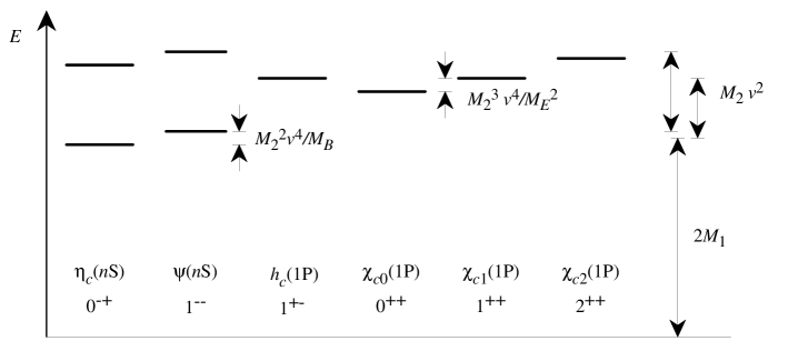
The interesting gross feature of the spectrum is not the overall mass gapโ€”close to $2M_{1}$โ€”but the pattern of radial and orbital excitations, e.g.ย m2โ€‹Sโˆ’m1โ€‹Ssubscript๐‘š2Ssubscript๐‘š1Sm_{\rm 2S}-m_{\rm 1S} or $m_{\rm 1P}-m_{\rm 1S}$. These splittings are dictated by the kinetic massย M2subscript๐‘€2M_{2}. Following the analysis of ref.ย [12] they are of orderย M2โ€‹v2subscript๐‘€2superscript๐‘ฃ2M_{2}v^{2}, whereย v๐‘ฃv is the typical velocity of a heavy quark in quarkonium. ($v\sim 0.3$ for charmonium, and $v\sim 0.1$ for bottomonium.) Further application of the velocity counting in ref.ย [12] to eq.ย (9.1) shows that the hyperfine splittings are $\mbox{\boldmath$\Sigma$}\!\cdot\!\mbox{\boldmath$B$}/M_{B}\sim M_{2}^{2}v^{4}/M_{B}$, and the spin-orbit splittings are $[\mbox{\boldmath$\gamma$}\!\cdot\!\mbox{\boldmath$D$},\mbox{\boldmath$\gamma$}\!\cdot\!\mbox{\boldmath$E$}]/M_{E}^{2}\sim M_{2}^{3}v^{4}/M_{E}^{2}$.

The preceding paragraph merely reviews the well-known argument that the rest mass of a nonrelativistic particle decouples from the interesting dynamics. In our formalism the reasoning suggests the following strategy: forget about $M_{1}$ and adjust the bare mass so that the kinetic massย M2subscript๐‘€2M_{2} takes the physical value. Meanwhile, choose the couplingย ฮถ๐œ\zeta by convenience. The obvious example is to take $\zeta=1$, as in the Wilson and Sheikholeslami-Wohlert actions.

Since the Wilson and Sheikholeslami-Wohlert actions represent viable nonrelativistic field theories, it makes sense to compare them to the explicitly nonrelativistic theories. The (tree-level) masses for the Wilson action are plotted as a function ofย m0โ€‹asubscript๐‘š0๐‘Žm_{0}a in fig.ย 3.

Refer to caption
Figure 3: The (tree-level) masses for Wilson fermions ($\zeta=1$, rs=1subscript๐‘Ÿ๐‘ 1r_{s}=1). By happenstance $M_{2}$ is always within 15% of $m_{0}$, which is a result of a conspiracy between the $\mbox{\boldmath$\gamma$}\!\cdot\!\mbox{\boldmath$D$}$ and Wilson terms.

Assuming $m_{0}a$ is chosen so that $M_{2}=m_{q}$, the other masses satisfy $M_{1}<m_{q}$, $M_{B}^{-1}<m_{q}^{-1}$, and $M_{E}^{-1}<m_{q}^{-1}$. The simplest form of nonrelativistic QCDย [11] has Hamiltonian $\hat{H}_{\rm NR}=\hat{\bar{\Psi}}\mbox{\boldmath$D$}^{2}\hat{\Psi}/(2m_{q})$. Thus, in our notation, $\hat{H}_{\rm NR}$ has $M_{1}=0$ and $M_{B}^{-1}=M_{E}^{-1}=0$. Thus, the Hamiltonians of the Wilson and simplest nonrelativistic theories make the same errors qualitatively. For example, in both one expects the fine and hyperfine splittings to be too small. Similarly, for the Sheikholeslami-Wohlert action one finds $M_{B}=M_{2}$, and thus good hyperfine splittings, but $M_{E}^{-1}>m_{q}^{-1}$, so the splittings between $\chi_{J}$ states ought to be too large. To obtain the correct spin-orbit splittings, one needs the mass dependence ofย cEsubscript๐‘๐ธc_{E}, cf.ย Appendixย A.

A parallel set of remarks applies to heavy-light systems. The Hamiltonian of the lattice theory satisfies the usual heavy-quark symmetries as mqโ†’โˆžโ†’subscript๐‘š๐‘žm_{q}\to\infty, no matter what M2subscript๐‘€2M_{2},ย MBsubscript๐‘€๐ตM_{B}, andย MEsubscript๐‘€๐ธM_{E} are. On the other hand, the lattice theory possesses the right151515Many phenomenological applications require matrix elements of operators of the electroweak Hamiltonian. These operators must also be constructed to the appropriate order in 1/mQ1subscript๐‘š๐‘„1/m_{Q}, cf.ย sect.ย 7. In particular, to first order in 1/mQ1subscript๐‘š๐‘„1/m_{Q} the coefficient d1subscript๐‘‘1d_{1} must be chosen according to eq.ย (7.10). 1/mQ1subscript๐‘š๐‘„1/m_{Q} corrections only if M2=MB=mQsubscript๐‘€2subscript๐‘€๐ตsubscript๐‘š๐‘„M_{2}=M_{B}=m_{Q}. Aย computation with the Wilson action and mQ=M2subscript๐‘š๐‘„subscript๐‘€2m_{Q}=M_{2} obtains spin-averaged features correctly, but underestimates the chromomagnetic 1/mQ1subscript๐‘š๐‘„1/m_{Q} corrections. Compared to corrections from the kinetic energy, the spin dependent effects are thought to be smallย [17], so again the most essential adjustment is M2=mQsubscript๐‘€2subscript๐‘š๐‘„M_{2}=m_{Q}. Aย better computation with the Sheikholeslami-Wohlert action and mQ=M2=MBsubscript๐‘š๐‘„subscript๐‘€2subscript๐‘€๐ตm_{Q}=M_{2}=M_{B} obtains all1515footnotemark: 15 1/mQ1subscript๐‘š๐‘„1/m_{Q} features correctly.

Despite the similarity between previous nonrelativistic field theoriesย [8, 9, 10, 11, 12] and the view adopted in this section, there are significant technical differences. The four-component approach explicitly includes the termsย m0โ€‹ฯˆยฏโ€‹(x)โ€‹ฯˆโ€‹(x)subscript๐‘š0ยฏ๐œ“๐‘ฅ๐œ“๐‘ฅm_{0}\bar{\psi}(x)\psi(x) and terms that couple upper and lower components, such asย ฯˆยฏโ€‹(x)โ€‹๐œธโ‹…๐‘ซโ€‹ฯˆโ€‹(x)โ‹…ยฏ๐œ“๐‘ฅ๐œธ๐‘ซ๐œ“๐‘ฅ{\bar{\psi}(x)\mbox{\boldmath$\gamma$}\!\cdot\!\mbox{\boldmath$D$}\psi(x)} andย ฯˆยฏโ€‹(x)โ€‹๐œถโ‹…๐‘ฌโ€‹ฯˆโ€‹(x)โ‹…ยฏ๐œ“๐‘ฅ๐œถ๐‘ฌ๐œ“๐‘ฅ{\bar{\psi}(x)\mbox{\boldmath$\alpha$}\!\cdot\!\mbox{\boldmath$E$}\psi(x)}. The program of Lepage, et al,ย [12] omits these interactions in practice, though perhaps not in principle. There are advantages to leaving out the Dirac blockโ€“off-diagonal interactions. Fermion propagators are the solution of a (one-sweep) initial-value problem, whereas they are otherwise the solution of a boundary-value problem, solvable only by iteration; with fewer interactions, perturbation theory is easierย [27]. On the other hand, these interactions are necessary to takeย aโ†’0โ†’๐‘Ž0a\to 0 (by brute force) without the scourge of power-law divergences, or to reach into the semirelativistic regime.

10 Numerical Tests and Applications

With a few examples this section tests the results of the previous sections with Monte Carlo data. All data were generated with the axis-interchange symmetric Wilson or Sheikholeslami-Wohlert actions, so as mqโ€‹asubscript๐‘š๐‘ž๐‘Žm_{q}a increases, we rely on the nonrelativistic interpretation of sect.ย 9. The tests verify the most important lessons. The bare mass should be adjusted until the kinetic massย M2subscript๐‘€2M_{2}, defined in eq.ย (4.7), takes the desired value. In particular, in an extrapolation to vanishing lattice spacing, one ought to hold the kinetic mass161616This can be done nonperturbatively with a meson instead of a quark state. fixed. On the other hand, the dynamically irrelevant rest mass may deviate fromย mqsubscript๐‘š๐‘žm_{q}. For matrix elements, it is also important to use the improved fieldย ฮจIsubscriptฮจI\Psi_{\rm I} of eq.ย (7.8) orย (A.17). The factor eM1โ€‹a/2superscript๐‘’subscript๐‘€1๐‘Ž2e^{M_{1}a/2} is more important than the bracket in eq.ย (7.8), because it guarantees a smooth approach to the static limit.171717Neglecting the bracket introduces only Oโ€‹(m0โ€‹pโ€‹pโ€‹a2)Osubscript๐‘š0๐‘๐‘superscript๐‘Ž2{\rm O}(m_{0}\hbox to0.0pt{$\hskip 0.50003ptp$\hss}p\hskip 0.50003pta^{2}) lattice artifacts at m0โ€‹aโ‰ช1much-less-thansubscript๐‘š0๐‘Ž1m_{0}a\ll 1, but Oโ€‹(pโ€‹p/mq)O๐‘๐‘subscript๐‘š๐‘ž{\rm O}(\hbox to0.0pt{$\hskip 0.50003ptp$\hss}p\hskip 0.50003pt/m_{q}) atย m0โ€‹aโ€‹โˆผ>1subscript๐‘š0๐‘Žโˆผ>1m_{0}a\mathop{\raisebox{-1.72218pt}{\hbox to0.0pt{$\sim$\hss}}\raisebox{1.72218pt}{$>$}}1.

First, consider the mass spectrum, in particular the hyperfine splitting in heavy-light systems. By heavy-quark spin symmetry the vector-pseudoscalar mass differenceย mVโˆ’mPsubscript๐‘š๐‘‰subscript๐‘š๐‘ƒ{m_{V}-m_{P}} is expected to be proportional toย 1/mQ1subscript๐‘š๐‘„1/m_{Q}. Obviously the leading term in the sum ${m_{V}+m_{P}}$ is proportional toย mQsubscript๐‘š๐‘„m_{Q}, so the combination ${m_{V}^{2}-m_{P}^{2}}$ should be nearly independent ofย mQsubscript๐‘š๐‘„m_{Q}. Numerical workย [28, 29] found, however, that ${m_{V}^{2}-m_{P}^{2}}$ decreases for increasingย mQsubscript๐‘š๐‘„m_{Q}, with lattice spacingย a๐‘Ža held fixed. These analyses take $m_{V}$ andย mPsubscript๐‘š๐‘ƒm_{P} from the rest mass. From sect.ย 9 the rest massย M1subscript๐‘€1M_{1} of the quark governs the rest mass of the mesons, while the chromomagnetic massย MBsubscript๐‘€๐ตM_{B} governs the hyperfine splitting. The computed lattice quantity, therefore, is proportional toย M1/MBsubscript๐‘€1subscript๐‘€๐ตM_{1}/M_{B}, which decreases for increasing quark mass, cf.ย fig.ย 3. Given $M_{1}$, $M_{B}$ is not as large with the Sheikholeslami-Wohlert action as with the Wilson action. Numerical data withย cB=1subscript๐‘๐ต1c_{B}=1 show behaviorย [29] qualitatively similar toย cB=0subscript๐‘๐ต0c_{B}=0.

To improve the determination ofย mVโˆ’mPsubscript๐‘š๐‘‰subscript๐‘š๐‘ƒ{m_{V}-m_{P}} one should tune to the kinetic mass instead of the rest mass and use the mean-field or one-loop estimate ofย cBsubscript๐‘๐ตc_{B}. The chosen value ofย cBsubscript๐‘๐ตc_{B} could be tested in quarkonia. Then in heavy-light systems one could verify two predictions of heavy-quark symmetry, as applied to the lattice theory: a falling $M_{1}/M_{B}$ behavior when using the mesonsโ€™ rest masses, and a flat $M_{2}/M_{B}$ behavior when using the mesonsโ€™ kinetic masses.

Next, consider the improvement and normalization of multi-quark operators from sect.ย 7. The normalization of the vector current can be checked nonperturbatively. The fermion number

Nhโ€‹(H)=โŸจH|2โ€‹ฮบtโ€‹ZVโ€‹ฯˆยฏxhโ€‹ฮณ0โ€‹ฯˆxh|HโŸฉ=โŸจฮฆHโ€‹2โ€‹ฮบtโ€‹ZVโ€‹ฯˆยฏxhโ€‹ฮณ0โ€‹ฯˆxhโ€‹ฮฆHโ€ โŸฉโŸจฮฆHโ€‹ฮฆHโ€ โŸฉsubscript๐‘โ„Ž๐ปquantum-operator-product๐ป2subscript๐œ…๐‘กsubscript๐‘๐‘‰superscriptsubscriptยฏ๐œ“๐‘ฅโ„Žsubscript๐›พ0superscriptsubscript๐œ“๐‘ฅโ„Ž๐ปdelimited-โŸจโŸฉsubscriptฮฆ๐ป2subscript๐œ…๐‘กsubscript๐‘๐‘‰superscriptsubscriptยฏ๐œ“๐‘ฅโ„Žsubscript๐›พ0superscriptsubscript๐œ“๐‘ฅโ„Žsuperscriptsubscriptฮฆ๐ปโ€ delimited-โŸจโŸฉsubscriptฮฆ๐ปsuperscriptsubscriptฮฆ๐ปโ€ N_{h}(H)=\langle H|2\kappa_{t}Z_{V}\bar{\psi}_{x}^{h}\gamma_{0}\psi_{x}^{h}|H\rangle=\frac{\langle\Phi_{H}2\kappa_{t}Z_{V}\bar{\psi}_{x}^{h}\gamma_{0}\psi_{x}^{h}\Phi_{H}^{\dagger}\rangle}{\langle\Phi_{H}\Phi_{H}^{\dagger}\rangle} (10.1)

counts the number of $h$-flavored fermions in $|H\rangle$. If $|H\rangle$ has one and only oneย hโ„Žh in it, the conditionย Nh=1subscript๐‘โ„Ž1N_{h}=1 defines the factorย 2โ€‹ฮบtโ€‹ZV2subscript๐œ…๐‘กsubscript๐‘๐‘‰2\kappa_{t}Z_{V}.181818In the notation of sect.ย 8, $Z_{V}=Z_{\gamma_{\mu}}$ and $Z_{A}=Z_{\gamma_{\mu}\gamma_{5}}$. Fig.ย 4 compares this nonperturbative definition
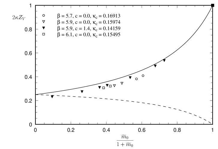
Refer to caption
Figure 4: The charge normalization factor $2\kappa Z_{V}$ vs.ย (ฮบcโˆ’ฮบ)/(ฮบcโˆ’3โ€‹ฮบ/4)=(1โˆ’8โ€‹ฮบ~)/(1โˆ’6โ€‹ฮบ~)=m~0/(1+m~0)subscript๐œ…๐‘๐œ…subscript๐œ…๐‘3๐œ…418~๐œ…16~๐œ…subscript~๐‘š01subscript~๐‘š0(\kappa_{c}-\kappa)/(\kappa_{c}-3\kappa/4)=\linebreak(1-8\tilde{\kappa})/(1-6\tilde{\kappa})=\widetilde{m}_{0}/(1+\widetilde{m}_{0}), with $u_{0}=1/8\kappa_{c}$. The symbols are Monte Carlo determinations with rs=ฮถ=1subscript๐‘Ÿ๐‘ ๐œ1r_{s}=\zeta=1 andย cB=cE=csubscript๐‘๐ตsubscript๐‘๐ธ๐‘c_{B}=c_{E}=c. The solid square is the exact result for $\kappa=0$. The solid curve is the mean-field approximation to eq.ย (7.7), $2\kappa Z_{V}=1-6\tilde{\kappa}$. The dashed curve is a mean-field Ansatz $2\tilde{\kappa}$, which (foolishly) neglects the mass dependence.

ofย 2โ€‹ฮบโ€‹ZV2๐œ…subscript๐‘๐‘‰2\kappa Z_{V} with the mean-field-improved, tree-level perturbative approximation. The symbols are from Monte Carlo calculationsย [30] of eq.ย (10.1), with $|H\rangle$ a meson with a spectator anti-quark of different flavor, and the solid curve is the mean-field improved, tree-level approximationย 2โ€‹ฮบโ€‹(1+m~0โ€‹h)2๐œ…1subscript~๐‘š0โ„Ž2\kappa(1+\widetilde{m}_{0h}). Fig.ย 4 exhibits several interesting features. The solid curve accurately tracks the dominant mass dependence fromย m~0=0subscript~๐‘š00\widetilde{m}_{0}=0 toย m~0=โˆžsubscript~๐‘š0\widetilde{m}_{0}=\infty. From eq.ย (8.10) one expects a subdominant mass dependence from loop correctionsย ZV[l]โ€‹(m0โ€‹hโ€‹a)subscriptsuperscript๐‘delimited-[]๐‘™๐‘‰subscript๐‘š0โ„Ž๐‘ŽZ^{[l]}_{V}(m_{0h}a). Indeed, near $\widetilde{m}_{0}=0$ the massless one-loop correctionย [31, 32] accounts quantitatively for the discrepancy, and near $\widetilde{m}_{0}=\infty$ the discrepancy becomes smaller, in accord with a Ward identity, which requiresย 2โ€‹ฮบโ€‹ZV=12๐œ…subscript๐‘๐‘‰12\kappa Z_{V}=1 at infinite massย [33]. Neglecting the dominant mass dependence, as in the dashed curve, is obviously completely wrong for $\widetilde{m}_{0}\mathop{\raisebox{-1.72218pt}{\hbox to0.0pt{$\sim$\hss}}\raisebox{1.72218pt}{$>$}}1$.

Finally, consider the decay constant of a heavy-light pseudoscalar meson, computed with the local axial current $J^{ub}_{\mu 5}(x)=\bar{\psi}^{u}(x)\gamma_{\mu}\gamma_{5}\psi^{b}(x)$. Fig.ย 5 shows Monte Carlo dataย [34, 35]

Refer to caption
Figure 5: $\phi_{P}=\sqrt{m_{P}}f_{P}$ vs.ย 1/mq1subscript๐‘š๐‘ž1/m_{q}. Squares represent results from the conventional zero-mass normalization, plotted versusย 1/M11subscript๐‘€11/M_{1}. Circles represent the same results with the correct normalization, plotted versusย 1/M21subscript๐‘€21/M_{2}. The points for $m_{q}^{-1}>0$ are obtained with the Wilson actionย [34]. The static ($m_{q}^{-1}=0$) point is from Ref.ย [35]. The curves guide the eye, and the approximate location of the physical $B$ and $D$ mesons is shown.

atย ฮฒ=5.7๐›ฝ5.7\beta=5.7 (for which $a^{-1}\approx 1$ย GeV) for

$$\phi_{P}=\sqrt{2}\,\langle 0|Z_{A}^{ub}J^{ub}_{\mu 5}|P,{\bf 0}\rangle=\sqrt{m_{P}}f_{P}v_{\mu},$$ (10.2)

where $v_{\mu}$ is the mesonโ€™s four-velocity. (The vacuum and one-meson states are normalized to unity.) We have deliberately chosen a largish lattice spacing to enhance lattice artifacts, and thus test our control over them. We analyze the data two different ways. The lower set of points takes the meson mass from the rest mass and neglects the factor1818footnotemark: 18 $Z_{A}^{ub}=e^{M_{1b}a/2}$ in eq.ย (7.8). As suggested by the curve, the neglectful analysis would produce a locus of points that approaches zero in the static limit. The upper set of points uses the normalization factor, andโ€”just as importantโ€”it defines the meson mass through a mean-field approximation to the kinetic mass.191919Ref.ย [34] provides hopping parameters and rest masses only, but the mean-field approximation is adequate for illustrative purposes. Fig.ย 5 shows how crucial both refinements are, if the Wilson-action data are to approach the static limit smoothly.

An important application of a plot like fig.ย 5 is to compute the slope in $1/m_{q}$. In the heavy-quark effective theory the slope is seen to arise from three sources: the kinetic energy, the chromomagnetic interaction, and a correction to the infinite-mass currentย [17]. The lattice theory has direct analogs: the kinetic energy requires tuningย M2=mqsubscript๐‘€2subscript๐‘š๐‘žM_{2}=m_{q}, the chromomagnetic contribution requires tuningย MB=mqsubscript๐‘€๐ตsubscript๐‘š๐‘žM_{B}=m_{q}, and the local lattice current requires a correction, given most compactly by eqs.ย (7.8) andย (7.10). All three ingredients are needed to obtain the correct slopeย [36].

11 Conclusions

This paper (and conference reportsย [37, 18, 36] anticipating it) provides the foundations of a theory of lattice fermions, valid at any massโ€”large or small. The action starts with a set of interactions that encompasses those of both light-fermion actionsย [13, 6] and heavy-fermion actionsย [10, 11, 12]. The couplings of such a general action are then tuned in successive approximations to the renormalized trajectory. In applying renormalization-group techniques to analyze and reduce cutoff effects we do not, however, expand in eitherย mqโ€‹asubscript๐‘š๐‘ž๐‘Žm_{q}a orย ฮ›QCD/mqsubscriptฮ›QCDsubscript๐‘š๐‘ž\Lambda_{\rm QCD}/m_{q}.

Although there are several methods for tuning the action (for example, refs.ย [38, 39]), our analysis is based on Symanzik-like, on-shell improvement criteria. This entails the computation of on-shell correlation functions, or, equivalently, of the Hamiltonian. Enforcing continuum-limit behaviorโ€”for example the relativistic mass shellโ€”yields conditions on couplings of higher-dimension interactions. In practice, we here compute on-shell quantities in (tadpole-improved) perturbation theory.

An examination of the lattice theoryโ€™s Hamiltonian, derived from the transfer matrix, is especially illuminating. It shows that it is unnecessary to improve Wilsonโ€™s discretization of the time derivative. Instead higher-dimension interactions can be built from fields on one (or, in some cases, two adjacent) timeslices. Thus, our class of improved lattice actions automatically has an easy-to-construct transfer matrix. The actions, consequently, all automatically satisfy heavy-quark symmetries in the limit of large mass.

The Hamiltonian is a useful tool for examining lattice artifacts. A term of dimension s+4๐‘ 4s+4 factorizes as

ฮดโ€‹H^lat=asโ€‹bโ€‹(mqโ€‹a,g2)โ€‹H^,๐›ฟsubscript^๐ปlatsuperscript๐‘Ž๐‘ ๐‘subscript๐‘š๐‘ž๐‘Žsuperscript๐‘”2^๐ป\delta\hat{H}_{\rm lat}=a^{s}b(m_{q}a,g^{2})\hat{H}, (11.1)

with dependence on the theoryโ€™s relevant couplings, mqโ€‹asubscript๐‘š๐‘ž๐‘Žm_{q}a andย g2superscript๐‘”2g^{2}, in the coefficientย b๐‘b. From this expression it is plain how the artifacts behave as the mass increases: the absolute error induced by eq.ย (11.1) isย โŸจฮดโ€‹H^latโŸฉโˆผ(๐’‘โ€‹a)sโ€‹๐’‘similar-todelimited-โŸจโŸฉ๐›ฟsubscript^๐ปlatsuperscript๐’‘๐‘Ž๐‘ ๐’‘\langle\delta\hat{H}_{\rm lat}\rangle\sim(\mbox{\boldmath$p$}a)^{s}\mbox{\boldmath$p$}, whereย ๐’‘๐’‘p is the typical three-momentum of the process. At small mass it is standard that the associated coefficient is a benign numerical factorย bโ€‹(0)๐‘0b(0). At large mass the lattice actionโ€™s heavy-quark symmetry implies that it is a (generally different) numerical factorย bโ€‹(โˆž)๐‘b(\infty). Our explicit results at tree level and our analysis of higher orders show thatย bโ€‹(mqโ€‹a)๐‘subscript๐‘š๐‘ž๐‘Žb(m_{q}a) is a smooth, gentle function connecting the two extremes. In a nutshell, therefore, the characteristic measures of cutoff artifacts areย ฮ›QCDโ€‹asubscriptฮ›QCD๐‘Ž\Lambda_{\rm QCD}a andย ๐’‘โ€‹a๐’‘๐‘Ž\mbox{\boldmath$p$}a, but never mqโ€‹asubscript๐‘š๐‘ž๐‘Žm_{q}a.

In general our actions have two hopping parameters. Then it is possible to maintain equality between the rest mass (energy at zero momentum, eq.ย (4.6)) and the kinetic mass (inertial response, eq.ย (4.7)). In nonrelativistic systems, however, there is a noteworthy simplification. Embracing the philosophy of the staticย [8] or nonrelativisticย [10, 11] theories, one can ignore the rest mass and, hence, forgo one of the hopping parameters. The obvious application is to set them equal, as in the Wilsonย [3] and Sheikholeslami-Wohlertย [6] actions. Therefore, the correct interpretation of numerical data generated with these actions atย mqโ€‹aโˆผ1similar-tosubscript๐‘š๐‘ž๐‘Ž1m_{q}a\sim 1 is a nonrelativistic one. In particular, the hopping parameter must be adjusted so that the kinetic mass agrees with the physical mass.

If one knows a priori that a quark is nonrelativistic, it is computationally cheaper to use a two-component formalismย [12]. But there are many instances in which one would like to trace the mass dependence from the static limit down to, say, the strange quark. One example is fig.ย 5, which, with reliable calculations, should indicate how and where the heavy-quark expansion deteriorates.

The results of this paper can be extended in several ways. The couplings have been computed at tree level with mean-field improvement. One-loop calculations are desirable, and better still would be a nonperturbative determination, perhaps in a mass-dependent generalization of ref.ย [40]. Once one is confident that ${\rm O}(a)$ artifacts are under control, one can extend the analysis to dimension-six interactions. Tree-level, ${\rm O}(a^{2})$ improvement should be manageable; beyond tree level the bothersome four-fermion interactions enter the fray.

One would like to use the actions presented here in Monte Carlo calculations of QCD. If one uses the ${\rm O}(v^{4})$-improved action to compute the spectrum of charmonium and bottomonium, then, without more tuning, one could calculate properties of $D$ย and $B$ย mesons, including the electroweak matrix elements needed to determine the unknown elements of the Cabibbo-Kobayashi-Maskawa matrix.202020For relevant reviews, see ref.ย [41, 21]. Note that for these matrix elements, as well as for the quark mass in the ${\overline{\rm MS}}$ scheme, a small lattice spacing is helpful to reduce perturbative corrections. Once the lattice spacing is small enough so that $m_{Q}a\mathop{\raisebox{-1.72218pt}{\hbox to0.0pt{$\sim$\hss}}\raisebox{1.72218pt}{$<$}}1$, our formulation is especially advantageous. The two-component nonrelativistic theory breaks down asย mQโ€‹asubscript๐‘š๐‘„๐‘Žm_{Q}a gets smallerย [11], yet the old small-mass theory would have leading lattice artifacts of orderย ฮฑsโ€‹mQโ€‹asubscript๐›ผ๐‘ subscript๐‘š๐‘„๐‘Ž\alpha_{s}m_{Q}a and $(m_{Q}a)^{2}$. Our improved action, on the other hand, remains viable for any mass, and its cutoff effects are small, of orderย ฮฑsโ€‹ฮ›QCDโ€‹asubscript๐›ผ๐‘ subscriptฮ›QCD๐‘Ž\alpha_{s}\Lambda_{\rm QCD}a andย (ฮ›QCDโ€‹a)2superscriptsubscriptฮ›QCD๐‘Ž2(\Lambda_{\rm QCD}a)^{2}. To obtain comparable accuracy through brute force in the old theory, one would have to reduce the lattice spacing by a factor of $m_{Q}/\Lambda_{\rm QCD}$โ€”about five for the charm quark. Even for a perfect algorithm the savings in computer time is, therefore, a factor of $5^{4}$.

Acknowledgements

We would like to thank Peter Lepage for numerous discussions and Bart Mertens for collaboration on the one-loop calculations mentioned in sect.ย 8. During this work we have also had useful conversations with Claude Bernard, Estia Eichten, Jim Labrenz, Martin Lรผscher, Maarten Golterman, and Jim Simone. AXK would like to thank the Fermilab Theory Group for hospitality. Fermilab is operated by Universities Research Association, Inc., under contract DE-AC02-76CH03000 with the U.S. Department of Energy.

Appendix A Quarkonium to ${\rm O}(v^{4})$

This appendix extends the analysis of the main text to incorporate interactions that contribute in quarkonium throughย Oโ€‹(v4)Osuperscript๐‘ฃ4{\rm O}(v^{4}). Naively, this would entail close scrutiny of all interactions through ${\rm O}(\mbox{\boldmath$p$}^{4})$, i.e.ย up to dimension seven. Some dimension-seven bilinear interactions are listed in Tableย 5,

Table 5: Estimates of the size of the dimension-seven interactions that arise in designing an action for quarkonia with an accuracy of $m_{Q}v^{4}$. (There are many other interactions needed to ensure ${\rm O}((\Lambda_{\rm QCD}a)^{4})$ accuracy in all-light and heavy-light systems.)
$H_{n}$ only light heavy-light quarkonia
$\bar{\Psi}(\mbox{\boldmath$D$}^{2})^{2}\Psi$ $\Lambda_{\rm QCD}^{4}$ $\Lambda_{\rm QCD}^{4}$ $m_{Q}^{4}v^{4}$
$\bar{\Psi}D_{i}^{4}\Psi$ $\Lambda_{\rm QCD}^{4}$ $\Lambda_{\rm QCD}^{4}$ $m_{Q}^{4}v^{4}$

with their magnitude in quarkonium estimated by the velocity-counting rules of ref.ย [12]. Together with Tableย 3, one sees that not all dimension-six and -seven interactions are necessary toย Oโ€‹(v4)Osuperscript๐‘ฃ4{\rm O}(v^{4}); this Appendix considers only the entries that are.

One must consider the dimension-six interaction

Sso=csoโ€‹ฮบsโ€‹โˆ‘nฯˆยฏnโ€‹ฮณ0โ€‹[๐œธโ‹…๐‘ซ,๐œธโ‹…๐‘ฌ]โ€‹ฯˆn,subscript๐‘†sosubscript๐‘sosubscript๐œ…๐‘ subscript๐‘›subscriptยฏ๐œ“๐‘›subscript๐›พ0โ‹…๐œธ๐‘ซโ‹…๐œธ๐‘ฌsubscript๐œ“๐‘›S_{\rm so}=c_{\rm so}\kappa_{s}\sum_{n}\bar{\psi}_{n}\gamma_{0}[\mbox{\boldmath$\gamma$}\!\cdot\!\mbox{\boldmath$D$},\mbox{\boldmath$\gamma$}\!\cdot\!\mbox{\boldmath$E$}]\psi_{n}, (A.1)

with coupling $c_{\rm so}$, and the dimension-six and -seven interactions

S4=โˆ’2โ€‹ฮบsโ€‹โˆ‘nฯˆยฏnโ€‹[c4โ€‹Dโ€‹๐œธโ‹…๐‘ซโˆ’12โ€‹rsโ€‹c4โ€‹Lโ€‹โ–ณ(3)]โ€‹โ–ณ(3)โ€‹ฯˆn,subscript๐‘†42subscript๐œ…๐‘ subscript๐‘›subscriptยฏ๐œ“๐‘›delimited-[]โ‹…subscript๐‘4๐ท๐œธ๐‘ซ12subscript๐‘Ÿ๐‘ subscript๐‘4๐ฟsuperscriptโ–ณ3superscriptโ–ณ3subscript๐œ“๐‘›S_{4}=-2\kappa_{s}\sum_{n}\bar{\psi}_{n}\left[c_{4D}\mbox{\boldmath$\gamma$}\!\cdot\!\mbox{\boldmath$D$}-\,\mbox{\small$\frac{1}{2}$}r_{s}c_{4L}\triangle^{(3)}\right]\triangle^{(3)}\psi_{n}, (A.2)

with couplings $c_{4D}$ and $c_{4L}$. Further dimension-six and -seven interactions contribute in ${\rm O}(v^{6})$ or higherย [12]. We discuss the adjustment of $c_{\rm so}$ in eq.ย (A.1) in sect.ย A.1, and the adjustment of $c_{4D}$ and $c_{4L}$ in eq.ย (A.2) in sect.ย A.2.

The discretization of the covariant differenceย ๐‘ซ๐‘ซD and Laplacianย โ–ณ(3)superscriptโ–ณ3\triangle^{(3)} also must be improved, to remove $\bar{\Psi}\gamma_{i}D_{i}^{3}\Psi$ and $\bar{\Psi}D_{i}^{4}\Psi$, respectively. These interactions break rotational invariance, and we treat them in sect.ย A.2.

A.1 Chromoelectric interactions to ${\rm O}(v^{4})$

It is easiest to treat the โ€œspin-orbitโ€ interactionย Ssosubscript๐‘†soS_{\rm so} in the Hamiltonian formalism of sect.ย 5. The coupling $c_{\rm so}$ can only appear in a dimension-six term implied by the ellipsis in eq.ย (5.16). The spin-orbit Hamiltonian is

$$\hat{H}_{\rm so}=a^{2}b_{\rm so}(m_{0}a)\hat{\bar{\Psi}}\gamma_{0}[\mbox{\boldmath$\gamma$}\!\cdot\!\mbox{\boldmath$D$},\mbox{\boldmath$\gamma$}\!\cdot\!\mbox{\boldmath$E$}]\hat{\Psi}.$$ (A.3)

Under the two-parameter Foldy-Wouthuysen-Tani transformation of eq.ย (5.23)

$$b^{\prime}_{\rm so}=b_{\rm so}-\mbox{\small$\frac{1}{2}$}\xi_{1}^{2}+b_{E}\xi_{1}+b_{1}\xi_{E}-2m_{q}ab_{0}\xi_{1}\xi_{E}.$$ (A.4)

With $b_{\rm so}$ it is possible to give an invariant involving $b_{E}$:

$$B_{E}=b_{1}^{2}-4m_{q}ab_{0}b_{1}b_{E}-8(m_{q}ab_{0})^{2}b_{\rm so}={b^{\prime}_{1}}^{2}-4m_{q}ab^{\prime}_{0}b^{\prime}_{1}b^{\prime}_{E}-8(m_{q}ab^{\prime}_{0})^{2}b^{\prime}_{\rm so},$$ (A.5)

and one wants $B_{E}=1$. Just as the redundancy associated with the Foldy-Wouthuysen-Tani parameterย ฮพ1subscript๐œ‰1\xi_{1} intertwines the mass dependence ofย ฮถ๐œ\zeta andย rssubscript๐‘Ÿ๐‘ r_{s}, the redundancy associated with the other Foldy-Wouthuysen-Tani parameterย ฮพEsubscript๐œ‰๐ธ\xi_{E} intertwines the mass dependence ofย cEsubscript๐‘๐ธc_{E} andย csosubscript๐‘soc_{\rm so} too.

Assuming a discretization of $S_{\rm so}$ that resides on two timeslices only, it is straightforward to generalize the transfer-matrix construction to the action $S_{0}+S_{B}+S_{E}+S_{\rm so}$. After expanding the transfer matrix in powers ofย a๐‘Ža one finds

$$\begin{array}[]{r@{\;=\;}l}b_{\rm so}&-\mbox{\small$\frac{1}{2}$}(1-c_{E})\zeta^{2}f_{2}(m_{0})+{\displaystyle\frac{c_{\rm so}\zeta}{2(1+m_{0})}}.\end{array}$$ (A.6)

Combining eqs.ย (A.5), (5.29), andย (A.6) and setting $B_{E}=1$ yields the mass-dependent condition

cE=ฮถ2โˆ’1m0โ€‹(2+m0)+rsโ€‹ฮถ1+m0+rs2โ€‹m0โ€‹(2+m0)4โ€‹(1+m0)2+csoโ€‹m0โ€‹(2+m0)ฮถโ€‹(1+m0).subscript๐‘๐ธsuperscript๐œ21subscript๐‘š02subscript๐‘š0subscript๐‘Ÿ๐‘ ๐œ1subscript๐‘š0superscriptsubscript๐‘Ÿ๐‘ 2subscript๐‘š02subscript๐‘š04superscript1subscript๐‘š02subscript๐‘sosubscript๐‘š02subscript๐‘š0๐œ1subscript๐‘š0c_{E}=\frac{\zeta^{2}-1}{m_{0}(2+m_{0})}+\frac{r_{s}\zeta}{1+m_{0}}+\frac{r_{s}^{2}m_{0}(2+m_{0})}{4(1+m_{0})^{2}}+\frac{c_{\rm so}m_{0}(2+m_{0})}{\zeta(1+m_{0})}. (A.7)

Here the rest massย M1subscript๐‘€1M_{1} has been eliminated in favor of the kinetic massย M2subscript๐‘€2M_{2} as appropriate to the nonrelativistic interpretation of sect.ย 9.

The redundant direction associated to $\xi_{E}$ permits a free choice ofย csosubscript๐‘soc_{\rm so}. In our framework, which stresses a smooth matching to the massless limit, the most convenient choice is probably $c_{\rm so}=0$. But for purely nonrelativistic applications ref.ย [12] would choose $c_{E}=0$ and $\zeta c_{\rm so}\propto m_{q}^{-2}$. Other possibilities correspond to the special choice forย rssubscript๐‘Ÿ๐‘ r_{s} in eq.ย (5.35). Then eq.ย (A.7) reduces to

$$c_{E}=1+2\log(1+m_{0})c_{\rm so}.$$ (A.8)

The further special case corresponding to $\xi_{E}=0$ is $c_{E}=1$ (independent ofย m0โ€‹asubscript๐‘š0๐‘Žm_{0}a) and $c_{\rm so}=0$.

A.2 Kinetic energy to ${\rm O}(v^{4})$

The interactionย S4subscript๐‘†4S_{4} produces corrections to the kinetic energy. It is easiest to analyze from the energy-momentum relation, as in sect.ย 4. Expanding eq.ย (4.4) to ${\rm O}(\mbox{\boldmath$p$}^{4})$ yields

$$E=M_{1}+\frac{\mbox{\boldmath$p$}^{2}}{2M_{2}}-{\textstyle\frac{1}{6}}w_{4}a^{2}\sum_{i}p_{i}^{4}-\frac{(\mbox{\boldmath$p$}^{2})^{2}}{8M_{4}^{3}}+\ldots,$$ (A.9)

where

M4=โˆ’(โˆ‚4Eโˆ‚pi2โ€‹โˆ‚pj2)pโ€‹p=๐ŸŽโˆ’1/3,iโ‰ jformulae-sequencesubscript๐‘€4subscriptsuperscriptsuperscript4๐ธsuperscriptsubscript๐‘๐‘–2superscriptsubscript๐‘๐‘—213๐‘๐‘0๐‘–๐‘—M_{4}=-\left(\frac{\partial^{4}E}{\partial p_{i}^{2}\partial p_{j}^{2}}\right)^{-1/3}_{\hbox to0.0pt{$\hskip 0.35002pt\scriptstyle p$\hss}\scriptstyle p\hskip 0.35002pt={\bf 0}},\quad i\neq j (A.10)

and

$$w_{4}=-\frac{1}{4}\left.\frac{\partial^{4}E}{\partial p_{i}^{4}}\right|_{\hbox to0.0pt{$\hskip 0.35002pt\scriptstyle p$\hss}\scriptstyle p\hskip 0.35002pt={\bf 0}}-\frac{3}{4M_{4}^{3}}.$$ (A.11)

The relativistic mass shell satisfies $M_{4}=M_{2}=M_{1}$, and a nonrelativistic mass shell with leading relativistic correction satisfiesย M4=M2subscript๐‘€4subscript๐‘€2M_{4}=M_{2}. In both cases rotational invariance requires $w_{4}=0$.

A straightforward way is enforce $w_{4}=0$ is to take an improved covariant difference

$$aD_{i}={\textstyle\frac{2}{3}}(T_{i}-T_{-i})-{\textstyle\frac{1}{12}}(T^{2}_{i}-T^{2}_{-i})$$ (A.12)

and an improved covariant Laplacian

$$a^{2}\triangle^{(3)}=\sum_{i}\Big{(}{\textstyle\frac{4}{3}}(T_{i}+T_{-i}-2)-{\textstyle\frac{1}{12}}(T^{2}_{i}+T^{2}_{-i}-2)\Big{)}.$$ (A.13)

The coefficients are chosen so that the Fourier transforms have noย pi3superscriptsubscript๐‘๐‘–3p_{i}^{3} or $\sum_{i}p_{i}^{4}$ terms, respectively. Then (at tree-level) $w_{4}=0$ automatically.

Since $S_{4}$ contains no higher time derivatives, the transfer-matrix construction proceeds as usual. After deriving $M_{4}$ for $S_{0}+S_{4}$ ($M_{1}$ and $M_{2}$ are unchanged), one finds $M_{4}=M_{2}$ at tree level if the couplingsย c4โ€‹Dsubscript๐‘4๐ทc_{4D} andย c4โ€‹Lsubscript๐‘4๐ฟc_{4L} obey

4โ€‹ฮถ2โ€‹c4โ€‹Dโ€‹(1+m0)+rsโ€‹ฮถโ€‹c4โ€‹Lโ€‹m0โ€‹(2+m0)=+ฮถ4โ€‹(1+m0)โ€‹[2โ€‹(1โˆ’ฮถ2)+m0โ€‹(2+m0)]m02โ€‹(2+m0)2+rsโ€‹ฮถ3โ€‹[2โ€‹(1+m0)2โˆ’3โ€‹ฮถ2]m0โ€‹(2+m0)+rs2โ€‹ฮถ2โ€‹[m0โ€‹(2+m0)โˆ’6โ€‹ฮถ2]4โ€‹(1+m0)โˆ’rs3โ€‹ฮถ3โ€‹m0โ€‹(2+m0)4โ€‹(1+m0)2.4superscript๐œ2subscript๐‘4๐ท1subscript๐‘š0subscript๐‘Ÿ๐‘ ๐œsubscript๐‘4๐ฟsubscript๐‘š02subscript๐‘š0absentsuperscript๐œ41subscript๐‘š0delimited-[]21superscript๐œ2subscript๐‘š02subscript๐‘š0superscriptsubscript๐‘š02superscript2subscript๐‘š02subscript๐‘Ÿ๐‘ superscript๐œ3delimited-[]2superscript1subscript๐‘š023superscript๐œ2subscript๐‘š02subscript๐‘š0superscriptsubscript๐‘Ÿ๐‘ 2superscript๐œ2delimited-[]subscript๐‘š02subscript๐‘š06superscript๐œ241subscript๐‘š0superscriptsubscript๐‘Ÿ๐‘ 3superscript๐œ3subscript๐‘š02subscript๐‘š04superscript1subscript๐‘š02\begin{array}[]{l}4\zeta^{2}c_{4D}(1+m_{0})+r_{s}\zeta c_{4L}m_{0}(2+m_{0})=\\[11.99998pt] \hskip 20.00003pt+{\displaystyle\frac{\zeta^{4}(1+m_{0})[2(1-\zeta^{2})+m_{0}(2+m_{0})]}{m_{0}^{2}(2+m_{0})^{2}}}+{\displaystyle\frac{r_{s}\zeta^{3}[2(1+m_{0})^{2}-3\zeta^{2}]}{m_{0}(2+m_{0})}}\\[11.99998pt] \hskip 20.00003pt+{\displaystyle\frac{r_{s}^{2}\zeta^{2}[m_{0}(2+m_{0})-6\zeta^{2}]}{4(1+m_{0})}}-{\displaystyle\frac{r_{s}^{3}\zeta^{3}m_{0}(2+m_{0})}{4(1+m_{0})^{2}}}.\end{array} (A.14)

This result holds whether $\zeta$ is tuned so that $M_{1}=M_{2}$ orย not. As with $\zeta$ and $c_{E}$, only the massless limit of $c_{4D}$ is unambiguous. For the full mass dependence the redundant $c_{4L}$ must be specified, for example $c_{4L}=0$.

It is instructive to look explicitly at the consequences of omittingย S4subscript๐‘†4S_{4} from Monte Carlo calculations. With unimproved $D$ and $\triangle^{(3)}$ and no $S_{4}$

w4=2โ€‹ฮถ2m0โ€‹(2+m0)+rsโ€‹ฮถ4โ€‹(1+m0),subscript๐‘ค42superscript๐œ2subscript๐‘š02subscript๐‘š0subscript๐‘Ÿ๐‘ ๐œ41subscript๐‘š0w_{4}=\frac{2\zeta^{2}}{m_{0}(2+m_{0})}+\frac{r_{s}\zeta}{4(1+m_{0})}, (A.15)

and

1M43=8โ€‹ฮถ4m03โ€‹(2+m0)3+4โ€‹ฮถ3โ€‹[ฮถ+2โ€‹rsโ€‹(1+m0)]m02โ€‹(2+m0)2+rs2โ€‹ฮถ2(1+m0)2.1superscriptsubscript๐‘€438superscript๐œ4superscriptsubscript๐‘š03superscript2subscript๐‘š034superscript๐œ3delimited-[]๐œ2subscript๐‘Ÿ๐‘ 1subscript๐‘š0superscriptsubscript๐‘š02superscript2subscript๐‘š02superscriptsubscript๐‘Ÿ๐‘ 2superscript๐œ2superscript1subscript๐‘š02\frac{1}{M_{4}^{3}}=\frac{8\zeta^{4}}{m_{0}^{3}(2+m_{0})^{3}}+\frac{4\zeta^{3}[\zeta+2r_{s}(1+m_{0})]}{m_{0}^{2}(2+m_{0})^{2}}+\frac{r_{s}^{2}\zeta^{2}}{(1+m_{0})^{2}}. (A.16)

The rotational-invariance breaking artifact is, thus, ${\rm O}(p_{i}^{4}a^{2}/m_{q})$ forย mqโ€‹asubscript๐‘š๐‘ž๐‘Žm_{q}a large and small. The rotationally invariant, relativity-breaking artifact is ${\rm O}(\mbox{\boldmath$p$}^{4}a^{2}/m_{q})$ at smallย mqโ€‹asubscript๐‘š๐‘ž๐‘Žm_{q}a, and ${\rm O}(\mbox{\boldmath$p$}^{4}a^{1}/m_{q}^{2})$ at largeย mqโ€‹asubscript๐‘š๐‘ž๐‘Žm_{q}a.

A.3 Electroweak operators

For electroweak decays of quarkonia to ${\rm O}(v^{4})$, one needs a higher-dimensional generalization of eq.ย (7.8),

$$\begin{array}[]{r@{\,+\,}l}\Psi(x)=e^{M_{1}a/2}\Big{[}1+ad_{1}\mbox{\boldmath$\gamma$}\!\cdot\!\mbox{\boldmath$D$}&\mbox{\small$\frac{1}{2}$}a^{2}d_{2}\triangle^{(3)}\\[10.00002pt] &\mbox{\small$\frac{i}{2}$}a^{2}d_{B}\mbox{\boldmath$\Sigma$}\!\cdot\!\mbox{\boldmath$B$}+\mbox{\small$\frac{1}{2}$}a^{2}d_{E}\mbox{\boldmath$\alpha$}\!\cdot\!\mbox{\boldmath$E$}\Big{]}\psi(x).\end{array}$$ (A.17)

The $d$โ€™s are easiest to derive from the Foldy-Wouthuysen-Tani transformed field. Combining eqs.ย (5.9) andย (5.23)

$$\Psi(x)=\exp(a\xi_{1}\mbox{\boldmath$\gamma$}\!\cdot\!\mbox{\boldmath$D$}+a^{2}\xi_{E}\mbox{\boldmath$\alpha$}\!\cdot\!\mbox{\boldmath$E$})e^{{\cal M}/2}\psi(x),$$ (A.18)

whereย ฮพ1subscript๐œ‰1\xi_{1} andย ฮพEsubscript๐œ‰๐ธ\xi_{E} parameterize the solution of the tuning conditions. Expanding the cumbersome exponentials toย Oโ€‹(a2โ€‹[๐’‘2,๐‘ฉ,๐‘ฌ])Osuperscript๐‘Ž2superscript๐’‘2๐‘ฉ๐‘ฌ{\rm O}(a^{2}[\mbox{\boldmath$p$}^{2},\mbox{\boldmath$B$},\mbox{\boldmath$E$}]) and eliminatingย ฮพ1subscript๐œ‰1\xi_{1} andย ฮพEsubscript๐œ‰๐ธ\xi_{E} in favor of the couplings ฮถ๐œ\zeta,ย rssubscript๐‘Ÿ๐‘ r_{s}, cBsubscript๐‘๐ตc_{B}, andย cEsubscript๐‘๐ธc_{E}, one finds

d2=d12โˆ’rsโ€‹ฮถ2โ€‹(1+m0),dB=d12โˆ’cBโ€‹ฮถ2โ€‹(1+m0),dE=ฮถโ€‹(1โˆ’cE)โ€‹(1+m0)m0โ€‹(2+m0)โˆ’d1M2,subscript๐‘‘2absentsuperscriptsubscript๐‘‘12subscript๐‘Ÿ๐‘ ๐œ21subscript๐‘š0subscript๐‘‘๐ตabsentsuperscriptsubscript๐‘‘12subscript๐‘๐ต๐œ21subscript๐‘š0subscript๐‘‘๐ธabsent๐œ1subscript๐‘๐ธ1subscript๐‘š0subscript๐‘š02subscript๐‘š0subscript๐‘‘1subscript๐‘€2\begin{array}[]{r@{\,=\,}l}d_{2}&d_{1}^{2}-{\displaystyle\frac{r_{s}\zeta}{2(1+m_{0})}},\\[10.00002pt] d_{B}&d_{1}^{2}-{\displaystyle\frac{c_{B}\zeta}{2(1+m_{0})}},\\[10.00002pt] d_{E}&{\displaystyle\frac{\zeta(1-c_{E})(1+m_{0})}{m_{0}(2+m_{0})}}-{\displaystyle\frac{d_{1}}{M_{2}}},\end{array} (A.19)

and $d_{1}$ as in eq.ย (7.10). In eqs.ย (A.19) the kinetic massย M2subscript๐‘€2M_{2} has been substituted for the rest massย M1subscript๐‘€1M_{1}. Thus, these formulae remain valid under the nonrelativistic interpretation explained in sect.ย 9.

Appendix B Combining Exponents

This appendix presents a proof of eq.ย (5.26), i.e.ย that the functions f1subscript๐‘“1f_{1} and f2subscript๐‘“2f_{2} are given by the expressions in eq.ย (5.28). If H0subscript๐ป0H_{0},ย HIsubscript๐ป๐ผH_{I}, andย HIโ€ superscriptsubscript๐ป๐ผโ€ H_{I}^{\dagger} were to commute, it would be trivial to combine the exponents. They do not, so the combined exponent depends on their commutators as well. The commutators are

[H^0,H^I]=โˆ’2โ€‹M1โ€‹H^I+Oโ€‹(๐’‘3โ€‹a3),[H^0,H^Iโ€ ]=2โ€‹M1โ€‹H^Iโ€ +Oโ€‹(๐’‘3โ€‹a3),[H^I,H^Iโ€ ]=โˆ’ฮถ2โ€‹ฮจยฏ^โ€‹ฮ˜2โ€‹ฮจ^+Oโ€‹(๐’‘4โ€‹a4).subscript^๐ป0subscript^๐ป๐ผ2subscript๐‘€1subscript^๐ป๐ผOsuperscript๐’‘3superscript๐‘Ž3subscript^๐ป0superscriptsubscript^๐ป๐ผโ€ 2subscript๐‘€1superscriptsubscript^๐ป๐ผโ€ Osuperscript๐’‘3superscript๐‘Ž3subscript^๐ป๐ผsuperscriptsubscript^๐ป๐ผโ€ superscript๐œ2^ยฏฮจsuperscriptฮ˜2^ฮจOsuperscript๐’‘4superscript๐‘Ž4\begin{array}[]{l}[\hat{H}_{0},\hat{H}_{I}]=-2M_{1}\hat{H}_{I}+{\rm O}(\mbox{\boldmath$p$}^{3}a^{3}),\\[11.99998pt] [\hat{H}_{0},\hat{H}_{I}^{\dagger}]=2M_{1}\hat{H}_{I}^{\dagger}+{\rm O}(\mbox{\boldmath$p$}^{3}a^{3}),\\[11.99998pt] [\hat{H}_{I},\hat{H}_{I}^{\dagger}]=-\zeta^{2}\hat{\bar{\Psi}}\Theta^{2}\hat{\Psi}+{\rm O}(\mbox{\boldmath$p$}^{4}a^{4}).\end{array} (B.1)

To obtain the last commutator we have written ๐‘ซU=(๐‘ซโˆ’12๐‘ฌ)contsubscript๐‘ซ๐‘ˆsubscript๐‘ซ12๐‘ฌcont\mbox{\boldmath$D$}_{U}=(\mbox{\boldmath$D$}-\mbox{\small$\frac{1}{2}$}\mbox{\boldmath$E$})_{\rm cont} and ๐‘ซV=(๐‘ซ+12๐‘ฌ)contsubscript๐‘ซ๐‘‰subscript๐‘ซ12๐‘ฌcont\mbox{\boldmath$D$}_{V}=(\mbox{\boldmath$D$}+\mbox{\small$\frac{1}{2}$}\mbox{\boldmath$E$})_{\rm cont}, and we have neglected higher powers ofย ๐‘ฌcontsubscript๐‘ฌcont\mbox{\boldmath$E$}_{\rm cont}. The operators ฮ˜ฮ˜\Theta and โ–ณ(3)superscriptโ–ณ3\triangle^{(3)} carry one and two powers of ๐’‘โ€‹a๐’‘๐‘Ž\mbox{\boldmath$p$}a, respectively; thus โ„ณ=M1โˆ’12โ€‹rsโ€‹ฮถโ€‹eโˆ’M1โ€‹โ–ณ(3)+Oโ€‹(๐’‘4โ€‹a4)โ„ณsubscript๐‘€112subscript๐‘Ÿ๐‘ ๐œsuperscript๐‘’subscript๐‘€1superscriptโ–ณ3Osuperscript๐’‘4superscript๐‘Ž4{\cal M}=M_{1}-\mbox{\small$\frac{1}{2}$}r_{s}\zeta e^{-M_{1}}\triangle^{(3)}+{\rm O}(\mbox{\boldmath$p$}^{4}a^{4}). Note that although [H^I,H^Iโ€ ]subscript^๐ป๐ผsuperscriptsubscript^๐ป๐ผโ€ [\hat{H}_{I},\hat{H}_{I}^{\dagger}] is Oโ€‹(๐’‘2โ€‹a2)Osuperscript๐’‘2superscript๐‘Ž2{\rm O}(\mbox{\boldmath$p$}^{2}a^{2}), further commutators such as [H^0,[H^I,H^Iโ€ ]]subscript^๐ป0subscript^๐ป๐ผsuperscriptsubscript^๐ป๐ผโ€ [\hat{H}_{0},[\hat{H}_{I},\hat{H}_{I}^{\dagger}]] are at leastย Oโ€‹(๐’‘4โ€‹a4)Osuperscript๐’‘4superscript๐‘Ž4{\rm O}(\mbox{\boldmath$p$}^{4}a^{4}).

Instead of solving the field theory, it is enough to consider a toy model with two degrees of freedom, a fermion (annihilated by $\hat{a}$) and an anti-fermion (annihilated byย b^^๐‘\hat{b}). With discrete time the action is

S=โˆ‘tatโ€ โ€‹(โˆ‚0โˆ’+m)โ€‹at+btโ€ โ€‹(โˆ‚0โˆ’+m)โ€‹btโˆ’iโ€‹ฯ‘โ€‹(atโ€ โ€‹btโ€ โˆ’btโ€‹at).๐‘†subscript๐‘กsubscriptsuperscript๐‘Žโ€ ๐‘กsuperscriptsubscript0๐‘šsubscript๐‘Ž๐‘กsubscriptsuperscript๐‘โ€ ๐‘กsuperscriptsubscript0๐‘šsubscript๐‘๐‘ก๐‘–italic-ฯ‘subscriptsuperscript๐‘Žโ€ ๐‘กsubscriptsuperscript๐‘โ€ ๐‘กsubscript๐‘๐‘กsubscript๐‘Ž๐‘กS={\displaystyle\sum_{t}}a^{\dagger}_{t}(\partial_{0}^{-}+m)a_{t}+b^{\dagger}_{t}(\partial_{0}^{-}+m)b_{t}-i\vartheta\left(a^{\dagger}_{t}b^{\dagger}_{t}-b_{t}a_{t}\right). (B.2)

The transfer matrix has the same form as eq.ย (5.25) with

H^0=logโก(1+m)โ€‹(A^โ€ โ€‹A^+B^โ€ โ€‹B^),H^I=iโ€‹ฯ‘โ€‹B^โ€‹A^,formulae-sequencesubscript^๐ป01๐‘šsuperscript^๐ดโ€ ^๐ดsuperscript^๐ตโ€ ^๐ตsubscript^๐ป๐ผ๐‘–italic-ฯ‘^๐ต^๐ด\hat{H}_{0}=\log(1+m)\left(\hat{A}^{\dagger}\hat{A}+\hat{B}^{\dagger}\hat{B}\right),\hskip 10.00002pt\hat{H}_{I}=i\vartheta\hat{B}\hat{A}, (B.3)

where $A=(1+m)^{1/2}a$, andย B=(1+m)1/2โ€‹b๐ตsuperscript1๐‘š12๐‘B=(1+m)^{1/2}b. With the identification of $\vartheta$ with $\zeta\Theta$ and $m$ with $e^{\cal M}-1$, the operators $\hat{H}_{0}$ and H^I(โ€ )superscriptsubscript^๐ป๐ผโ€ \hat{H}_{I}^{(\dagger)} of the toy model and the field theory have the same algebraic structure.

This model has only four states, the vacuum, fermion, anti-fermion, and a fermionโ€“anti-fermion state. The strategy is to work out the transfer matrix elements explicitly, and then take the logarithm. These steps are easier in the Grassman-number approach, where the matrix elements of the transfer matrix are the coefficients of monomials in (Grassman numbers) $A$, Aโ€ superscript๐ดโ€ A^{\dagger}, $B$, and Bโ€ superscript๐ตโ€ B^{\dagger}, when

๐’ฏโ€‹(Aโ€ ,Bโ€ ;A,B)=eiโ€‹ฯ‘โ€‹aโ€ โ€‹bโ€ โ€‹eaโ€ โ€‹a+bโ€ โ€‹bโ€‹eโˆ’iโ€‹ฯ‘โ€‹bโ€‹a๐’ฏsuperscript๐ดโ€ superscript๐ตโ€ ๐ด๐ตsuperscript๐‘’๐‘–italic-ฯ‘superscript๐‘Žโ€ superscript๐‘โ€ superscript๐‘’superscript๐‘Žโ€ ๐‘Žsuperscript๐‘โ€ ๐‘superscript๐‘’๐‘–italic-ฯ‘๐‘๐‘Ž{\cal T}(A^{\dagger},B^{\dagger};A,B)=e^{i\vartheta a^{\dagger}b^{\dagger}}e^{a^{\dagger}a+b^{\dagger}b}e^{-i\vartheta ba} (B.4)

is expressed as a polynomial. Up to factors analogous to $\det(2\kappa_{t}B)$, which we can drop without loss, the transfer matrix in the neutral sector is

$$\langle i|\hat{{\cal T}}|j\rangle=\left(\begin{array}[]{cc}(1+m)&-i\vartheta\\ i\vartheta&(1+\vartheta^{2})/(1+m)\end{array}\right).$$ (B.5)

Writing ๐’ฏ=Vโ€‹Dโ€‹Vโ€ ๐’ฏ๐‘‰๐ทsuperscript๐‘‰โ€ {\cal T}=VDV^{\dagger}, where $D$ is diagonal, the Hamiltonian is H=โˆ’Vโ€‹logโก(D)โ€‹Vโ€ ๐ป๐‘‰๐ทsuperscript๐‘‰โ€ H=-V\log(D)V^{\dagger}. Expanding the result to ${\rm O}(\vartheta^{2})$ one finds

$$\langle i|\hat{H}|j\rangle=\left(\begin{array}[]{cc}-m_{1}+f_{2}(m)\vartheta^{2}&if_{1}(m)\vartheta\\ -if_{1}(m)\vartheta&m_{1}-f_{2}(m)\vartheta^{2}\end{array}\right),$$ (B.6)

where $e^{m_{1}}=1+m$. Expressed in terms of Fock-space operators

H^=[m1โˆ’f2โ€‹(m)โ€‹ฯ‘2]โ€‹(A^โ€ โ€‹A^โˆ’B^โ€‹B^โ€ )โˆ’iโ€‹f1โ€‹(m)โ€‹ฯ‘โ€‹(A^โ€ โ€‹B^โ€ โˆ’B^โ€‹A^).^๐ปdelimited-[]subscript๐‘š1subscript๐‘“2๐‘šsuperscriptitalic-ฯ‘2superscript^๐ดโ€ ^๐ด^๐ตsuperscript^๐ตโ€ ๐‘–subscript๐‘“1๐‘šitalic-ฯ‘superscript^๐ดโ€ superscript^๐ตโ€ ^๐ต^๐ด\hat{H}=[m_{1}-f_{2}(m)\vartheta^{2}]\left(\hat{A}^{\dagger}\hat{A}-\hat{B}\hat{B}^{\dagger}\right)-if_{1}(m)\vartheta\left(\hat{A}^{\dagger}\hat{B}^{\dagger}-\hat{B}\hat{A}\right). (B.7)

Substituting $m_{1}$ and $\vartheta$ for ${\cal M}$ and $\zeta\Theta$ completes the derivation of eq.ย (5.26).

Appendix C Spinors, Creation and Annihilation Operators

This Appendix gives the construction of spinors and of creation and annihilation operators in $d=4$ space-time dimensions. These are needed to calculate amplitudes of on-shell fermions via Feynman diagrams.

Consider an arbitrary bilinear fermion action

$$S=\sum_{x,y}\bar{\psi}(x)\left(\gamma_{\mu}\tilde{K}_{\mu}(x,y)+\tilde{L}(x,y)\right)\psi(y)$$ (C.1)

with an implied sum overย ฮผ๐œ‡\mu. We assume thatย K~ฮผsubscript~๐พ๐œ‡\tilde{K}_{\mu} andย L~~๐ฟ\tilde{L} are translation invariant. With parity $\tilde{L}(x,y)$ is symmetric, and $\tilde{K}_{\mu}(x,y)$ anti-symmetric, under interchange ofย x๐‘ฅx andย y๐‘ฆy. The fieldย ฯˆโ€‹(x)๐œ“๐‘ฅ\psi(x) has the following equation of motion

$$\sum_{y}\left(\gamma_{\mu}\tilde{K}_{\mu}(x,y)+\tilde{L}(x,y)\right)\psi(y)=0.$$ (C.2)

In such a free theory, one searches for solutions of the form $\psi(x)=e^{ip_{0}t+i\hbox to0.0pt{$\hskip 0.35002pt\scriptstyle p$\hss}\scriptstyle p\hskip 0.35002pt\cdot\hbox to0.0pt{$\hskip 0.35002pt\scriptstyle x$\hss}\scriptstyle x\hskip 0.35002pt}u(p)$. The four-component spinor $u(p)$ must satisfy

$$\bigl{(}i\gamma_{\mu}K_{\mu}(p)+L(p)\bigr{)}u(p)=0.$$ (C.3)

The Fourier transforms $K_{\mu}(p)$ and $L(p)$ are real functions of $p$ by parity and translation invariance. Multiplying by $-i\gamma_{\mu}K_{\mu}(p)+L(p)$ one sees that solutions exist only if

$$K^{2}(p)+L^{2}(p)=0.$$ (C.4)

This mass shell coincides with the one derived from the propagator, as in sect.ย 4.

The actions that we consider all have the Wilson time derivative. Writing $p=(p_{0},\mbox{\boldmath$p$})$, one then has

$$\begin{array}[]{r@{\;=\;}l}K_{0}(p)&\sin p_{0},\\[10.00002pt] K_{i}(p)&K_{i}(\mbox{\boldmath$p$})\\[10.00002pt] L(p)&\mu(\mbox{\boldmath$p$})-\cos p_{0};\end{array}$$ (C.5)

$K_{i}(\mbox{\boldmath$p$})$ is an odd, and $\mu(\mbox{\boldmath$p$})$ an even, function ofย ๐’‘๐’‘p. Thus, solutions exist only when

$$p_{0}=\pm iE(\mbox{\boldmath$p$}),$$ (C.6)

where

$$\cosh E(\mbox{\boldmath$p$})=\frac{1+\mu(\mbox{\boldmath$p$})^{2}+\mbox{\boldmath$K$}^{2}}{2\mu(\mbox{\boldmath$p$})}\geq 1.$$ (C.7)

It is convenient to label the solutions of eq.ย (C.3) by the sign in eq.ย (C.6). For each sign there are two solutions, uโ€‹(ยฑ1,๐’‘)๐‘ขplus-or-minus1๐’‘u(\pm 1,\mbox{\boldmath$p$}) andย uโ€‹(ยฑ2,๐’‘)๐‘ขplus-or-minus2๐’‘u(\pm 2,\mbox{\boldmath$p$}). Setting ๐’‘=๐ŸŽ๐’‘0\mbox{\boldmath$p$}={\bf 0} the equation of motion simplifies to

$$\sinh M_{1}(-\gamma_{0}\mathop{\rm sign}\xi+1)u(\xi,{\bf 0})=0,$$ (C.8)

where $M_{1}=E({\bf 0})=\log[\mu({\bf 0})]$. Choosing $\gamma_{0}$ as in eq.ย (2.6) the four solutions at $\mbox{\boldmath$p$}={\bf 0}$ are

$$u_{1}(1,{\bf 0})=u_{2}(2,{\bf 0})=u_{3}(-1,{\bf 0})=u_{4}(-2,{\bf 0})=1,$$ (C.9)

where the subscript is the Dirac index, and all other components are zero. Direct substitution verifies that

$$u(\xi,\mbox{\boldmath$p$})=\frac{-i\gamma_{\mu}K_{\mu}+L}{\sqrt{2L(L+\sinh E)}}u(\xi,{\bf 0})$$ (C.10)

solves eq.ย (C.3) for ๐’‘โ‰ ๐ŸŽ๐’‘0\mbox{\boldmath$p$}\neq{\bf 0}, if sinโกp0=iโ€‹signฮพโ€‹sinhโกEsubscript๐‘0๐‘–sign๐œ‰๐ธ\sin p_{0}=i\mathop{\rm sign}\xi\sinh E and L=ฮผโ€‹(๐’‘)โˆ’coshโกEโ€‹(๐’‘)๐ฟ๐œ‡๐’‘๐ธ๐’‘L=\mu(\mbox{\boldmath$p$})-\cosh E(\mbox{\boldmath$p$}). The denominator yields the normalization convention inย eq.(C.14).

The two solutions with โ€œnegative energyโ€ ($\xi<0$) correspond to anti-particle states. As usual we introduce

$$v(\xi,\mbox{\boldmath$p$})=u(-\xi,-\mbox{\boldmath$p$}),\qquad\xi=1,2.$$ (C.11)

The spinorsย v๐‘ฃv obey the equation of motion

$$\bigl{(}-i\gamma_{\mu}K_{\mu}(p)+L(p)\bigr{)}v(p)=0,$$ (C.12)

which is solved by

$$v(\xi,\mbox{\boldmath$p$})=\frac{+i\gamma_{\mu}K_{\mu}+L}{\sqrt{2L(L+\sinh E)}}v(\xi,{\bf 0}),$$ (C.13)

now with $\sin p_{0}=+i\sinh E$. From now on we shall use $u$ and $v$ with $\xi\in\{1,2\}$ and $\sin p_{0}=+i\sinh E$ย only.

The spinors obey the conventional orthonormality properties

$$\begin{array}[]{c}\bar{u}(\xi^{\prime},\mbox{\boldmath$p$})u(\xi,\mbox{\boldmath$p$})=-\bar{v}(\xi^{\prime},\mbox{\boldmath$p$})v(\xi,\mbox{\boldmath$p$})=\delta^{\xi^{\prime}\xi},\\[10.00002pt] \bar{u}(\xi^{\prime},\mbox{\boldmath$p$})v(\xi,\mbox{\boldmath$p$})=\bar{v}(\xi^{\prime},\mbox{\boldmath$p$})u(\xi,\mbox{\boldmath$p$})=0,\end{array}$$ (C.14)

where uยฏ=uโ€ โ€‹ฮณ0ยฏ๐‘ขsuperscript๐‘ขโ€ subscript๐›พ0\bar{u}=u^{\dagger}\gamma_{0} and vยฏ=vโ€ โ€‹ฮณ0ยฏ๐‘ฃsuperscript๐‘ฃโ€ subscript๐›พ0\bar{v}=v^{\dagger}\gamma_{0}. Moreover,

$$\begin{array}[]{l}\bar{u}(\xi^{\prime},\mbox{\boldmath$p$})\gamma_{0}u(\xi,\mbox{\boldmath$p$})=\bar{v}(\xi^{\prime},\mbox{\boldmath$p$})\gamma_{0}v(\xi,\mbox{\boldmath$p$})=\delta^{\xi^{\prime}\xi}{\displaystyle\frac{\sinh E}{\mu(\mbox{\boldmath$p$})-\cosh E}},\\[10.00002pt] \bar{u}(\xi^{\prime},\mbox{\boldmath$p$})\gamma_{0}v(\xi,-\mbox{\boldmath$p$})=\bar{v}(\xi^{\prime},-\mbox{\boldmath$p$})\gamma_{0}u(\xi,\mbox{\boldmath$p$})=0.\end{array}$$ (C.15)

In a relativistic theory $E/m$ would appear here.

The general solution to eq.ย (C.2) is a linear superposition

ฯˆโ€‹(t,๐’™)=โˆซd3โ€‹p(2โ€‹ฯ€)3โ€‹๐’ฉโ€‹(๐’‘)โ€‹โˆ‘ฮพ=12[b(ฮพ,๐’‘)u(ฮพ,๐’‘)e+iโ€‹p0โ€‹t+iโ€‹pโ€‹pโ‹…xโ€‹x+dโ€ (ฮพ,๐’‘)v(ฮพ,๐’‘)eโˆ’iโ€‹p0โ€‹tโˆ’iโ€‹pโ€‹pโ‹…xโ€‹x]\begin{array}[]{r@{\;}l}\psi(t,\mbox{\boldmath$x$})={\displaystyle\int\frac{d^{3}p}{(2\pi)^{3}}}{\cal N}(\mbox{\boldmath$p$}){\displaystyle\sum_{\xi=1}^{2}}&\left[\rule{0.0pt}{8.99994pt}\right.b(\xi,\mbox{\boldmath$p$})u(\xi,\mbox{\boldmath$p$})e^{+ip_{0}t+i\hbox to0.0pt{$\hskip 0.35002pt\scriptstyle p$\hss}\scriptstyle p\hskip 0.35002pt\cdot\hbox to0.0pt{$\hskip 0.35002pt\scriptstyle x$\hss}\scriptstyle x\hskip 0.35002pt}\\[10.00002pt] +&\left.d^{\dagger}(\xi,\mbox{\boldmath$p$})v(\xi,\mbox{\boldmath$p$})e^{-ip_{0}t-i\hbox to0.0pt{$\hskip 0.35002pt\scriptstyle p$\hss}\scriptstyle p\hskip 0.35002pt\cdot\hbox to0.0pt{$\hskip 0.35002pt\scriptstyle x$\hss}\scriptstyle x\hskip 0.35002pt}\right]\end{array} (C.16)

with sinโกp0=iโ€‹sinhโกEsubscript๐‘0๐‘–๐ธ\sin p_{0}=i\sinh E. The normalization factor ๐’ฉโ€‹(๐’‘)๐’ฉ๐’‘{\cal N}(\mbox{\boldmath$p$}) is fixed below, after invoking this expansion for Hilbert-space operators. The operator-valued expansion coefficients b^โ€ โ€‹(ฮพ,๐’‘)superscript^๐‘โ€ ๐œ‰๐’‘\hat{b}^{\dagger}(\xi,\mbox{\boldmath$p$}) and d^โ€ โ€‹(ฮพ,๐’‘)superscript^๐‘‘โ€ ๐œ‰๐’‘\hat{d}^{\dagger}(\xi,\mbox{\boldmath$p$}) create particle and anti-particle states respectively:

|qโ€‹(ฮพ,๐’‘)โŸฉ=b^โ€ โ€‹(ฮพ,๐’‘)โ€‹|0โŸฉ,|qยฏโ€‹(ฮพ,๐’‘)โŸฉ=d^โ€ โ€‹(ฮพ,๐’‘)โ€‹|0โŸฉ,formulae-sequenceket๐‘ž๐œ‰๐’‘superscript^๐‘โ€ ๐œ‰๐’‘ket0ketยฏ๐‘ž๐œ‰๐’‘superscript^๐‘‘โ€ ๐œ‰๐’‘ket0|q(\xi,\mbox{\boldmath$p$})\rangle=\hat{b}^{\dagger}(\xi,\mbox{\boldmath$p$})|0\rangle,\;\;|\bar{q}(\xi,\mbox{\boldmath$p$})\rangle=\hat{d}^{\dagger}(\xi,\mbox{\boldmath$p$})|0\rangle, (C.17)

where |0โŸฉket0|0\rangle is the Fock state annihilated by all b^โ€‹(ฮพ,๐’‘)^๐‘๐œ‰๐’‘\hat{b}(\xi,\mbox{\boldmath$p$}) andย d^โ€‹(ฮพ,๐’‘)^๐‘‘๐œ‰๐’‘\hat{d}(\xi,\mbox{\boldmath$p$}). Assuming the vacuum is normalized to โŸจ0|0โŸฉ=1inner-product001\langle 0|0\rangle=1, the fermion states are normalized to

$$\langle q(\xi^{\prime},\mbox{\boldmath$p$}^{\prime})|q(\xi,\mbox{\boldmath$p$})\rangle=(2\pi)^{3}\delta(\mbox{\boldmath$p$}^{\prime}-\mbox{\boldmath$p$})\delta^{\xi^{\prime}\xi}\phi(\mbox{\boldmath$p$}),$$ (C.18)

and similarly for the anti-fermion state $|\bar{q}(\xi,\mbox{\boldmath$p$})\rangle$, if and only if the anti-commutator

{b^โ€‹(ฮพโ€ฒ,๐’‘โ€ฒ),b^โ€ โ€‹(ฮพ,๐’‘)}=(2โ€‹ฯ€)3โ€‹ฮดโ€‹(๐’‘โ€ฒโˆ’๐’‘)โ€‹ฮดฮพโ€ฒโ€‹ฮพโ€‹ฯ•โ€‹(๐’‘),^๐‘superscript๐œ‰โ€ฒsuperscript๐’‘โ€ฒsuperscript^๐‘โ€ ๐œ‰๐’‘superscript2๐œ‹3๐›ฟsuperscript๐’‘โ€ฒ๐’‘superscript๐›ฟsuperscript๐œ‰โ€ฒ๐œ‰italic-ฯ•๐’‘\{\hat{b}(\xi^{\prime},\mbox{\boldmath$p$}^{\prime}),\hat{b}^{\dagger}(\xi,\mbox{\boldmath$p$})\}=(2\pi)^{3}\delta(\mbox{\boldmath$p$}^{\prime}-\mbox{\boldmath$p$})\delta^{\xi^{\prime}\xi}\phi(\mbox{\boldmath$p$}), (C.19)

and similarly for {d^โ€‹(ฮพโ€ฒ,๐’‘โ€ฒ),d^โ€ โ€‹(ฮพ,๐’‘)}^๐‘‘superscript๐œ‰โ€ฒsuperscript๐’‘โ€ฒsuperscript^๐‘‘โ€ ๐œ‰๐’‘\{\hat{d}(\xi^{\prime},\mbox{\boldmath$p$}^{\prime}),\hat{d}^{\dagger}(\xi,\mbox{\boldmath$p$})\}.

The transfer-matrix construction provides the anti-commutation relation for ฯˆ^โ€‹(t,๐’™)^๐œ“๐‘ก๐’™\hat{\psi}(t,\mbox{\boldmath$x$}) andย ฯˆยฏ^โ€‹(t,๐’™)^ยฏ๐œ“๐‘ก๐’™{\hat{\bar{\psi}\mkern 5.0mu}\mkern-5.0mu}{}(t,\mbox{\boldmath$x$}). Eq.ย (5.9) becomes

$$\Psi(t,\mbox{\boldmath$x$})=\sum_{\hbox to0.0pt{$\hskip 0.35002pt\scriptstyle y$\hss}\scriptstyle y\hskip 0.35002pt}\int\frac{d^{3}p}{(2\pi)^{3}}e^{+i\hbox to0.0pt{$\hskip 0.35002pt\scriptstyle p$\hss}\scriptstyle p\hskip 0.35002pt\cdot(\hbox to0.0pt{$\hskip 0.35002pt\scriptstyle x$\hss}\scriptstyle x\hskip 0.35002pt-\hbox to0.0pt{$\hskip 0.35002pt\scriptstyle y$\hss}\scriptstyle y\hskip 0.35002pt)}\mu(\mbox{\boldmath$p$})^{1/2}\psi(t,\mbox{\boldmath$y$}).$$ (C.20)

After inverting the Fourier series and evaluating the anti-commutators one finds

$$\phi(\mbox{\boldmath$p$})=\frac{\mu(\mbox{\boldmath$p$})-\cosh E}{\mu(\mbox{\boldmath$p$}){\cal N}^{2}(\mbox{\boldmath$p$})\sinh E}.$$ (C.21)

The convention $\phi=1$ is the most convenient.212121Another candidate is the relativistic convention, which is not at all natural in nonperturbative calculations. How can one normalize to $\phi=\sqrt{m^{2}+\hbox to0.0pt{$\hskip 0.50003ptp$\hss}p\hskip 0.50003pt^{2}}/m$ without solving the theory? Even here, in a footnote to an appendix, one may not forget that the aim of these perturbative calculations is to understand, interpret, and improve the nonperturbative calculations. Then

$${\cal N}(\mbox{\boldmath$p$})=\left(\frac{\mu(\mbox{\boldmath$p$})-\cosh E}{\mu(\mbox{\boldmath$p$})\sinh E}\right)^{1/2}.$$ (C.22)

Note that ${\cal N}({\bf 0})=e^{-M_{1}/2}$.

With all this machinery we can now state the main result of this appendix. The Feynman rules for vertices in standard references (e.g.ย ref.ย [42] for the Wilson action) are derived from the functional integral, i.e.ย usingย ฯˆโ€‹(x)๐œ“๐‘ฅ\psi(x). To obtain on-shell matrix elements, these rules must be supplemented by rules for contractions between $\psi(x)$ and conventionally normalized external states. They are

โ‹ฏ
โ_โ
|ฯˆฮฑ(t,x)โ‹ฏโ‹ฏq(ฮพ,
๐’‘
)
โ‹ฏโŸฉโ†ฆ
๐’ฉโ€‹(๐’‘)โ€‹uฮฑโ€‹(ฮพ,๐’‘)โ€‹eโˆ’Eโ€‹t+iโ€‹pโ€‹pโ‹…xโ€‹x,
โ‹ฏ
โ_โ
|ยฏฯˆฮฑ(t,x)โ‹ฏโ‹ฏยฏq(ฮพ,
๐’‘
)
โ‹ฏโŸฉโ†ฆ
๐’ฉโ€‹(๐’‘)โ€‹vยฏฮฑโ€‹(ฮพ,๐’‘)โ€‹eโˆ’Eโ€‹t+iโ€‹pโ€‹pโ‹…xโ€‹x,
โŸจโ‹ฏ
โ_โ
|q(ฮพ,p)โ‹ฏโ‹ฏยฏฯˆฮฑ(t,
๐’™
)
โ‹ฏโ†ฆ
๐’ฉโ€‹(๐’‘)โ€‹uยฏฮฑโ€‹(ฮพ,๐’‘)โ€‹e+Eโ€‹tโˆ’iโ€‹pโ€‹pโ‹…xโ€‹x,
โŸจโ‹ฏ
โ_โ
|ยฏq(ฮพ,p)โ‹ฏโ‹ฏฯˆฮฑ(t,
๐’™
)
โ‹ฏโ†ฆ
๐’ฉโ€‹(๐’‘)โ€‹vฮฑโ€‹(ฮพ,๐’‘)โ€‹e+Eโ€‹tโˆ’iโ€‹pโ€‹pโ‹…xโ€‹x,
\begin{array}[]{r@{\;\mapsto\;}l}\cdots\vbox{\halign{#\cr$\mathord{\mathchar 831\relax}\mkern-5.0mu\xleaders\hbox{$\mkern-2.0mu\mathord{\_}\mkern-2.0mu$}\hfill\mkern-4.0mu\mathord{\mathchar 831\relax}$\crcr\kern-1.0pt\nointerlineskip\cr$\hfil\displaystyle{\psi_{\alpha}(t,\mbox{\boldmath$x$})\cdots|\cdots q(\xi,}\hfil$\crcr}}\mbox{\boldmath$p$})\cdots\rangle&{\cal N}(\mbox{\boldmath$p$})u_{\alpha}(\xi,\mbox{\boldmath$p$})e^{-Et+i\hbox to0.0pt{$\hskip 0.35002pt\scriptstyle p$\hss}\scriptstyle p\hskip 0.35002pt\!\cdot\!\hbox to0.0pt{$\hskip 0.35002pt\scriptstyle x$\hss}\scriptstyle x\hskip 0.35002pt},\\[10.00002pt] \cdots\vbox{\halign{#\cr$\mathord{\mathchar 831\relax}\mkern-5.0mu\xleaders\hbox{$\mkern-2.0mu\mathord{\_}\mkern-2.0mu$}\hfill\mkern-4.0mu\mathord{\mathchar 831\relax}$\crcr\kern-1.0pt\nointerlineskip\cr$\hfil\displaystyle{\bar{\psi}_{\alpha}(t,\mbox{\boldmath$x$})\cdots|\cdots\bar{q}(\xi,}\hfil$\crcr}}\mbox{\boldmath$p$})\cdots\rangle&{\cal N}(\mbox{\boldmath$p$})\bar{v}_{\alpha}(\xi,\mbox{\boldmath$p$})e^{-Et+i\hbox to0.0pt{$\hskip 0.35002pt\scriptstyle p$\hss}\scriptstyle p\hskip 0.35002pt\!\cdot\!\hbox to0.0pt{$\hskip 0.35002pt\scriptstyle x$\hss}\scriptstyle x\hskip 0.35002pt},\\[10.00002pt] \langle\cdots\vbox{\halign{#\cr$\mathord{\mathchar 831\relax}\mkern-5.0mu\xleaders\hbox{$\mkern-2.0mu\mathord{\_}\mkern-2.0mu$}\hfill\mkern-4.0mu\mathord{\mathchar 831\relax}$\crcr\kern-1.0pt\nointerlineskip\cr$\hfil\displaystyle{q(\xi,\mbox{\boldmath$p$})\cdots|\cdots\bar{\psi}_{\alpha}(t,}\hfil$\crcr}}\mbox{\boldmath$x$})\cdots&{\cal N}(\mbox{\boldmath$p$})\bar{u}_{\alpha}(\xi,\mbox{\boldmath$p$})e^{+Et-i\hbox to0.0pt{$\hskip 0.35002pt\scriptstyle p$\hss}\scriptstyle p\hskip 0.35002pt\!\cdot\!\hbox to0.0pt{$\hskip 0.35002pt\scriptstyle x$\hss}\scriptstyle x\hskip 0.35002pt},\\[10.00002pt] \langle\cdots\vbox{\halign{#\cr$\mathord{\mathchar 831\relax}\mkern-5.0mu\xleaders\hbox{$\mkern-2.0mu\mathord{\_}\mkern-2.0mu$}\hfill\mkern-4.0mu\mathord{\mathchar 831\relax}$\crcr\kern-1.0pt\nointerlineskip\cr$\hfil\displaystyle{\bar{q}(\xi,\mbox{\boldmath$p$})\cdots|\cdots\psi_{\alpha}(t,}\hfil$\crcr}}\mbox{\boldmath$x$})\cdots&{\cal N}(\mbox{\boldmath$p$})v_{\alpha}(\xi,\mbox{\boldmath$p$})e^{+Et-i\hbox to0.0pt{$\hskip 0.35002pt\scriptstyle p$\hss}\scriptstyle p\hskip 0.35002pt\!\cdot\!\hbox to0.0pt{$\hskip 0.35002pt\scriptstyle x$\hss}\scriptstyle x\hskip 0.35002pt},\end{array}
(C.23)

multiplied by the sign appropriate to the anti-commutation implied by theย โ‹ฏโ‹ฏ\cdots\,. For all states the momentum flow is physical, i.e.ย with (against) the charge flow for particles (anti-particles).

For the specific action discussed in this paper,ย S0subscript๐‘†0S_{0}, one finds (restoringย a๐‘Ža)

Kiโ€‹(๐’‘)=ฮถโ€‹sinโกpiโ€‹aฮผโ€‹(๐’‘)=1+m0โ€‹a+12โ€‹rsโ€‹ฮถโ€‹๐’‘^2โ€‹a2.subscript๐พ๐‘–๐’‘absent๐œsubscript๐‘๐‘–๐‘Ž๐œ‡๐’‘absent1subscript๐‘š0๐‘Ž12subscript๐‘Ÿ๐‘ ๐œsuperscript^๐’‘2superscript๐‘Ž2\begin{array}[]{r@{\;=\;}l}K_{i}(\mbox{\boldmath$p$})&\zeta\sin p_{i}a\\[10.00002pt] \mu(\mbox{\boldmath$p$})&1+m_{0}a+\mbox{\small$\frac{1}{2}$}r_{s}\zeta\hat{\mbox{\boldmath$p$}}^{2}a^{2}.\end{array} (C.24)

The chromomagnetic and chromoelectric interactions do not modify these functions, but the kinetic corrections in Appendixย A do.

It is useful to record the small $p$ expansion of the external line factor here:

$${\cal N}(\mbox{\boldmath$p$})u_{\rm lat}(\xi,\mbox{\boldmath$p$})=e^{-M_{1}a/2}\left[1-{\displaystyle\frac{i\zeta\mbox{\boldmath$\gamma$}\!\cdot\!\mbox{\boldmath$p$}a}{2\sinh M_{1}a}}-{\displaystyle\frac{\mbox{\boldmath$p$}^{2}}{8M_{X}^{2}}}\right]u(\xi,{\bf 0})+{\rm O}(\mbox{\boldmath$p$}^{3}),$$ (C.25)

where the subscript โ€œlatโ€ abbreviates โ€œlattice,โ€ and $M_{X}$ is an โ€œexternal line mass.โ€ For $S_{0}$

1MX2โ€‹a2=ฮถ2sinh2โกM1โ€‹a+2โ€‹rsโ€‹ฮถeM1โ€‹a.1superscriptsubscript๐‘€๐‘‹2superscript๐‘Ž2superscript๐œ2superscript2subscript๐‘€1๐‘Ž2subscript๐‘Ÿ๐‘ ๐œsuperscript๐‘’subscript๐‘€1๐‘Ž\frac{1}{M_{X}^{2}a^{2}}=\frac{\zeta^{2}}{\sinh^{2}M_{1}a}+\frac{2r_{s}\zeta}{e^{M_{1}a}}. (C.26)

For a unified treatment of fermions and anti-fermions in initial and final states, it is handy to note that eq.ย (C.25) holds for positive and negativeย ฮพ๐œ‰\xi. The analogous expression for ${\cal N}(\mbox{\boldmath$p$})v_{\rm lat}(\xi,\mbox{\boldmath$p$})$ then follows from eq.ย (C.11).

Unless $m_{0}a\ll 1$ the lattice external line factor ${\cal N}(\mbox{\boldmath$p$})u_{\rm lat}(\xi,\mbox{\boldmath$p$})$ deviates from the relativistic one. With our normalization conventions the relativistic analog of eq.ย (C.25) is

$$\sqrt{{\displaystyle\frac{m_{q}}{E}}}u_{\rm rel}(\xi,\mbox{\boldmath$p$})=\left[1-{\displaystyle\frac{i\mbox{\boldmath$\gamma$}\!\cdot\!\mbox{\boldmath$p$}}{2m_{q}}}-{\displaystyle\frac{\mbox{\boldmath$p$}^{2}}{8m^{2}_{q}}}\right]u(\xi,{\bf 0})+{\rm O}(\mbox{\boldmath$p$}^{3}),$$ (C.27)

where the subscript โ€œrelโ€ abbreviates โ€œrelativistic.โ€ The rotations in sects.ย 7 andย A.3 are needed to convert the bracket of eq.ย (C.25) into the bracket of eq.ย (C.27), assumingย mq=M2subscript๐‘š๐‘žsubscript๐‘€2m_{q}=M_{2}.

References

  • [1] K.G. Wilson, Phys. Rev. D10 (1974) 2445.
  • [2] K.G. Wilson and J. Kogut, Phys. Reports 12C (1974) 75.
  • [3] K.G. Wilson, in Recent Developments in Gauge Theories, edited by G.ย โ€™tย Hooft, et al.ย (Plenum, New York, 1980).
  • [4] K. Symanzik, in Recent Developments in Gauge Theories, edited by G.ย โ€™tย Hooft, et al.ย (Plenum, New York, 1980);
    G. Curci, P. Menotti, and G. Paffuti, Phys. Lett. 130B (1983) 205, (E) 135B (1984) 516;
    P. Weisz, Nucl. Phys. B212 (1983) 1.
  • [5] H.W. Hamber and C.M. Wu, Phys. Lett. 133B (1983) 351; 136B (1984) 255;
    T. Eguchi and N. Kawamoto, Nucl. Phys. B237 (1984) 609;
    W. Wetzel, Phys. Lett. 136B (1984) 407.
  • [6] B. Sheikholeslami and R. Wohlert, Nucl. Phys. B259 (1985) 572.
  • [7] G. Heatlie, C.T. Sachrajda, G. Martinelli, C. Pittori, and G.C. Rossi, Nucl.ย Phys.ย B352 (1991) 266.
  • [8] E. Eichten, Nucl. Phys. B Proc. Suppl. 4 (1987) 170.
  • [9] E. Eichten and B. Hill, Phys. Lett. B243 (1990) 427.
  • [10] W.E. Caswell and G.P. Lepage, Phys. Lett. 167B (1986) 437.
  • [11] G.P. Lepage and B.A. Thacker, Nucl. Phys. B Proc. Suppl. 4 (1987) 199;
    B.A. Thacker and G.P. Lepage, Phys. Rev. D43 (1991) 196.
  • [12] G.P Lepage, L. Magnea, C. Nakhleh, U. Magnea, and K. Hornbostel, Phys. Rev. D46 (1992) 4052.
  • [13] K.G. Wilson, in New Phenomena in Subnuclear Physics, edited by A. Zichichi (Plenum, New York, 1977).
  • [14] J.E. Paschalis and G.J. Gounaris, Nucl. Phys. B222 (1983) 473;
    S. Nussinov and W. Wetzel, Phys. Rev. D36 (1987) 130.
  • [15] M.B. Voloshin and M.A. Shifman, Yad. Fiz. 45 (1987) 463 [Sov. J. Nucl. Phys. 45 (1987) 292].
  • [16] H. Georgi, Phys. Lett. B240 (1990) 447;
    B. Grinstein, Nucl. Phys. B339 (1990) 253.
  • [17] See M. Neubert, Phys. Rept. 245 (1994) 259.
  • [18] A.S. Kronfeld and B.P. Mertens, Nucl. Phys. B Proc. Suppl. 34 (1994) 495;
    A.X. El-Khadra, A.S. Kronfeld, P.B. Mackenzie and B.P. Mertens, in preparation.
  • [19] M. Lรผscher and P. Weisz, Commun. Math. Phys. 97 (1985) 59, (E) 98 (1985) 433; Phys. Lett. B158 (1985) 250.
  • [20] L.L. Foldy and S.A. Wouthuysen, Phys. Rev. 78 (1950) 29;
    S. Tani, Prog. Theor. Phys. 6 (1951) 267.
  • [21] A.S. Kronfeld and P.B. Mackenzie, Annu. Rev. Nucl. Part. Sci. 43, 793 (1993).
  • [22] R. Wohlert, DESY report DESY 87-069 (unpublished).
  • [23] G.P. Lepage and P.B. Mackenzie, Phys. Rev. D48 (1993) 2250.
  • [24] M. Lรผscher, Commun. Math. Phys. 54 (1977) 283.
  • [25] M. Lรผscher and P. Weisz, Nucl. Phys. B240 (1984) 349.
  • [26] O. Hernรกndez and B. Hill, Phys. Rev. D50 (1994) 495.
  • [27] C. Morningstar, Phys. Rev. D50 (1994) 5902.
  • [28] M. Bochicchio, G. Martinelli, C.R. Allton, C.T. Sachrajda, and D.B. Carpenter, Nucl. Phys. B372 (1992) 403;
    A. Abada et al., Nucl. Phys. B376 (1992) 172.
  • [29] D.G. Richards (UKQCD Collaboration), Nucl. Phys. B Proc. Suppl. 30 (1993) 389;
    S. Collins, Edinburgh University Ph.ย D. Thesis (1993).
  • [30] J.N. Simone, Nucl.ย Phys.ย B Proc.ย Suppl.ย 42 (1995) 434.
  • [31] G. Martinelli and Y.-C. Zhang, Phys. Lett. 123B (1983) 433;
    R. Groot, J. Hoek, and J. Smit, Nucl. Phys. B237 (1984) 111.
  • [32] E. Gabrielli, G. Martinelli, C. Pittori, G. Heatlie, and C.T. Sachrajda, Nucl. Phys. B362 (1991) 475.
  • [33] J. Labrenz, University of California, Los Angeles, Ph.ย D. thesis (1992);
    C.W. Bernard, Nucl.ย Phys.ย B Proc.ย Suppl.ย 34 (1994) 47.
  • [34] C. Bernard, T. Draper, G. Hockney, and A. Soni, Phys. Rev. D38 (1988) 3540.
  • [35] A. Duncan, E. Eichten, J. Flynn, B. Hill, and H. Thacker, Phys. Rev. D51 (1995) 5101.
  • [36] A.S. Kronfeld, Nucl. Phys. B Proc. Suppl. 42 (1995) 415.
  • [37] A.S. Kronfeld, Nucl. Phys. B Proc. Suppl. 30 (1993) 445;
    P.B. Mackenzie, Nucl. Phys. B Proc. Suppl. 30 (1993) 35.
  • [38] T.L. Bell and K.G. Wilson, Phys. Rev. B11 (1975) 3431;
    P. Hasenfratz and F. Niedermayer, Nucl. Phys. B414 (1994) 785;
    T. DeGrand, A. Hasenfratz, P. Hasenfratz, F. Niedermayer, Nucl. Phys. B454 (1995) 615.
  • [39] U.-J. Wiese, Phys. Lett. B315 (1993) 417;
    W. Bietenholz and U.J. Wiese, Nucl. Phys. Proc. Suppl. 34 (1994) 516; MIT report MIT-CTP-2475, (hep-lat/9510026).
  • [40] K. Jansen, et al, DESY report DESYย 95-230 (hep-lat/9512009).
  • [41] F. Gilman and Y. Nir, Annu. Rev. Nucl. Part. Sci. 40, 213 (1991);
    Y. Nir, in Perspectives in the Standard Model, edited by R.K. Ellis, C.T. Hill and J.D. Lykken (World Scientific, Singapore, 1992);
    G. Buchalla, A.J. Buras, and M.E. Lautenbacher, Fermilab report FERMILAB-PUB-95/305-T (hep-ph/9512380).
  • [42] H. Kawai, R. Nakayama, and K. Seo, Nucl. Phys. B189 (1981) 40.