Perturbative study for domain-wall fermions in 4+1 dimensions

Abstract

We investigate a U(1) chiral gauge model in 4+1 dimensions formulated on the lattice via the domain-wall method. We calculate an effective action for smooth background gauge fields at a fermion one loop level. From this calculation we discuss properties of the resulting 4 dimensional theory, such as gauge invariance of 2 point functions, gauge anomalies and an anomaly in the fermion number current.

I Introduction

The standard model is very successful to explain many aspects of electro-weak interactions. However these successes come mainly from perturbative analysis, and physics at the breaking scale, for example, the mass of the Higgs particle and the baryon number violation etc, can not be predicted. In order to predict them, we need to study the standard model non-perturbatively – especially using the technique of lattice gauge theories.

A main problem for studying the standard model on the lattice is the difficulty to define lattice chiral gauge theories due to the fermion doubling phenomenon[1, 2], which can be easily seen in the fermion propagator on the lattice;

$$S_{F}(p)={\sum_{\mu}\gamma_{\mu}\sin(p_{\mu})\over\sum_{\mu}\sin^{2}(p_{\mu})}.$$ (1)

This propagator has poles at $p_{\mu}=(\pi,0,0,0)$, etc as well as at $p_{\mu}=(0,0,0,0)$. Therefore a naively discretized lattice fermion field yields $2^{d}$ fermion modes, half of one chirality and half of the other, so that the theory is no more chiral and therefore can not be used to construct the standard model on the lattice. Several lattice approaches have been proposed to define chiral gauge theories, but so far none of them have been proven to work successfully.

Recently Kaplan has proposed a new approach[3] to this problem. He suggested that it may be possible to simulate the behavior of massless chiral fermions in 2k dimensions by a lattice theory of massive fermions in 2k+1 dimensions if the fermion mass has a shape of a domain wall in the 2k+1-th dimension. He showed for the weak gauge coupling limit that the massless chiral states arise as zero-modes bound to the 2k-dimensional domain wall while all doublers can be given large gauge invariant masses. If the chiral fermion content that appears on the domain wall is anomalous the 2k-dimensional gauge current flows off the wall into the extra dimension so that the theory can not be 2k-dimensional. Therefore he argued that this approach possibly simulates the 2k-dimensional chiral fermions only for anomaly-free cases.

His idea, called a domain-wall fermion method, was tested for smooth external gauge fields. It has been shown both numerically[4] and analytically[5] that in the case of the chiral Schwinger model the anomaly in the gauge current is cancelled on the wall among three fermions of charge 3, 4, and 5. The Chern-Simons current was also evaluated in Ref. [6, 5]: It is shown that the 2k+1-th component of the current is non-zero in the positive mass region and zero in the negative mass region, so that the derivative of the current cancels the 2k-dimensional gauge anomaly on the wall, as was argued in Ref. [3, 7] .

Results above provide positive indications that the domain-wall fermion method may work as a lattice regularization for chiral gauge theories. There exists, however, two remaining problems to be considered in this approach. One of the problems is the fate of the chiral zero mode on the domain wall: Since the original 2k+1-dimensional model is vector-like, there always exists an anti-chiral mode, localized on an anti-domain wall formed by periodicity of the extra dimension. If the chiral mode and the anti-chiral mode are paired into a Dirac mode, this approach fails to simulate chiral gauge theories. Without dynamical gauge fields, the overlap between the chiral mode and the anti-chiral mode is suppressed as $O(e^{-L})$ where $L$ is the size of the extra dimension. If gauge fields become dynamical, the overlap depends on the gauge coupling. It was found[11, 12] that the chiral mode disappears and the model becomes vector-like in the strong gauge coupling limit of the extra dimension. Recently this problem has been investigated at the intermediate coupling region via the numerical simulation for a 2+1 dimensional U(1) model, but no definite conclusion on the existence of the chiral zero mode can be obtained in the symmetric phase[13].

The other problem is related to a structure of an effective action for smooth back-ground gauge fields at the fermion 1-loop level: The perturbative evaluation for the 2+1 dimensional model found[5] that, if gauge fields depend on coordinates of the extra dimension, the effective action contains the longitudinal component as well as parity-odd terms, and that this longitudinal component, which breaks gauge invariance, remains nonzero even for anomaly-free cases. The gauge non-invariant parity-even term seems absent[14, 15] in two modifications of the Kaplan’s original domain wall fermion, wave-guide model[16, 17] and overlap formula[18, 19], whose gauge fields do not depend on coordinates of the extra dimension. These two modifications, however, suffers from the first problem: the chiral zero mode on the domain wall seems to disappear in the presence of the dynamical gauge fields[16, 17, 20].

In this paper, following the previous calculation in 2+1 dimensions[5], we have carried out a detailed perturbative calculation of the original domain wall fermion formulation in 4+1 dimensions for smooth background gauge fields, in order to investigate the structure of the effective action in higher dimensions. In sect. II, we briefly summarize the lattice perturbation theory for the domain wall method with the periodic boundary condition[5]. In sect. III, we evaluate the 2-point function and anomaly in 4+1 dimensions at a fermion one-loop order. We find that the effective action for the 4+1 dimensional theory has the similar structure to that for the 2+1 dimensional theory: there appear not only parity-odd terms such as the gauge anomaly and the Chern-Siomns term but also parity even terms such as the mass term and the Lorentz non-covariant term. Therefore the gauge non-invariant terms remin non-zero for anomaly free cases also in 4 dimensions. In sect. IV, we comment on an anomaly of the fermion number current in 4+1 dimensions. Finally we give our conclusions in sect. V.

II Formulation

In this section, we briefly summarize a formulation of the domain wall method and a set-up of lattice perturbation theories. In particular, we explicitly give a fermion propagator, vertex functions, and the Ward-Takahashi identity.

A Lattice Action

We consider a vector gauge theory in D=2k+1 dimensions with a domain wall mass term. For later convenience we use the notation of Ref. [18], where the fermionic action is written in terms of a 2k dimensional theory with infinitely many flavors. Our action is denoted as

$$S=S_{G}+S_{F}.$$ (2)

The action for gauge field $S_{G}$ is given by

$$S_{G} = \beta\sum_{n,\mu>\nu}\sum_{s}{\rm Re}\{{\rm Tr}[U_{\mu\nu}(n,s)]\}$$ (3)

$$+ \beta_{D}\sum_{n,\mu}\sum_{s}{\rm Re}\{{\rm Tr}[U_{\mu D}(n,s)]\}$$ (4)

where $\mu$, $\nu$ run from 1 to $2k$, $n$ is a point on a 2k-dimensional lattice and $s$ a coordinate in the extra dimension, $\beta$ is the inverse gauge coupling for plaquettes $U_{\mu\nu}$ and $\beta_{D}$ that for plaquettes $U_{\mu D}$. The fermionic part of the action $S_{F}$ is given by

$$S_{F} = {1\over 2}\sum_{n,\mu}\sum_{s}\bar{\psi}_{s}(n)\gamma_{\mu}[U_{s,\mu}(n)\psi_{s}(n+\mu)$$ (6)

$$\qquad\qquad\qquad\qquad\qquad-U^{\dagger}_{s,\mu}(n-\mu)\psi_{s}(n-\mu)]$$

$$+ \sum_{n}\sum_{s,t}\bar{\psi}_{s}(n)[M_{0}P_{R}+M_{0}^{\dagger}P_{L}]_{st}\psi_{t}(n)$$ (7)

$$+ {1\over 2}\sum_{n,\mu}\sum_{s}\bar{\psi}_{s}(n)[U_{s,\mu}(n)\psi_{s}(n+\mu)$$ (9)

$$\qquad\qquad+U^{\dagger}_{s,\mu}(n-\mu)\psi_{s}(n-\mu)-2\psi_{s}(n)]$$

where $s$, $t$ are considered as flavor indices, $P_{R/L}=(1\pm\gamma_{2k+1})/2$,

$$(M_{0})_{st} = U_{s,D}(n)\delta_{s+1,t}-a(s)\delta_{st}$$ (10)

$$(M_{0}^{\dagger})_{st} = U^{\dagger}_{s-1,D}(n)\delta_{s-1,t}-a(s)\delta_{st},$$ (11)

and $U_{s,\mu}(n)$, $U_{s,D}(n)$ are link variables for gauge fields. We consider the above model with a periodic boundary in the extra dimension, so that $s$, $t$ run from $-L$ to $L-1$, and we take

$$a(s) = 1-m_{0}[{\rm sign}(s+{1\over 2})\cdot{\rm sign}(L-s-{1\over 2})]$$ (12)

$$= \left\{\begin{array}[]{ll}1-m_{0},&-{1\over 2}<s<L-{1\over 2}\\ 1+m_{0},&-L-{1\over 2}<s<-{1\over 2}\end{array}\right.$$ (15)

for $-L\leq s<L$. It is easy to see[18] that $S_{F}$ above is identical to the domain-wall fermion action in D=2k+1 dimensions[3] with the Wilson parameter $r=1$. In fact the second term in eq. (7) can be rewritten as

$${1\over 2}\bar{\psi}_{s}\gamma_{D}[U_{s,D}\psi_{s+1}-U_{s-1,D}\psi_{s-1}]$$ (16)

$$+ {1\over 2}\bar{\psi}_{s}[U_{s,D}\psi_{s+1}+U_{s-1,D}\psi_{s-1}-2\psi_{s}]+M(s)\bar{\psi}_{s}\psi_{s}$$ (17)

with $M(s)=m_{0}[{\rm sign}(s+1/2)\cdot{\rm sign}(L-s-1/2)]$. It is easy to see that one chiral zero mode appears on the domain wall around $s=0$ if and only if $0<m_{0}<2$.

B Fermion propagator and Feynman rules

The fermion propagator in 2k-dimensional momentum space and in real D-th space has been obtained in Ref. [18, 5] for large $L$:

$$S_{F}(p)_{st}=-[[(i\sum_{\mu}\gamma_{\mu}\bar{p}_{\mu}+M)G_{L}(p)]_{st}P_{L}$$ (18)

$$+[(i\sum_{\mu}\gamma_{\mu}\bar{p}_{\mu}+M^{\dagger})G_{R}(p)]_{st}P_{R}]$$ (19)

where

$$G_{L}(p)_{st}=\left\{\begin{array}[]{l}(s,t\geq 0)\\ \qquad Be^{-\alpha_{+}|s-t|}+(A_{L}-B)e^{-\alpha_{+}(s+t)}+(A_{R}-B)e^{-\alpha_{+}(2L-s-t)},\\ (s\geq 0,\ t\leq 0)\\ \qquad A_{L}e^{-\alpha_{+}s+\alpha_{-}t}+A_{R}e^{-\alpha_{+}(L-s)-\alpha_{-}(L+t)},\\ (s\leq 0,\ t\geq 0)\\ \qquad A_{L}e^{\alpha_{-}s-\alpha_{+}t}+A_{R}e^{-\alpha_{-}(L+s)-\alpha_{+}(L-t)},\\ (s,t\leq 0)\\ \qquad Ce^{-\alpha_{-}|s-t|}+(A_{L}-C)e^{\alpha_{-}(s+t)}+(A_{R}-C)e^{-\alpha_{-}(2L+s+t)},\end{array}\right.$$ (20)

$$G_{R}(p)_{st}=\left\{\begin{array}[]{l}(s,t\geq-1)\\ \qquad Be^{-\alpha_{+}|s-t|}+(A_{R}-B)e^{-\alpha_{+}(s+t+2)}\\ \qquad\qquad\qquad\qquad\qquad\qquad\qquad+(A_{L}-B)e^{-\alpha_{+}(2L-s-t-2)},\\ (s\geq-1,\ t\leq-1)\\ \qquad A_{R}e^{-\alpha_{+}(s+1)+\alpha_{-}(t+1)}+A_{L}e^{-\alpha_{+}(L-s-1)-\alpha_{-}(L+t+1)},\\ (s\leq-1,\ t\geq-1)\\ \qquad A_{R}e^{\alpha_{-}(s+1)-\alpha_{+}(t+1)}+A_{L}e^{-\alpha_{-}(L+s+1)-\alpha_{+}(L-t-1)},\\ (s,t\leq-1)\\ \qquad Ce^{-\alpha_{-}|s-t|}+(A_{R}-C)e^{\alpha_{-}(s+t+2)}\\ \qquad\qquad\qquad\qquad\qquad\qquad\qquad+(A_{L}-C)e^{-\alpha_{-}(2L+s+t+2)},\\ \end{array}\right.$$ (21)

with

$$a_{\pm} = 1-{\nabla(p)\over 2}\mp m_{0}$$ (22)

$$\alpha_{\pm} = {\rm arccosh}[{1\over 2}(a_{\pm}+{1+\bar{p}^{2}\over a_{\pm}})]\geq 0,$$ (23)

$$A_{L} = {1\over a_{+}e^{\alpha_{+}}-a_{-}e^{-\alpha_{-}}},$$ (24)

$$A_{R} = {1\over a_{-}e^{\alpha_{-}}-a_{+}e^{-\alpha_{+}}},$$ (25)

$$B = {1\over 2a_{+}{\rm sinh}\alpha_{+}},$$ (26)

$$C = {1\over 2a_{-}{\rm sinh}\alpha_{-}}.$$ (27)

From the form of $A_{L}$, $A_{R}$, $B$ and $C$, it is easy to see that singularities occur only in $A_{L}$ at $p=0$;

$$A_{L}\longrightarrow{m_{0}(4-m_{0}^{2})\over 4p^{2}a^{2}},\qquad p\rightarrow 0.$$ (28)

Therefore the $G_{L}$ part of the propagator describes one massless right-handed fermion around $s,t=0$, which corresponds to the zero mode on the domain wall. It is also noted that the $G_{R}$ part describes one massless left-handed fermion around $|s|,|t|=L$, which corresponds to the anti-zero mode, due to the periodic boundary condition in the extra dimension.

Now we write down the lattice Feynman rules relevant for a fermion one-loop calculation, which will be performed in the next section. We first choose the axial gauge fixing : $U_{s,D}=1$. Although the full gauge symmetries in D dimensions are lost, the theory is still invariant under $s$-independent gauge transformations [21]. Therefore the gauge current $J_{\mu}(x)=\sum_{s}j_{\mu}(x,s)$ is conserved. We consider the limit of small 2k-dimensional gauge coupling, and take

$$U_{s,\mu}(n)=\exp[iagA_{\mu}(s,n+\mu/2)]$$ (29)

where $a$ is the lattice spacing, and $g\propto 1/\sqrt{\beta}$ is the gauge coupling constant whose mass dimension is $2-D/2$ (mass dimension of the gauge fields $A_{\mu}$ is $D/2-1$). We consider Feynman rules in momentum space for the physical 2k dimensions but in real space for the extra dimension. There are three relevant points for later calculations.

The fermion propagator $S_{F}(p)_{st}$ has been given in eq.(19) with eqs.(20, 21).

The fermion vertex coupled to a single gauge field is given by

$$ag\partial_{\mu}[S_{F}^{-1}(k)]_{st}=i\cos(ak_{\mu})\gamma_{\mu}\delta_{s,t}+\sin(ak_{\mu})\delta_{s,t}$$ (30)

where $\displaystyle k={q+p\over 2}$ and the fermion vertex with two gauge fields is

$$-a^{2}\frac{g^{2}}{2}\partial_{\mu}^{2}[S_{F}^{-1}({q+p\over 2})]_{ss}.$$ (31)

From the periodicity of eq.(30), the fermion vertex with $2n+1$ gauge fields is proportional to $\partial_{\mu}[S_{F}^{-1}({q+p\over 2})]_{st}$ and the fermion vertex with $2n$ gauge fields is proportional to $\partial_{\mu}^{2}[S_{F}^{-1}({q+p\over 2})]_{st}$.

The fermion propagator satisfies the Ward-Takahashi identity on the lattice. The identity is given by

$$\sum_{\mu=1}^{2k}2\sin(p_{\mu}/2)\partial_{\mu}[S_{F}^{-1}({q+p/2})]_{s,t} = [S_{F}^{-1}({q+p})]_{s,t}$$ (32)

$$- [S_{F}^{-1}({q})]_{s,t}.$$ (33)

III U(1) chiral gauge theory in 4+1 dimensions

In this section we investigate an U(1) chiral gauge theory in 4+1 dimensions. In 4 dimensions, it is shown with the power counting that the n-point functions which has divergent diagrams are 2-,3- and 4-point functions. In the following two subsections we calculate in detail the 2-point function of the gauge field $\Pi_{\mu\nu}(p)$ and the parity odd part of the 3-point function ( the gauge anomaly ).

A Calculation of 2-point function

First of all, the effective action with two external gauge fields is denoted by

$$S_{eff}^{(2)} \equiv -{g^{2}\over 2}\sum_{p,s,t}A_{\mu}(s,p)A_{\nu}(t,-p)\Pi^{\mu\nu}(p)_{st}$$ (34)

$$= -{g^{2}\over 2}\sum_{p,s,t}A_{\mu}(s,p)A_{\nu}(t,-p)[\Pi_{a}^{(2)}+\Pi_{b}^{(2)}]^{\mu\nu}_{st},$$ (35)

where

$$[\Pi_{a}^{(2)}]^{\mu\nu}_{st} = \int_{-\pi/a}^{\pi/a}{d^{4}q\over(2\pi)^{4}}{\rm tr}\left\{[\partial_{\mu}S_{F}^{-1}(q+{p\over 2})\cdot S_{F}(q+p)]_{st}[\partial_{\nu}S_{F}^{-1}(q+{p\over 2})\cdot S_{F}(q)]_{ts}\right\}\times a^{2},$$ (36)

$$[\Pi_{b}^{(2)}]^{\mu\nu}_{st} = -\delta_{st}\delta_{\mu\nu}\int_{-\pi/a}^{\pi/a}{d^{4}q\over(2\pi)^{4}}{\rm tr}[\partial_{\mu}^{2}S_{F}^{-1}(q)\cdot S_{F}(q)]_{ss}\times a^{2}.$$ (37)

This integral has the similar form as in the 2+1 dimensions case, but has the divergence of order $a^{-2}$. To separate the would-be divergent part from the finite part we rewrite this integral as follows[22]:

$$\Pi_{\mu\nu}(p) = [\Pi_{\mu\nu}(p)-\Pi_{\mu\nu}(0)-{p_{\rho}p_{\sigma}\over 2}\partial_{\rho,\sigma}^{2}\Pi_{\mu\nu}(0)]+[\Pi_{\mu\nu}(0)+{p_{\rho}p_{\sigma}\over 2}\partial_{\rho,\sigma}^{2}\Pi_{\mu\nu}(0)].$$ (38)

The first derivative term disappears due to the symmetry of the integral. Note that we adopt the dimensional regularization with $4+2\epsilon$ dimensions to avoid infra-red singularities for zero external momentum. With this infra-red regularization the first term has already been finite, so that it can be evaluated as the value of the naive continuum limit ($a\rightarrow 0$). Thus we obtain,

$$\Pi_{\mu\nu}(p) = [\Pi_{\mu\nu}^{cont,}(p)-\Pi_{\mu\nu}^{cont.}(0)-{p_{\rho}p_{\sigma}\over 2}\partial_{\rho,\sigma}^{2}\Pi_{\mu\nu}^{cont.}(0)]+[\Pi_{\mu\nu}(0)+{p_{\rho}p_{\sigma}\over 2}\partial_{\rho,\sigma}^{2}\Pi_{\mu\nu}(0)]$$ (39)

$$= [\Pi_{\mu\nu}^{cont.}(p)]+[\Pi_{\mu\nu}^{lattice}(0)+{p_{\rho}p_{\sigma}\over 2}\partial_{\rho,\sigma}^{2}\Pi_{\mu\nu}^{lattice}(0)],$$ (40)

where $cont.$ stands for continuum. In the last equality, we use the fact that the integral with zero external momenta is zero in the continuum dimensional regularization. It is noted that the “cont. ” term is integrated with the dimensional regularization but the second term must be integrated on the lattice in $4+2\epsilon$ dimensions. In other words, the first term is the contribution of the continuum theory and the second term is that of the lattice theory, and therefore the latter is named as “lattice”. It is also noted that we use $\gamma_{5}$ which anti-commutes with all $\gamma_{\mu}$ in $4+2\epsilon$ dimensions for the calculation of 2-point function. Since the final result is independent of the infra-red regulator, so that it does not depend on the choice of $\gamma_{5}$.

a Evaluation for the Continuum part

The continuum part leads to the usual transversal form, multiplied by the function $F_{L/R}(s,t)$ which characterizes the domain-wall fermion. The result is

$$\Pi^{cont.}_{\mu\nu,st}(p) = -g^{2}\sum_{\chi}F^{2}_{\chi}(s,t)\int_{-\infty}^{\infty}{d^{n}q\over(2\pi)^{n}}{\rm tr}\left\{i\gamma_{\mu}P_{\chi}{-i({q\!\!\!\!/\,\,}+{{p}\!\!\!\!/\,\,})\over(q+p)^{2}}i\gamma_{\nu}P_{\chi}{-i{q\!\!\!\!/\,\,}\over q^{2}}\right\}$$ (41)

$$= {-g^{2}\over(4\pi)^{2}}\sum_{\chi}F^{2}_{\chi}\left[{1\over\epsilon}+{5\over 3}-\gamma_{E}+\log({4\pi\bar{\mu}^{2}\over p^{2}})\right]{2\over 3}T_{\mu\nu},$$ (42)

where $\epsilon=\displaystyle{n-4\over 2}$ and $\bar{\mu}$ is the renormalized point and $T_{\mu\nu}=T_{\mu\nu}(p)$ is the transverse function of $p$: $T_{\mu\nu}(p)=p^{2}\delta_{\mu\nu}-p_{\mu}p_{\nu}$.

b Evaluation for the Lattice part

The Lattice part $\Pi^{lattice}_{\mu\nu}(p)$ can be divided into two quantities, a mass term of the gauge field and a second derivative term of the $\Pi_{\mu\nu}$, which contains the transverse part.

We consider the mass term $\Pi^{lattice}_{\mu\nu,st}(0)=\Pi_{M}(s,t)\delta_{\mu\nu}$, which has the following form :

$$\Pi_{M}(s,t) = -g^{2}\int_{-\pi}^{\pi}{d^{n}q\over(2\pi)^{n}}{\rm tr}\left\{[\partial_{\mu}S_{F}^{-1}(q)\cdot S_{F}(q)]_{st}[\partial_{\mu}S_{F}^{-1}(q)\cdot S_{F}(q)]_{ts}\right\}\times a^{-2}$$ (43)

$$+ g^{2}\delta_{st}\int_{-\pi}^{\pi}{d^{n}q\over(2\pi)^{n}}{\rm tr}[\partial_{\mu}^{2}S_{F}^{-1}(q)\cdot S_{F}(q)]_{ss}\times a^{-2}.$$ (44)

Here no sum over $\mu$ is taken. By the rescaling $q\rightarrow qa$ and the fact that the integral is infra-red finite in 4 dimensions, we obtain

$$\Pi_{M}(s,t) = g^{2}a^{-2}\int_{-\pi}^{\pi}{d^{4}q\over(2\pi)^{4}}{\rm tr}\left\{\partial_{\mu}[L_{\mu}(q)]_{s,t}\right\}$$ (45)

$$- g^{2}a^{-2}\int_{-\pi}^{\pi}{d^{4}q\over(2\pi)^{4}}{\rm tr}\left\{[L_{\mu}(q)\star L_{\mu}(q)]-[L_{\mu}(q)\cdot L_{\mu}(q)]\right\}_{s,t},$$ (46)

where

$$[L_{\mu}(q)]_{s,t} \equiv [\partial_{\mu}S_{F}^{-1}(q)\cdot S_{F}(q)]_{st},$$ (47)

and

$$[A\star B]_{s,t}=A_{s,t}B_{t,s},\qquad[A\cdot B]_{s,t}=\delta_{s,t}\sum_{u}A_{s,u}B_{u,s}.$$ (48)

Since the first term is equal to zero because of the Stokes’ theorem, the mass term of the gauge field finally becomes

$$\Pi_{M}(s,t)= -g^{2}a^{-2}\int_{-\pi}^{\pi}{d^{4}q\over(2\pi)^{4}}{\rm tr}\left\{[L_{\mu}(q)\star L_{\mu}(q)]-[L_{\mu}(q)\cdot L_{\mu}(q)]\right\}_{s,t}.$$ (49)

It is easy to check that this mass term satisfies the following identity:

$$\sum_{t=-L}^{L}\Pi_{M}(s,t)=\sum_{s=-L}^{L}\Pi_{M}(s,t)=0,$$ (50)

which comes from the fact that the theory with the axial gauge fixing is still invariant under $s$ independent gauge transformations. Thus, for the $s$ independent background gauge field $A_{\mu}(s,p)=A_{\mu}(p)$, no mass term is generated by the fermion 1 loop integral.

Since it is difficult to calculate the mass term analytically for general $s$ and $t$, we evaluate it numerically. In Fig.1, the behavior of the mass term $\Pi_{M}(s,t)$ with $t=0$ fixed is plotted as a function of $s$ at $m_{0}=0.5$ and $L=5$. The $\Pi_{M}(s,0)$ has the largest (negative) values at $s=0$, the place where a chiral zero mode lives. This means that a loop of the chiral zero mode mainly contributes to $\Pi_{M}(s,t)$. Furthermore we have checked that $\Pi_{M}(s,s)$ is small at $s\not=0$ or $\not=L$, where only massive modes exist. The behaviour of $\Pi_{M}(s,0)$ is similar to the shape of the mass term in 2+1 dimensions[5], which is given in Fig.2 where $D(s,0)$ is plotted as a function of $s$ at $m_{0}=0.5$ and $L=5$. Here $D(s,t)=\sum_{X}F_{X}(s,t)^{2}-2K(s,t)$ and $K(s,t)$ is given in ref.[5].

Next let us consider the calculation of the second derivative term. Since the transversality is hidden behind this term, we can parametrize $\displaystyle{p_{\rho}p_{\sigma}\over 2}\partial_{\rho,\sigma}^{2}\Pi_{\mu\nu}^{lattice}(0)$ as follow.

$${p_{\rho}p_{\sigma}\over 2}\partial_{\rho,\sigma}^{2}\Pi_{\mu\nu}^{lattice}(0) = \Pi^{(a)}T_{\mu\nu}(p)+\Pi^{(b)}\delta_{\mu\nu}p^{2}+\Pi^{(c)}\delta_{\mu\nu}p_{\nu}^{2}.$$ (51)

The second and the last term in the above equation break the transversality. Especially, the last term breaks the Lorenz invariance as in the case of Wilson-Yukawa formulation for lattice chiral gauge theories[23]. Although the details of calculation given in Appendix B is important, we give only the results of $\Pi^{(a,b,c)}$ below, where $\alpha$ and $\beta$ are not equal and no sum over them is taken.

$$\Pi^{(a)}= - \Pi^{(b)}+{g^{2}\over 2}\int_{-\pi}^{\pi}{d^{n}q\over(2\pi)^{n}}{\rm tr}\left\{[(L_{\alpha}(q)\cdot L_{\beta}(q))\star(L_{\beta}(q)\cdot L_{\alpha}(q))]\right.$$ (53)

$$\left.\qquad\qquad-[(L^{con}_{\alpha}(q)\cdot L^{con}_{\beta}(q))\star(L^{con}_{\beta}(q)\cdot L^{con}_{\alpha}(q))]\right\}_{s,t}$$

$$- {g^{2}\over(4\pi)^{2}}\sum_{\chi=L,R}F^{2}_{\chi}(s,t)\left({1\over 3}-{2\over\sqrt{3}\pi}+{2\times 0.46349\over 3\pi^{2}}\right)$$ (54)

$$+ {g^{2}\over(4\pi)^{2}}\sum_{\chi=L,R}F^{2}_{\chi}(s,t){2\over 3}\left({1\over\epsilon}+log(a^{2}\bar{\mu}^{2})\right),$$ (55)

where $L^{con}_{\mu}(q)$ is a value of $L_{\mu}(q)$ in the naive continuum limit. Suppressing the extra dimension indices $s,t$, $\Pi^{(b)}$ becomes

$$\Pi^{(b)} = {-g^{2}\over 4}\int_{-\pi}^{\pi}{d^{n}q\over(2\pi)^{n}}{\rm tr}\left\{L_{\alpha}(q)\cdot L_{\alpha}(q)\cdot[L_{\beta}(q)\star 1-1\star L_{\beta}(q)]\cdot L_{\beta}(q)\right\}$$ (56)

$$+ {g^{2}\over 4}\int_{-\pi}^{\pi}{d^{n}q\over(2\pi)^{n}}{\rm tr}\left\{L_{\alpha}(q)\cdot[L_{\alpha}(q)\star 1-1\star L_{\alpha}(q)](L_{\beta}(q)\cdot L_{\alpha}(q)+L_{\alpha}(q)\cdot L_{\beta}(q))\right\}$$ (57)

$$+ {-g^{2}\over 4}\int_{-\pi}^{\pi}{d^{n}q\over(2\pi)^{n}}{\rm tr}\left\{L_{\alpha}(q)\cdot L_{\beta}(q)[L_{\alpha}(q)\star 1-1\star L_{\alpha}(q)]\cdot L_{\beta}(q)\right\},$$ (58)

and $\Pi^{(c)}$ becomes

$$\Pi^{(c)} = -\Pi^{(b)}+$$ (59)

$$- {g^{2}\over 8}\int_{-\pi}^{\pi}{d^{n}q\over(2\pi)^{n}}{\rm tr}\left\{L_{\alpha}(q)\cdot L_{\alpha}(q)\cdot[L_{\alpha}(q)\star 1-1\star L_{\alpha}(q)]\cdot L_{\alpha}(q)\right\}$$ (60)

$$+ {1\over 3}{\rm tr}\left\{[(\partial_{\alpha}L_{\alpha}(q)\cdot L_{\alpha}(q))\star L_{\alpha}(q)\right.$$ (62)

$$\left.\qquad-2(L_{\alpha}(q)\cdot\partial_{\alpha}L_{\alpha}(q))\star L_{\alpha}(q)+L_{\alpha}(q)\star(\partial_{\alpha}L_{\alpha}(q)\cdot L_{\alpha}(q))]\right\}$$

$$+ \mbox{[}H.\ C.].$$ (63)

Here $H.\ C.$ stands for hermitian conjugate. It can be seen easily that $\Pi^{(b)}$ which appears in $\Pi^{(a,c)}$ satisfies the equation:

$$\sum_{t}\Pi^{(b)}_{s,t}=0.$$ (64)

A similar formula can be found for $\Pi^{(c)}$ after a simple calculation:

$$\sum_{t}\Pi^{(c)}_{s,t} = {-g^{2}\over 8}\int_{-\pi}^{\pi}{d^{n}q\over(2\pi)^{n}}{\rm tr}\partial_{\alpha}\left\{L_{\alpha}(q)^{3}\right\}=0,$$ (65)

since the integral of n dimensions without singularities is zero from Stokes’ theorem.

The transverse term $\Pi^{(a)}$ satisfies the following equation:

$$\sum_{s,t}\Pi^{(a)} = 2\times{g^{2}\over(4\pi)^{2}}{2\over 3}\left({1\over\epsilon}+log(a^{2}\bar{\mu}^{2})+1.147\right).$$ (66)

It is noted that $\Pi^{(a)}$ has $1/\epsilon$ term. This is an infra-red singularity, which is canceled in the total expression of $\Pi_{\mu\nu,st}(p)$. This point is discussed also in Appendix B.

c Total contribution of $\Pi_{\mu\nu}(p)$

As $\Pi^{cont.}_{\mu\nu}(p)$ and $\Pi^{lattice}_{\mu\nu}(p)$ are obtained in the previous paragraph, the total contribution of $\Pi_{\mu\nu}(p)$ ($s,t$ are suppressed) is now given by

$$\Pi_{\mu\nu}(p) = [\Pi_{\mu\nu}^{cont.}(p)]+[\Pi_{M}+\Pi^{(a)}T_{\mu\nu}(p)+\Pi^{(b)}\delta_{\mu\nu}p^{2}+\Pi^{(c)}\delta_{\mu\nu}p_{\nu}^{2}]$$ (67)

$$= \Pi_{M}+\Pi(p)T_{\mu\nu}(p)+\Pi^{(b)}\delta_{\mu\nu}p^{2}+\Pi^{(c)}\delta_{\mu\nu}p_{\nu}^{2},$$ (68)

where $\Pi(p)$ is the total contribution for the transverse term, which has no $1/\epsilon$ term (see, Appendix B). Since it is difficult to calculate eq.(67) analytically, we numerically evaluate each term in eq.(51): a finite part of $\Pi^{(a)}$ (A term), $\Pi^{(b)}$ ( B term ) and $\Pi^{(c)}$ ( C term), and plot results in Fig.3 $\sim$ 5. These figures are written as a functions of $-L\leq s\leq L$ (L = 5) for $t=0$ fixed.

From the above result, we draw the following properties for the structure of the gauge field 2 point function at a fermion 1 loop level, as a conclusion of this subsection.

1. If the gauge field has no dependence of the extra dimension, (i.e. $A_{\mu}(s,n)\rightarrow A_{\mu}(n)$), the propagator $\Pi_{\mu\nu}(p)$ becomes transverse, thus gauge invariant, as expected. This can be easily seen from a fact that only the transverse term in eq.(67) is left after summation over s,t (using eq.(50), (64), (65) and (66));

   $$\sum_{s,t}\Pi_{\mu\nu,st}(p) = {-g^{2}\over(4\pi)^{2}}2\times{2\over 3}T_{\mu\nu}(p)$$ (69)

   $$\times \left[{-5\over 3}+\gamma_{E}+(\log({p^{2}a^{2}\over 4\pi})+1.147)\right].$$ (70)

2. $\Pi_{M}$, $\Pi(p)$, $\Pi^{(b)}$ and $\Pi^{(c)}$ have a peak around $s=0$ for fixed $t=0$. This shows that there is no gauge invariance when the gauge field depends on the extra dimension $s,t$. This fact will be discussed later.

B Anomaly in 4+1 dimensions

The next order of the effective action is a three point function. An important quantity which we should evaluate is a divergence of the gauge current, i.e. gauge anomaly. In this subsection we shall concentrate on a calculation of the gauge anomaly. An effective action for three gauge fields induced by a fermion loop integral is written as

$$S_{eff}^{(3)} = g^{3}\sum_{stu}\int_{-\pi/a}^{\pi/a}{d^{n}q\over(2\pi)^{n}}{d^{n}p\over(2\pi)^{n}}{d^{n}k\over(2\pi)^{n}}(2\pi)^{n}\delta^{(n)}(q+p+k)$$ (72)

$$\times\Gamma_{\mu\nu\rho}(q,t,k;s,t,u)\times A_{\mu}(s,q)A_{\nu}(t,p)A_{\rho}(u,k),$$

where $\Gamma_{\mu\nu\rho}(q,t,k;s,t,u)$ is the three point function of the gauge field.

The anomaly is defined as a variation of $S_{eff}^{(3)}$ under the infinitesimal gauge transformation $\delta A_{\rho}(k,u)=\displaystyle{i\over g}q_{\mu}\theta(k,u)$:

$$\delta S_{eff}^{(3)} = 3g^{2}\sum_{stu}\int_{-\pi/a}^{\pi/a}{d^{n}q\over(2\pi)^{n}}{d^{n}p\over(2\pi)^{n}}{d^{n}k\over(2\pi)^{n}}(2\pi)^{n}\delta^{(n)}(q+p+k)$$ (74)

$$\times ik_{\rho}\Gamma_{\mu\nu\rho}(q,t,k;s,t,u)\times A_{\mu}(q,s)A_{\nu}(p,t)\theta(k,u),$$

and a relation between $\delta S_{eff}^{(3)}$ and the current divergence is given by,

$$\delta S_{eff}^{(3)} = \sum_{u}\int_{-\pi/a}^{\pi/a}{d^{n}k\over(2\pi)^{n}}\delta A_{\rho}(k,u){\delta S_{eff}^{(3)}\over\delta A_{\rho}(k,u)}$$ (75)

$$= \sum_{u}\int_{-\pi/a}^{\pi/a}{d^{n}k\over(2\pi)^{n}}\left\{-{i\over g}\theta(k,u)k_{\mu}J_{\rho}(k,u)\right\}.$$ (76)

More explicitly,

$$k_{\rho}J_{\rho}(k,u) = -g^{3}\sum_{st}\int_{-\pi/a}^{\pi/a}{d^{n}q\over(2\pi)^{n}}{d^{n}p\over(2\pi)^{n}}(2\pi)^{n}\delta^{(n)}(q+p+k)$$ (78)

$$\times k_{\rho}\Gamma_{\mu\nu\rho}(q,p,k;s,t,u)\times A_{\mu}(q,s)A_{\nu}(p,t).$$

Since $\Gamma_{\mu\nu\rho}$ has the logarithmic divergence, we evaluate it as follows.

$$k_{\rho}\Gamma_{\mu\nu\rho}(q,p,k;s,t,u)$$ (79)

$$=k_{\rho}\left[\Gamma_{\mu\nu\rho}(q,t,k;s,t,u)-\Gamma_{\mu\nu\rho}(0,0,0;s,t,u)\right.$$ (80)

$$\qquad\left.-q_{\sigma}\partial_{\sigma}\Gamma_{\mu\nu\rho}(0,0,0;s,t,u)-p_{\sigma}\partial_{\sigma}\Gamma_{\mu\nu\rho}(0,0,0;s,t,u)\right]$$ (81)

$$+k_{\rho}\left[\Gamma_{\mu\nu\rho}(0,0,0;s,t,u)\right.$$ (82)

$$\qquad\qquad\left.+q_{\sigma}\partial_{\sigma}\Gamma_{\mu\nu\rho}(0,0,0;s,t,u)+p_{\sigma}\partial_{\sigma}\Gamma_{\mu\nu\rho}(0,0,0;s,t,u)\right].$$ (83)

We can then evaluate the first term using the continuum form as in the previous subsection. Only the parity odd part of $\Gamma_{\mu\nu\rho}$ is necessary to get the anomaly, and it becomes

$$k_{\rho}\Gamma_{\mu\nu\rho}(q,p,k;s,t,u)^{odd} = k_{\rho}\left[\Gamma_{\mu\nu\rho}(q,t,k;s,t,u)\right]^{cont.}$$ (84)

$$+ k_{\rho}\left[q_{\sigma}\partial_{\sigma}\Gamma_{\mu\nu\rho}(0,0,0;s,t,u)\right.$$ (86)

$$\qquad\left.+p_{\sigma}\partial_{\sigma}\Gamma_{\mu\nu\rho}(0,0,0;s,t,u)\right]^{lattice}.$$

Here we use a fact that the anomaly has an anti-symmetric structure for Lorentz indices, $\mu,\nu,\rho,\sigma$.

We now perform the calculation of these terms, continuum and lattice ones, in the next two paragraphs, and the detail is given in Appendix C.

a Evaluation for the Continuum part

Althouh one can use the dimensional regularization as in the previous subsection to calculate the continuum part of the anomaly, we introduce a different regularization here —$\displaystyle\int_{-\infty}^{\infty}$ is replaced by $\displaystyle\int_{-\Lambda}^{\Lambda}$ in $n=4$ ($\displaystyle\Lambda={\pi\over a}$). Accordingly, using $F_{\chi}^{3}=F_{\chi}(s,t)F_{\chi}(t,u)F_{\chi}(u,s)$, we can write

$$k_{\rho}\left[\Gamma_{\mu\nu\rho}(q,p,k;s,t,u)\right]^{cont.}$$ (87)

$$= {1\over 3}g^{3}\sum_{\chi}F_{\chi}^{3}\int_{-\Lambda}^{\Lambda}{d^{4}l\over(2\pi)^{4}}{\rm tr}\left\{i\gamma_{\mu}P_{\chi}{-i{l\!\!\!/\,\,}\over l^{2}}i\gamma_{\nu}P_{\chi}{-i({l\!\!\!/\,\,}+{p\!\!\!/\,\,})\over(l+p)^{2}}i{k\!\!\!\!/\,\,}P_{\chi}{-i({l\!\!\!/\,\,}-{q\!\!\!/\,\,})\over(l-q)^{2}}\right\}$$ (89)

$$\qquad\qquad+[(l\rightarrow l-p)+(l\rightarrow l-q)]$$

$$= {1\over 3}g^{3}\sum_{\chi}F_{\chi}^{3}\int_{-\Lambda}^{\Lambda}{d^{4}l\over(2\pi)^{4}}{\delta_{\chi}\over 2}4i\epsilon_{\mu\nu\rho\sigma}\left({l^{\rho}(l+p)^{\sigma}\over l^{2}(l+p)^{2}}-{l^{\rho}(l-q)^{\sigma}\over l^{2}(l-q)^{2}}\right)+[(l\rightarrow l-p)+(l\rightarrow l-q)].$$ (90)

Here we use the Ward-Takahashi identity as usual in the last step. It is noted that we can not make this integral zero using the shift $l\rightarrow l+q$ etc, since the integral with respect to $l$ has boundaries, $-\Lambda$ or $\Lambda$.

Using the following integration formula:

$$\int_{0}^{1}dx\int_{-\Lambda-xp}^{\Lambda-xp}{d^{4}l\over(2\pi)^{4}}{\partial\over\partial l_{\alpha}}{1\over l^{2}+h^{2}(x)} = {1\over 16\pi^{2}},(\Lambda\rightarrow\infty),$$ (91)

where $h^{2}(x)$ is a positive function of$x$, we finally obtain

$$\left[k_{\rho}\Gamma_{\mu\nu\rho}(q,p,k;s,t,u)\right]^{cont.} = {ig^{3}\over 24\pi^{2}}\sum_{\chi}\delta_{\chi}F^{3}_{\chi}\epsilon_{\mu\nu\rho\sigma}q_{\rho}p_{\sigma}.$$ (92)

b Evaluation for the Lattice part

The lattice part of the anomaly is written as

$$k_{\rho}\left[q_{\sigma}\partial_{\sigma}\Gamma_{\mu\nu\rho}+p_{\sigma}\partial_{\sigma}\Gamma_{\mu\nu\rho}\right]^{lattice}(0,0,0;s,t,u)$$ (93)

$$\qquad\qquad\qquad\qquad=\epsilon_{\mu\nu\rho\sigma}q_{\rho}p_{\sigma}A_{q,p}(s,t,u),$$ (94)

where $A_{q,p}(s,t,u)=A_{q}(s,t,u)-A_{p}(s,t,u)$ and

$$A_{q}(s,t,u)={1\over 4!}\epsilon_{\mu\nu\rho\sigma}{\partial\over\partial q_{\sigma}}\Gamma_{\mu\nu\rho}(0,0,0;s,t,u).$$ (95)

An explicit form of $A_{q,p}(s,t,u)$ is given as

$$A_{q,p}(s,t,u) = {1\over 4!}g^{3}\epsilon_{\mu\nu\rho\sigma}{1\over 3}\int_{-\pi}^{\pi}{d^{4}l\over(2\pi)^{4}}3{\rm tr}\left\{\left(L_{\mu}(l)\cdot L_{\sigma}(l)\right)\star L_{\nu}(l)\star L_{\rho}(l)\right\}$$ (97)

$$\qquad\qquad\qquad\qquad\qquad-\partial_{\sigma}{\rm tr}\left\{L_{\mu}(l)\star L_{\nu}(l)\star L_{\rho}(l)\right\}$$

where the extra dimension indices $s,t,u$ are implicit in the above equation and $[L_{\mu}]_{st}(l)=[\partial_{\mu}S_{F}^{-1}(l)\cdot S_{F}(l)]_{st}$ is used again.

As seen in the calculation of the two point function, there are two useful formulae:

$$\sum_{u}A_{q,p}(s,t,u)=-{ig^{3}\over 24\pi^{2}}\sum_{\chi}\delta_{\chi}F^{2}_{\chi}(s,t)\epsilon_{\mu\nu\rho\sigma}q_{\rho}p_{\sigma}$$ (98)

and

$$\sum_{st}A_{q,p}(s,t,u) = {ig^{3}\over 12\pi^{2}}\sum_{\chi}\delta_{\chi}F_{\chi}(u,u)\epsilon_{\mu\nu\rho\sigma}q_{\rho}p_{\sigma}.$$ (99)

The detailed proof is given also in Appendix C.

c Results

A total contribution of the parity-odd term, the gauge anomaly, becomes

$$k_{\rho}\Gamma_{\mu\nu\rho}(q,p,k;s,t,u)^{odd}=\epsilon_{\mu\nu\rho\sigma}q_{\rho}p_{\sigma}$$ (100)

$$\qquad\qquad\qquad\times\left[{ig^{3}\over 24\pi^{2}}\sum_{\chi}\delta_{\chi}F^{3}_{\chi}(s,t,u)+A_{q,p}(s,t,u)\right].$$ (101)

We summarize important properties of the anomaly as follows.

1. Note that a summation over u makes this anomaly zero due to eq.(98). This comes from the fact that the model with the axial gauge fixing is invariant under $s$ independent gauge transformations.

2. Because of eq.(99), a summation over s,t makes this anomaly equal to

   $$\sum_{st}k_{\rho}\Gamma_{\mu\nu\rho}(q,p,k;s,t,u)|_{anomaly} = {ig^{3}\over 8\pi^{2}}\epsilon_{\mu\nu\rho\sigma}q_{\rho}p_{\sigma}\sum_{\chi}\delta_{\chi}F_{\chi}(u,u).$$ (102)

   Physically this is the gauge anomaly at $u$ for $s$ independent background gauge field $A_{\mu}(s,n)=A_{\mu}(n)$. It is noted that the coefficient of eq.(102), $\displaystyle{1\over 8\pi^{2}}$, is equal to the coefficient of the covariant anomaly in 4 dimensions, not the one of the consistent anomaly in 4 dimensions. This does not contradict with the fact that the above anomaly is derived from the variation of the effective action, since the effective action is defined in 4 + 1 dimensions, not in 4 dimensions.

3. Without summations it is difficult to calculate the anomaly analytically. Instead we evaluate it numerically, and results are given in Figs.6–8. We plot $[\displaystyle{ig^{3}\over 24\pi^{2}}\sum_{\chi}\delta_{\chi}F^{3}_{\chi}(s,t,u)+A_{q,p}(s,t,u)]$ as a function of $u$ at $m_{0}=0.5$ and $L=10$, for fixed $s=t=0$ in Fig.6, for $s=0$ and $t=2$ in Fig.7, and for $s=0$ and $t=8$ in Fig.8. These figures tell us the following. If two gauge fields $A_{\mu}(s)$ and $A_{\nu}(t)$ are on the same 4 dimensional subspace ($s=t=0$), the anomaly has large contribution around $u=s=t$. If $t$ differs a little from $s$ ( $s=0$ and $t=2$ ), the anomaly has non-zero contribution around $u=s$ or $u=t$ but peak heights become less. If $t$ is far away from $s$ ($s=0$ and $t=8$ ), the anomaly almost vanishes at all $u$. For comparison we calculate the anomaly in 2+1 dimensions, which is given by[5]

   $$T_{\rm anomaly}(s,x)=\sum_{t}C(s,t){ig^{2}\over 4\pi}\epsilon^{\mu\nu}\delta_{\mu}A_{\nu}(t,x)$$ (103)

   where

   $$C(s,t)=\sum_{X}\delta_{X}F_{X}(s,t)^{2}-2\Gamma_{CS}(s,t).$$ (104)

   In Fig.9 $C(s,t)$ is plotted as a function of $s$ with $t=0$ fixed at $m_{0}$=0.5 and $L=5$. Behaviors of the gauge anomalies are similar both in 4+1 dimensions and in 2+1 dimensions: they have large contribution around $s=0$ or $u=0$.

Finally it should be mentioned that a parity-even part of the variation of the 3 point function under the gauge transformation vanishes locally for $s$ independent background gauge fields.

C The 4-point function

A calculation of a 4-point function is simpler than the previous ones since there is no derivative term. Using the same logic as before we obtain

$$\Gamma_{\mu\nu\rho\sigma}^{(4)}(q,p,k,r;s,t,u,v) =\left[\Gamma_{\mu\nu\rho\sigma}^{(4)}(q,p,k,r;s,t,u,v)\right]^{cont.}+\left[\Gamma_{\mu\nu\rho\sigma}^{(4)}(0,0,0,0;s,t,u,v)\right]^{lattice}.$$ (105)

Results are very similar to the 2- or 3-point functions; After the summation over $v$ the gauge variation of the 4-point function is zero and after the summation over $s,t,u$ it reproduces the continuum value. It shows that the gauge invariance is correct only in the case that the gauge field has no dependence on the extra dimension.

IV Physical Implication

We consider the 4+1 dimensional theory so far. Properties of the effective action in 4+1 dimensions are more or less similar to those in 2+1 dimensions except that the 2-point function of the gauge fields contains a mass term and a Lorentz non-covariant term as well as a transverse term and a longitudinal term, and that the gauge anomaly is proportional to the charge cubed. As in the 2 dimensional case[5] the fermion number violation can be incorporated as follows. First let us consider a fermion number current, whose expectation value for background gauge fields is defined by

$$\langle J_{\mu}^{g}(s,x)\rangle=\frac{\delta S_{eff}^{(3,odd)}}{g\delta A_{\mu}(s,x)}$$ (106)

where the index $g$ in the current explicitly shows the charge of the fermion, and the gauge current is equal to $gJ_{\mu}^{g}(s,x)$. A divergence of the fermion number current, the fermion number anomaly, is proportional to $g^{2}$ while the gauge anomaly is proportional to $g^{3}$. Therefore even for anomaly-free model such as the standard model, where a sum of charge cubed vanishes, the fermion number violation, which is proportional to a sum of charge squared, can remain non-zero in the domain-wall fermion formulation. This is the most important consequence of our results: The domain-wall fermion formulation may allow us to simulate the non-perturbative dynamics of the baryon number violation of the standard electro-weak theory. Although our results are obtained for a U(1) gauge theory, it is not so difficult to obtain similar results for non-abelian gauge models.

The gauge non-invariant terms remain non-zero in 4(+1) dimensions even for anomaly-free cases as in 2(+1) dimensions. In the next section we will briefly mention a way to avoid these terms. The $s$-independent gauge fields again lead to the vector-like theory as in the 2 dimensional case[5].

V Conclusion

In this paper we have investigated the domain-wall chiral fermion formulation in 4+1 dimensions with a lattice perturbation theory. We have calculated in detail the 2-point function and the gauge anomaly in 4 dimensional U(1) chiral gauge theory formulated in 4+1 dimensions.

The most important conclusion drawn from our perturbative analysis is that the baryon number violation of the standard model may be incorporated by the domain-wall fermion formulation.

However, as stressed in the previous section, the domain-wall fermion formulation can not maintain the transversality, and hence gauge invariance, even for anomaly-free cases.

A solution to the gauge invariance has been proposed by Narayanan and Neuberger: They take the size of the extra dimension strictly infinite, instead of periodic box, and make gauge fields independent of the extra dimension. (They also take the “temporal gauge” from the beginning.) Since no anti-domain wall caused previously by the periodicity of the extra dimension exists, the theory is expected to remain chiral even for such gauge fields. Indeed, using our result of the effective action in 2+1 dimensions it has been shown that the Narayanan-Neuberger formulation, called “overlap formula”, gives gauge invariant effective theory except for the gauge anomaly in 2+1 dimensions[14]. The U(1) chiral gauge theory via their formulation in 4+1 dimensions is now under investigation since our calculation in this paper can be easily extended to it. As mentioned in the introduction, however, it is pointed out recently that the overlap formula can not reproduce the desired chiral zero mode in the presence of the rough gauge dynamics ( gauge degree of freedom ) which appears due to the violation of the gauge invariance at infinities. This problem is known to exist also for the wave-guide model.

Except the problem of the gauge invariance above, the domain-wall fermion formulation in 4+1 dimensions works well for smooth back-ground gauge fields. A remaining question of the domain-wall fermion formulation is whether the chiral zero mode can survive in the presence of the dynamical gauge fields. A numerical investigation has been performed in 2+1 dimensions but has failed to give a definite conclusion on an existence of the zero mode in the symmetric phase[13]. Further numerical study for a 4+1 dimensional model is needed.

Appendix A

In this appendix, we calculate the function $G_{L/R}(p)$ . The fundamental equations are

$$\bar{p}^{2}G_{L}(p)_{s,t}+(M^{\dagger}MG_{L}(p))_{s,t} = \delta_{s,t},$$ (107)

$$\bar{p}^{2}G_{R}(p)_{s,t}+(MM^{\dagger}G_{R}(p))_{s,t} = \delta_{s,t},$$ (108)

where $\sum_{\mu=1}^{2k}\sin^{2}(p_{\mu})$ is written as $\bar{p}^{2}$. We examine the upper equation in detail. Explict form of this equation is

$$(\bar{p}^{2}+A(s))G_{s,t}(p)-B(s+1)G(p)_{s+1,t}-B(s)G(p)_{s-1,t}=\delta_{s,t},$$ (109)

where

$$A(s) = 1+B(s)^{2},$$ (110)

$$B(s) = a(s)-{r\over 2}F(p)$$ (111)

$$= 1-m(s)-{r\over 2}\sum_{\mu}(\cos(p_{\mu})-1).$$ (112)

Since $m(s)$ in $B(s)$ changes the value at $s=0,L$, eq.(109) should be separated into two cases, one for $0\leq s\leq L-1$ and the other for $-L-1\leq s\leq-1$. For convenience, $G(p)^{+}$ is defined as $G(p)$ in the range of $0\leq s\leq L-1$ and $G(p)^{-}$ in $-L-1\leq s\leq-1$.

We first focus our attention on $G^{+}(p)$. In the range $0\leq s\leq L-1$, using $B(s)=B(s+1)=1-m_{0}-{r\over 2}F(p)=a_{+}$, eq.(109) is rewritten as follows:

$$(\bar{p}^{2}+1+a_{+}^{2})G_{s,t}^{+}(p)-a_{+}(G(p)_{s+1,t}^{+}+G(p)_{s-1,t}^{+})=\delta_{s,t}.$$ (113)

The solution of this equation is expressed as a sum of homogeneous general solutions and an inhomogeneous special one. Homogeneous general solutions with two unknown functions $g_{+}^{(1)}(t)$ and $g_{+}^{(2)}(t)$ are

$$g_{+}^{(1)}(t)e^{-\alpha_{+}(p)s}+g_{+}^{(2)}(t)e^{\alpha_{+}(p)s},$$ (114)

where $\cosh(\alpha_{+}(p))=\displaystyle{1\over 2}(a_{+}+{1+\bar{p}^{2}\over a_{+}})$.

Next the inhomogeneous solution is calculated with the Fourier transformation as ($l_{n}=2n\pi/L$)

$${1\over 2La_{+}}\sum_{n=0}^{L-1}{e^{il_{n}|s-t|}\over\cosh(\alpha_{+}(p))-\cos(l_{n})} = {-1\over 2a_{+}L\sinh(\alpha_{+}(p))}\sum_{n=0}^{L-1}[{Z^{|s-t|+1}\over Z-e^{\alpha_{+}(p)}}-{Z^{|s-t|+1}\over Z-e^{-\alpha_{+}(p)}}]$$ (115)

$$= {\cosh(\alpha_{+}(p)(|s-t|-L/2))\over 2a_{+}L\sinh(\alpha_{+}(p))\sinh(\alpha_{+}(p)L)},$$ (116)

where the following formula is used in the last step:

$${1\over L}\sum_{n=0}^{L-1}{Z^{s+1}\over Z-\zeta}={\zeta^{s}\over 1-\zeta^{L}},\qquad(Z=e^{il_{n}}).$$ (117)

Therefore, the solution $G(p)_{s,t}^{+}$ is given as

$$G(p)_{s,t}^{+} = g_{+}^{(1)}(t)e^{-\alpha_{+}(p)s}+g_{+}^{(2)}(t)e^{\alpha_{+}(p)s}$$ (118)

$$+ {\cosh(\alpha_{+}(p)(|s-t|-L))\over 2a_{+}L\sinh(\alpha_{+}(p))\sinh(\alpha_{+}(p)L)}.$$ (119)

In same way, the solution $G(p)_{s,t}^{-}$ is obtained as

$$G(p)_{s,t}^{-} = g_{-}^{(1)}(t)e^{\alpha_{-}(p)s}+g_{-}^{(2)}(t)e^{-\alpha_{-}(p)s}$$ (120)

$$+ {\cosh(\alpha_{-}(p)(|s-t|-L))\over 2a_{-}L\sinh(\alpha_{-}(p))\sinh(\alpha_{-}(p)L)},$$ (121)

where $a_{-}=1+m_{0}-{r\over 2}F(p),\cosh(\alpha_{-}(p))=\displaystyle{1\over 2}(a_{-}+{1+\bar{p}^{2}\over a_{-}}).$

The unknown functions $g_{\pm}^{(1)}(t)$ and $g_{\pm}^{(2)}(t)$ are determined by the four boundary conditions, which are obtained by considering eq.(109) at $s=0$ and $L$:

$$G(p)_{s=-1,t}^{+} = G(p)_{s=-1,t}^{-},$$ (122)

$$a_{+}G(p)_{s=0,t}^{+} = a_{-}G(p)_{s=0,t}^{-},$$ (123)

$$G(p)_{s=L-1,t}^{+} = G(p)_{s=-L-1,t}^{-},$$ (124)

$$a_{+}G(p)_{s=L,t}^{+} = a_{-}G(p)_{s=-L,t}^{-}.$$ (125)

Explicitly,

$$\Theta\cdot\vec{g}(t)=\vec{b}(t),$$ (126)

$$\Theta = \left(\begin{array}[]{cccc}e^{\alpha_{+}}&e^{-\alpha_{+}}&-e^{-\alpha_{-}}&-e^{-\alpha_{-}}\\ a_{+}&a_{+}&-a_{-}&-a_{-}\\ a_{+}e^{-\alpha_{+}L}&a_{+}e^{\alpha_{+}L}&-a_{-}e^{-\alpha_{-}L}&-a_{-}e^{\alpha_{-}L}\\ e^{-\alpha_{+}(L-1)}&e^{\alpha_{+}(L-1)}&-e^{-\alpha_{-}(L+1)}&-e^{\alpha_{-}(L+1)}\\ \end{array}\right),\quad\vec{g}(t)=\left(\begin{array}[]{c}g_{+}^{(1)}(t)\\ g_{+}^{(2)}(t)\\ g_{-}^{(1)}(t)\\ g_{-}^{(2)}(t)\\ \end{array}\right),$$ (135)

$$\vec{b}(t) = \left(\begin{array}[]{l}X_{-}\cosh(\alpha_{-}(|1+t|-L))\\ \qquad\qquad\qquad-X_{+}\cosh(\alpha_{+}(|1+t|-L))\\ a_{-}X_{-}\cosh(\alpha_{-}(|t|-L))\\ \qquad\qquad\qquad-a_{+}X_{+}\cosh(\alpha_{+}(|t|-L))\\ a_{-}X_{-}\cosh(\alpha_{-}(|-L-t|-L))\\ \qquad\qquad\qquad-a_{+}X_{+}\cosh(\alpha_{+}(|L-t|-L))\\ X_{-}\cosh(\alpha_{-}(|-L-1-t|-L))\\ \qquad\qquad\qquad-X_{+}\cosh(\alpha_{+}(|L-1-t|-L))\\ \end{array}\right),$$ (144)

where $X_{\pm}^{-1}=2a_{\pm}\sinh(\alpha_{\pm})\sinh(\alpha_{\pm}L).$ Although solution to these equations is very complicated in general, it becomes simpler in the limit of $L\rightarrow\infty$. For $t\simeq 0$,

$$\Theta \rightarrow \left(\begin{array}[]{cccc}e^{\alpha_{+}}&e^{-\alpha_{+}}&-e^{-\alpha_{-}}&-e^{-\alpha_{-}}\\ a_{+}&a_{+}&-a_{-}&-a_{-}\\ 0&a_{+}e^{\alpha_{+}L}&0&-a_{-}e^{\alpha_{-}L}\\ 0&e^{\alpha_{+}(L-1)}&0&-e^{\alpha_{-}(L+1)}\\ \end{array}\right),$$ (149)

$$\vec{b}(t) \rightarrow \left(\begin{array}[]{c}X_{-}\cosh(\alpha_{-}(|1+t|-L))-X_{+}\cosh(\alpha_{+}(|1+t|-L))\\ a_{-}X_{-}\cosh(\alpha_{-}(|t|-L))-a_{+}X_{+}\cosh(\alpha_{+}(|t|-L))\\ 0\\ 0\\ \end{array}\right).$$ (154)

Since $g_{\pm}^{(2)}\rightarrow 0$ in the limit of $L\rightarrow\infty$, $g_{\pm}^{(1)}$ is easily obtained from this matrix. It is noted that at $t\simeq L$, $g_{\pm}^{(1)}\rightarrow 0$ in the limit of $L\rightarrow\infty$. This shows that $G_{L}(p)$ has contributions from two chiral zero modes which live at $s=0$ or $L$.

Appendix B

In this Appendix B, we show in detail the calculation of the 2-point function $\Pi_{\mu\nu}(p)$ in 4+1 dimensions.

Let us set $\mu=\alpha$ and $\nu=\beta$ ($\alpha\neq\beta$) in the parametrization of eq.(51). The extra dimension indices $s,t$ are suppressed below. For this choice of $\mu$ and $\nu$ eq.(51) becomes

$${p_{\rho}p_{\sigma}\over 2}\partial_{\rho,\sigma}^{2}\Pi_{\alpha\beta}^{lattice}(0) = \Pi^{(a)}(-p_{\alpha}p_{\beta}).$$ (155)

It means that

$$\Pi^{(a)} = -\partial_{\alpha,\beta}^{2}\Pi_{\alpha\beta}^{lattice}(0).$$ (156)

(No sum over $\alpha$ and $\beta$.) When we set $\mu=\nu=\alpha$, eq.(51) becomes

$${p_{\rho}p_{\sigma}\over 2}\partial_{\rho,\sigma}^{2}\Pi_{\alpha\alpha}^{lattice}(0) = (\Pi^{(a)}+\Pi^{(b)})(p^{2}-p_{\alpha}^{2})+(\Pi^{(b)}+\Pi^{(c)})p_{\alpha}^{2}.$$ (157)

Therefore relations between $\Pi^{(b),(c)}$ and $\Pi_{\mu\nu}(p)$ are given by

$$\Pi^{(b)} = {1\over 2}\partial_{\beta}^{2}\Pi_{\alpha\alpha}+\partial_{\alpha,\beta}^{2}\Pi_{\alpha\beta}^{lattice}(0),$$ (158)

$$\Pi^{(c)} = {1\over 2}\partial_{\alpha}^{2}\Pi_{\alpha\alpha}^{lattice}(0)-\Pi^{(b)}.$$ (159)

The most simple term in eq.(51) is $\Pi^{(b)}$, which explicitly given by

$$\Pi^{(b)} = {-g^{2}\over 8}\int_{-\pi}^{\pi}{d^{n}q\over(2\pi)^{n}}{\rm tr}\left\{\left[\partial_{\beta}^{2}L_{\alpha}(q)\star L_{\alpha}(q)\right]\right.$$ (160)

$$- 2\left[\partial_{\beta}L_{\alpha}(q)\star\partial_{\beta}L_{\alpha}(q)\right]+\left[L_{\alpha}(q)\star\partial_{\beta}^{2}L_{\alpha}(q)\right]$$ (161)

$$+ 2\left[\partial_{\beta}L_{\alpha\alpha}(q)\star L_{\beta}(q)\right]-2\left[L_{\alpha\alpha}(q)\star L_{\beta\beta}(q)\right]$$ (162)

$$- \left.2\left[\partial_{\beta}L_{\alpha}(q)\star\partial_{\alpha}L_{\beta}(q)\right]+2\left[L_{\alpha}(q)\star\partial_{\alpha}^{2}L_{\beta\beta}(q)\right]\right\},$$ (163)

where $[L_{\mu}]_{st}(q)=[\partial_{\mu}S_{F}^{-1}(q)\cdot S_{F}(q)]_{st}$ and $[L_{\mu\mu}]_{st}(q)=[\partial_{\mu}S_{F}^{-1}(q)\cdot\partial_{\mu}S_{F}(q)]_{st}$. We obtain eq.(58) by substituting the following relation into the last equation.

$$L_{\mu\mu}(q)=\partial_{\mu}^{2}S_{F}^{-1}(q)\cdot S_{F}(q)+L_{\mu}(q)\cdot L_{\mu}(q).$$ (164)

Here we use the fact that the following n-dimensional integral is zero by the Stokes’ theorem:

$$\int_{-\pi}^{\pi}{d^{n}q\over(2\pi)^{n}}{\rm tr}\partial_{\beta}^{2}\left[L_{\alpha}(q)\star L_{\alpha}(q)\right]=0.$$ (165)

$\Pi^{(c)}$ is also obtained in the same way. Note that both $\Pi^{(b)}$ and $\Pi^{(c)}$ have no infra-red singularity.

Next we consider the most interesting term $\Pi^{(a)}$. For convenience eq.(156) is rewritten with eq.(158) as

$$\Pi^{(a)} = -\Pi^{(b)}+{1\over 2}\partial_{\beta}^{2}\Pi_{\alpha\alpha}(0).$$ (166)

By this identity we can concentrate on the last term for the calculation of $\Pi^{(a)}$. The last term becomes

$${-g^{2}\over 8}\int_{-\pi}^{\pi}{d^{n}q\over(2\pi)^{n}}{\rm tr}\left\{\left[\partial_{\beta}^{2}L_{\alpha}(q)\star L_{\alpha}(q)\right]-2\left[\partial_{\beta}L_{\alpha}(q)\star\partial_{\beta}L_{\alpha}(q)\right]+\left[L_{\alpha}(q)\star\partial_{\beta}^{2}L_{\alpha}(q)\right]\right\}$$ (167)

$$= {-g^{2}\over 8}\int_{-\pi}^{\pi}{d^{n}q\over(2\pi)^{n}}{\rm tr}\partial_{\beta}\left\{\left[\partial_{\beta}L_{\alpha}(q)\star L_{\alpha}(q)\right]-\left[L_{\alpha}(q)\star\partial_{\beta}L_{\alpha}(q)\right]\right\}$$ (169)

$$\qquad\qquad\qquad\qquad\qquad\qquad-4\times{\rm tr}\left\{\left[\partial_{\beta}L_{\alpha}(q)\star\partial_{\beta}L_{\alpha}(q)\right]\right\}.$$

To derive the last equation we use the formula (164) again. By the Stokes’ theorem in n dimensions, this integral simply becomes

$$\Pi^{(a)}+\Pi^{(b)} = {g^{2}\over 2}\int_{-\pi}^{\pi}{d^{n}q\over(2\pi)^{n}}{\rm tr}\left\{\left[\partial_{\beta}L_{\alpha}(q)\star\partial_{\beta}L_{\alpha}(q)\right]\right\}.$$ (170)

Since this integral has a logarithmic infrared singularity we evaluate it in the following way:

$$\Pi^{(a)}+\Pi^{(b)} = \left[\Pi^{(a)}-\Pi^{(a)}|^{cont.}\right]+\Pi^{(a)}|^{cont.}+\Pi^{(b)},$$ (171)

where $\Pi^{(a)}|^{cont.}$ means the integrand in $\Pi^{(a)}$ is replaced by the continuum one:

$$\Pi^{(a)}|^{cont.} = {-g^{2}\over 8}(-4){1\over 2}\sum_{\chi}F^{2}_{\chi}(s,t)\int_{-\pi}^{\pi}{d^{n}q\over(2\pi)^{n}}{\rm tr}\left\{i\gamma_{\alpha}{-i{q\!\!\!\!/\,\,}\over q^{2}}i\gamma_{\beta}{-i{q\!\!\!\!/\,\,}\over q^{2}}i\gamma_{\alpha}{-i{q\!\!\!\!/\,\,}\over q^{2}}i\gamma_{\beta}{-i{q\!\!\!\!/\,\,}\over q^{2}}\right\}$$ (172)

$$= {-g^{2}(-4\cdot 4)\over 8\cdot 2}\sum_{\chi}F^{2}_{\chi}(s,t)\int_{-\pi}^{\pi}{d^{n}q\over(2\pi)^{n}}\left\{{8q_{\alpha}^{2}q_{\beta}^{2}\over(q^{2})^{4}}-{1\over(q^{2})^{2}}\right\},$$ (173)

and $\Pi^{(b)}|^{cont.}=0$. Using a property of the Gauss’s error function, we obtain

$$\Pi^{(a)}|^{cont.} = -g^{2}\sum_{\chi}F^{2}_{\chi}(s,t)\left\{{2\over 3(2\pi)^{4}}\int_{0}^{\infty}dyy^{1-n/2}(<1>_{y})^{n}+{1\over(4\pi)^{2}}\left({1\over 3}-{2\over\pi\sqrt{3}}\right)\right\},$$ (174)

where $<1>_{y}$ is defined by $\int_{-\pi\sqrt{y}}^{\pi\sqrt{y}}dx1e^{-x^{2}}$. The first term in the last step has a $1/\epsilon$ divergence. Therefore we evaluate this integral as follows:

$$\int_{0}^{\infty}dyy^{1-n/2}(<1>_{y})^{n}=\int_{0}^{1}dyy^{-1}(<1>_{y})^{4}$$ (175)

$$+ \int_{1}^{\infty}dyy^{-1}\left\{(<1>_{y})^{4}-\sqrt{\pi}^{4}\right\}+\sqrt{\pi}^{4}\int_{1}^{\infty}dyy^{1-n/2}.$$ (176)

$$= {-\pi^{2}\over\epsilon}+0.46349.$$ (177)

Here we set $n=4$ for the term without infra-red divergence.

Finally we reach the result eq.(55). By considering that the factor $a^{n}\bar{\mu}^{n}$ must be multiplied in front of the n dimensional integral, it can be easily understood that $log(a^{2}\bar{\mu}^{2})$ appears in eq.(55)[22]. This is one of the most important points among what the final result tells us: The $\epsilon^{-1}$ of the lattice contribution cancels that of the continuum one and $\bar{\mu}$ dependence also disappears, so that only the ultra-violet divergence $\log p^{2}a^{2}$ remains in the final result. We can also see a similar kind of the cancellation of infra-red divergences in Ref. [22].

Appendix C

We investigate the anomaly in this Appendix. Let us start with the following definition of the three point function:

$$\Gamma_{\mu\nu\rho}(q,p,k)(s,t,u) = {1\over 3}\int_{-\pi}^{\pi}{d^{4}l\over(2\pi)^{4}}{\rm tr}\left\{\left[\partial_{\mu}S^{-1}(l-q/2)S(l)\right]_{st}\right.$$ (180)

$$\left.\star\left[\partial_{\nu}S^{-1}(l+p/2)S(l+p)\right]_{tu}\star\left[\partial_{\rho}S^{-1}(l+(p-q)/2)S(l-q)\right]_{us}\right\}$$

$$+(l\rightarrow l-p)+(l\rightarrow l-q).$$

Substituting the above into eq.(94), we obtain eq.(97), which is given once more below:

$$A_{q.p}(s,t,u) = {1\over 4!}g^{3}\epsilon_{\mu\nu\rho\sigma}{1\over 3}\int_{-\pi}^{\pi}{d^{4}l\over(2\pi)^{4}}$$ (182)

$$\times 3{\rm tr}\left\{\left[L_{\mu}(l)\cdot L_{\sigma}(l)\right]_{st}\star L_{\nu}(l)_{tu}\star L_{\rho}(l)_{us}\right\}-\partial_{\sigma}{\rm tr}\left\{L_{\mu}(l)_{st}\star L_{\nu}(l)_{tu}\star L_{\rho}(l)_{us}\right\}.$$

The dependence on the extra dimension s,t,u of this anomaly is calculated numerically. On other hand, we can calculate it analytically in special cases – sum over s,t and sum over u. For considering these cases, let us prove two identities, eq.(98) and (99). First we show that

$$\left\{\begin{array}[]{l}\sum_{st}\\ \sum_{u}\\ \end{array}\right\} A_{q.p}(s,t,u)={1\over 4!}g^{3}\epsilon_{\mu\nu\rho\sigma}\int_{-\pi}^{\pi}{d^{4}l\over(2\pi)^{4}}{1\over 3}$$ (188)

$$\times\left\{\begin{array}[]{l}-4\partial_{\sigma}{\rm tr}\left\{\left[L_{\mu}(l)\cdot L_{\nu}(l)\cdot L_{\rho}(l)\right]_{uu}\right\}\\ +2\partial_{\sigma}{\rm tr}\left\{\left[L_{\mu}(l)\cdot L_{\nu}(l)\right]_{st}\star L_{\rho}(l)_{ts}\right\}\end{array}\right\},$$

using the following line of identities to the first term of eq.(182) (s,t,u are suppressed):

$$\left\{\begin{array}[]{l}\sum_{s,t}\\ \sum_{u}\\ \end{array}\right\}3{\rm tr}\left\{\left[\left(L_{\mu}(l)\cdot L_{\sigma}(l)\right)\star L_{\nu}(l)\star L_{\rho}(l)\right]\right\}$$ (191)

$$=\left\{\begin{array}[]{l}3{\rm tr}\left\{\left[L_{\rho}(l)\cdot L_{\mu}(l)\cdot L_{\sigma}(l)\cdot L_{\nu}(l)\right]\right\}\\ 3{\rm tr}\left\{\left[L_{\mu}(l)\cdot L_{\sigma}(l)\right]\star\left[L_{\nu}(l)\cdot L_{\rho}(l)\right]\right\}\\ \end{array}\right\}$$ (194)

$$=\left\{\begin{array}[]{l}-3{\rm tr}\left\{\left[\partial_{\rho}S^{-1}(l)\cdot\partial_{\mu}S(l)\cdot\partial_{\sigma}S^{-1}(l)\cdot\partial_{\nu}S(l)\right]\right\}\\ +3{\rm tr}\left\{\left[\partial_{\mu}S^{-1}(l)\cdot\partial_{\nu}S(l)\right]\star\left[\partial_{\sigma}S^{-1}(l)\cdot\partial_{\rho}S(l)\right]\right\}\\ \end{array}\right\}.$$ (197)

Since integrands in the right hand side of eq.(188) become total derivatives, the integrals can be performed with the Stokes’ theorem. Using the equation

$$[L_{\mu}(l)]_{st}=i\gamma_{\mu}\times{-i{l\!\!\!/\,\,}\over l^{2}}\sum_{\chi}F_{\chi}(s,t)P_{\chi},\ \ \ \ \ \ (l\simeq 0)$$ (198)

and introducing the infra-red cut-off $\epsilon$, the total derivative is evaluated as

$${1\over 4!}g^{3}\epsilon_{\mu\nu\rho\sigma}\int_{-\pi}^{\pi}{d^{4}l\over(2\pi)^{4}}\partial_{\sigma}{\rm tr}\left\{L_{\mu}(l)\star L_{\nu}(l)\star L_{\rho}(l)\right\}$$ (199)

$$= {1\over 4!}g^{3}\epsilon_{\mu\nu\rho\sigma}\int_{-\pi}^{\pi}{d^{3}\vec{l}\over(2\pi)^{4}}2\times\left.\left\{i4!\epsilon_{\mu\alpha\nu\rho}\sum_{\chi}{\delta_{\chi}\over 2}F_{\chi}^{3}{\sum_{\alpha}l_{\alpha}\over(l^{2})^{2}}\right\}\right|_{l_{\sigma}=\epsilon}^{l_{\sigma}=\pi/2}=g^{3}\sum_{\chi}\delta_{\chi}F_{\chi}^{3}{-i\over 16\pi^{2}}.$$ (200)

In the last equality we used the following formula:

$$\int_{-\pi}^{\pi}{d^{3}\vec{l}\over(2\pi)^{4}}\left.{l_{\alpha}\over(l^{2})^{2}}\right|_{l_{\sigma}=\epsilon}^{l_{\sigma}=\pi/2} = -\int_{-\pi/\epsilon}^{\pi/\epsilon}{d^{3}\vec{l}\over(2\pi)^{4}}\int_{0}^{1}dxxe^{-x(1+\vec{l}^{2})}=-{1\over 16\pi^{2}}.\ \ \ (\epsilon\simeq 0).$$ (201)

Eq.(188) and (201) lead to identities eq.(98) and (99).

We shall turn to the proof of $\epsilon_{\mu\nu\rho\sigma}\partial_{\sigma}\Gamma_{\mu\nu\rho}(0,0,0;s,t,u)|^{cont.}=0$ in eq.(86), which is nontrivial in our regularization, using the same technique above. The calculation is almost the same as that for eq.(182) except that the integral $\int_{-\pi}^{\pi}$ $\rightarrow\int_{-\Lambda}^{\Lambda}$ and $L_{\mu}(l)$ is that of the continuum:

$${1\over 4!}\epsilon_{\mu\nu\rho\sigma}\left.\partial_{\sigma}\Gamma_{\mu\nu\rho}(0,0,0;s,t,u)\right|^{cont.}$$ (202)

$$= {1\over 4!}g^{3}\epsilon_{\mu\nu\rho\sigma}{1\over 3}\sum_{\chi}F_{\chi}^{3}\int_{-\Lambda}^{\Lambda}{d^{4}l\over(2\pi)^{4}}3{\rm tr}\left\{L_{\mu}(l)\cdot L_{\sigma}(l)\cdot L_{\nu}(l)\cdot L_{\rho}(l)\right\}-\partial_{\sigma}{\rm tr}\left\{L_{\mu}(l)\cdot L_{\nu}(l)\cdot L_{\rho}(l)\right\}$$ (203)

$$= {1\over 4!}g^{3}\epsilon_{\mu\nu\rho\sigma}{1\over 3}\int_{-\Lambda}^{\Lambda}{d^{4}l\over(2\pi)^{4}}(-4){\rm tr}\left\{L_{\mu}(l)\cdot L_{\sigma}(l)\cdot L_{\nu}(l)\cdot L_{\rho}(l)\right\}.$$ (204)

Therefore we should calculate the following integral instead of eq. (201).

$$\int_{-\Lambda}^{\Lambda}{d^{3}\vec{l}\over(2\pi)^{4}}\left.{l_{\alpha}\over(l^{2})^{2}}\right|_{l_{\sigma}=\epsilon}^{l_{\sigma}=\Lambda}$$ (205)

$$= -\int_{-\Lambda}^{\Lambda}{d^{3}\vec{l}\over(2\pi)^{4}}\int_{0}^{1}dxxe^{-x(1+\vec{l}^{2})}$$ (207)

$$\qquad-\left(-\int_{-\Lambda/\epsilon}^{\Lambda/\epsilon}{d^{3}\vec{l}\over(2\pi)^{4}}\int_{0}^{1}dxxe^{-x(1+\vec{l}^{2})}\right)$$

$$= -{1\over 16\pi^{2}}-(-{1\over 16\pi^{2}})=0.$$ (208)

This means that the derivative term in the continuum, $\epsilon_{\mu\nu\rho\sigma}\partial_{\sigma}\Gamma_{\mu\nu\rho}(0,0,0;s,t,u)|^{cont.}$, is zero in this regularization.

FIG. 1.: The coefficient of the 2 point function $\Pi_{M}(s,t)$ as a function of $s$ with $t=0$ fixed at $m_{0}=0.5$ and $L=20$.

FIG. 2.: The coefficient of the even term $D(s,t)$ in 2+1 dimensions as a function of $s$ with $t=0$ fixed at $m_{0}=0.5$ and $L=5$.

FIG. 3.: The coefficient of the 2 point function $\Pi^{(a)}_{st}$ as a function of $s$ with $t=0$ fixed at $m_{0}=0.5$ and $L=5$. Here divergent contributions are removed from $\Pi^{(a)}_{st}$.

FIG. 4.: The coefficient of the 2 point function $\Pi^{(b)}_{st}$ as a function of $s$ with $t=0$ fixed at $m_{0}=0.5$ and $L=5$.

FIG. 5.: The coefficient of the 2 point function $\Pi^{(c)}_{st}$ as a function of $s$ with $t=0$ fixed at $m_{0}=0.5$ and $L=5$.

FIG. 6.: The coefficient of the anomaly $C(s,t,u)$ in 4+1 dimensions as a function of $u$ for $s,t=0$ fixed at $m_{0}=0.5$ and $L=10$.

FIG. 7.: The coefficient of the anomaly $C(s,t,u)$ in 4+1 dimensions as a function of $u$ for $s=0$ and $t=2$ fixed at $m_{0}=0.5$ and $L=10$.

FIG. 8.: The coefficient of the anomaly $C(s,t,u)$ in 4+1 dimensions as a function of $u$ for $s=0$ and $t=8$ fixed at $m_{0}=0.5$ and $L=10$.

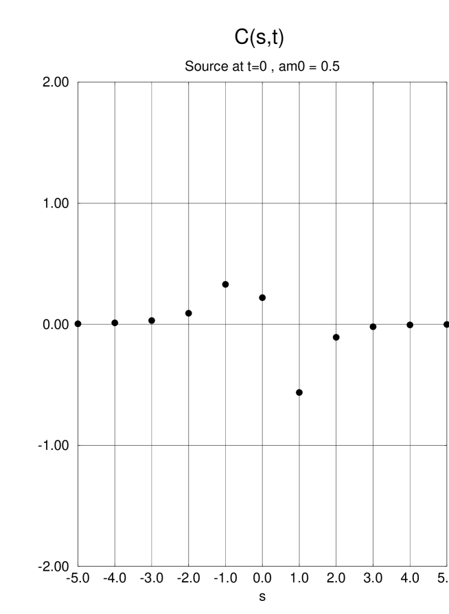
FIG. 9.: The coefficient of the anomaly $C(s,t)$ in 2+1 dimensions as a function of $s$ for $t=0$ fixed at $m_{0}=0.5$ and $L=5$.

REFERENCES

• [1] H. B. Nielsen and M. Ninomiya, Nucl. Phys. B185, 20 (1981); erratum: Nucl. Phys. B195, 541 (1982); Nucl. Phys. B193,173 (1981); Phys. Lett. 105B, 219 (1981).
• [2] L. H. Karsten, Phys. Lett. B104, 315 (1981).
• [3] D.B. Kaplan, Phys. Lett B288, 342 (1992).
• [4] K. Jansen, Phys. Lett. B288 348 (1992).
• [5] S. Aoki and H. Hirose, Phys. Rev. D49, 2604 (1994).
• [6] M.F.L. Golterman, K. Jansen and D.B. Kaplan, Phys. Lett. B301, 219 (1993).
• [7] D. Kaplan, Nucl. Phys. B (Proc.Suppl.) 30, 597 (1993).
• [8] T. Kawano and Y. Kikukawa, Phys. Rev. D50, 5365 (1994).
• [9] S. Chandrasekharan, Phys. Rev. D49, 1980 (1994).
• [10] S. Randjbar-Daemi and J. Strathdee, Nucl. Phys. B443, 386 (1995).
• [11] C.P. Korthals-Altes, S. Nicolis and J. Prades, Phys. Lett. B316, 339 (1993).
• [12] H. Aoki, S. Ito, J. Nishimura and M. Oshikawa, Mod. Phys. Lett.  A9, 1755 (1994).
• [13] S. Aoki and K. Nagai, “Domain-wall fermions with $U(1)$ dynamical gauge fields”, Univ. of Tsukuba preprint, UTHEP-314.
• [14] S. Aoki and R. B. Levien, Phys. Rev.  D51, 3790 (1995).
• [15] Y. Shamir, Nucl. Phys. B406, 90 (1993); Nucl. Phys. B417,167 (1993); Phys. Lett. B305, 357 (1992).
• [16] M.F.L. Golterman, K. Jansen, D.N. Petcher and J. Vink, Phys. Rev. D49, 1606 (1994).
• [17] M.F.L. Golterman and Y. Shamir, Phys. Rev. D51, 3026 (1995).
• [18] R. Narayanan and H. Neuberger, Phys. Lett. B302, 62 (1993); Phys. Rev. Lett. 71, 3251 (1993); Nucl. Phys. B412, 574 (1994); Nucl. Phys. B (Proc. Suppl.) 34, 587 (1994).
• [19] R. Narayanan, Nucl. Phys. B (Proc.Suppl.) 34, 95 (1994).
• [20] M.F.L. Golterman and Y. Shamir, Phys. Lett. B353, 84 (1995) .
• [21] J. Distler and S.-J. Rey, “3 into 2 doesn’t go”, Princeton preprint, PUPT-1386.
• [22] H. Kawai, R. Nakayama and K. Seo, Nucl. Phys. B190, 40 (1981).
• [23] S. Aoki, Phys. Rev Lett.  60, 2109 (1988); Phys. Rev. D38, 618 (1988).