Molecular dynamics for full QCD simulations with an improved action

Abstract

I derive the equation of motion in molecular dynamics for doing full lattice QCD simulations with clover quarks. The even-odd preconditioning technique, expected to significantly reduce the computational effort, is further developed for the simulations.

Published in Computer Physics Communications 94 (1996) 119-127.

1 Introduction

The effects of dynamical quarks are important in QCD at finite temperature as well as in some phenomenological aspects at zero temperature. Unfortunately, the inclusion of dynamical quarks is the most demanding task in computer simulations of lattice QCD. The hybrid molecular dynamics or Hybrid Monte Carlo (HMC) methods have been developed into very efficient algorithms (maybe the most popular) for dynamical quarks. In these algorithms, the equation of motion is the essential ingredient. One has to derive the relevant equations before writing the programs for molecular dynamical simulations. For lattice QCD with staggered or Wilson fermions, these equations have already been available in the literature [1, 2, 3].

Lattice QCD has discretization errors due to the lattice spacing $a$. At intermediate bare coupling, corresponding to relatively large $a$, these systematic errors might sometimes be very severe for Wilson fermions due to the chiral symmetry breaking term. The current computers do not allow the calculations done for very small $a$, because to reduce $a$ implies to use a much larger lattice. Another way out is to use the improved fermionic actions. Recently, it has been shown that the use of the clover action [4, 5] can significantly reduce these finite cut-off errors. However, the calculations of the clover action are much more complicated than the standard Wilson action. To my knowledge, there has not been a simulation of lattice QCD with the clover action in the literature.

The purpose of this paper is to derive the equation of motion for full QCD simulations with the clover action. Because the fermionic matrix has to be inverted in each step of the molecular dynamics step, it is also challenging to devise efficient algorithms for preconditioning [2, 6] the fermionic matrix so that the inverse is easier to compute. For this reason, I also extend the even-odd preconditioning technique, previously used for quark propagator measurements, to the case of dynamical clover fermions.

2 Preconditioning

2.1 The action

The action of the theory is $S=S_{G}+S_{F}$, where

$$S_{G}=-{\beta\over N_{c}}\sum_{p}Re~{}tr(U_{p})$$

$$=-{\beta\over N_{c}}\sum_{x,\mu>\nu}Re~{}tr[U_{\mu}(x)U_{\nu}(x+\mu)U_{\mu}(x+\nu)^{\dagger}U_{\nu}(x)^{\dagger}]$$ (1)

is the gauge action. The clover action for the quarks [4, 5] is

$$S_{F}=\sum_{x,y}{\bar{\psi}}(x)M_{xy}\psi(y)=\sum_{x,y}{\bar{\psi}}(x)(A_{x,y}-\kappa B_{x,y})\psi(y),$$

$$A_{x,y}=\delta_{x,y}[1-{\kappa C\over 2}\sum_{\mu,\nu}\sigma_{\mu\nu}{\mathcal{F}_{\mu\nu}}(x)],$$

$$B_{x,y}=\sum_{\mu=1}^{4}(1-\gamma_{\mu})U_{\mu}(x)\delta_{x,y-\mu}+(1+\gamma_{\mu})U^{\dagger}_{\mu}(x-\mu)\delta_{x,y+\mu}.$$ (2)

$A$ is local and hermitian, and $B$ connects only the nearest neighbor sites. The field strength tensor on the lattice is defined by ${\mathcal{F}_{\mu\nu}}(x)=[Q_{\mu\nu}(x)-Q_{\mu\nu}^{\dagger}(x)]/2i$, where $Q_{\mu\nu}$ is the averaged sum of four plaquettes on the $\mu\nu$ plane with the lattice site $x$ as one corner. Each plaquette is the product of four link variables in the counterclockwise sense and begins with the link variable directed away from the site $x$ and ends with the link variable directed towards site $x$, i.e.,

$$Q_{\mu\nu}(x)={1\over 4}[U_{\mu}(x)U_{\nu}(x+\mu)U_{\mu}(x+\nu)^{\dagger}U_{\nu}(x)^{\dagger}$$

$$+U_{\nu}(x)U_{\mu}(x-\mu+\nu)^{\dagger}U_{\nu}(x-\mu)^{\dagger}U_{\mu}(x-\mu)$$

$$+U_{\mu}(x-\mu)^{\dagger}U_{\nu}(x-\mu-\nu)^{\dagger}U_{\mu}(x-\mu-\nu)U_{\nu}(x-\nu)$$

$$+U_{\nu}(x-\nu)^{\dagger}U_{\mu}(x-\nu)U_{\nu}(x+\mu-\nu)U_{\mu}(x)^{\dagger}]$$ (3)

as shown in Fig. 1. This operator is so chosen as for the maximal symmetry on the lattice. Most symbols in above equations are conventional, while the coefficient $C$ in (2) depends on the choice of improvement strategy: $C=1$ for tree level improvement, and $C=[Re~{}tr(U_{p})/N_{c}]^{-3/4}$ for the tadpole improvement [7].

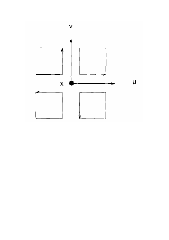
Figure 1: Plot of the clover operator $Q_{\mu\nu}$. The product in the plaquette is in counterclockwise sense and begins with the directed link.

2.2 Even-odd splitting

The lattice sites can be organized in an even-odd checkerboard and the even sites are numbered before the odd sites such that the fermionic matrix can be written as [8, 9]

$$M=\left(\begin{array}[]{cc}A_{ee}&-\kappa B_{eo}\\ -\kappa B_{oe}&A_{oo}\end{array}\right),$$ (6)

where $e$ or $o$ denotes even or odd site on the lattice.

Using such an arrangement, we obtain

$$\det(M)=\det(A_{oo})~{}\det(A_{ee}-\kappa^{2}B_{eo}A^{-1}_{oo}B_{oe})=\det A_{oo}~{}\det M_{ee}$$ (7)

where

$$M_{ee}=A_{ee}-\kappa^{2}B_{eo}A^{-1}_{oo}B_{oe},$$ (8)

which couples only to even sites of the lattice. Now $\det(M)$ on the whole lattice has been factorized as a product of the determinant of the local matrix $A$ on the odd lattice and that of $M_{ee}$ on the even lattice.

To calculate the fermionic determinant, it is useful to introduce the pseudo-scalar variables $\eta_{o}$ and $\phi_{e}$, so that

$$\det(M^{\dagger}M)=\det(A^{\dagger}_{oo}A_{oo})~{}\det(M^{\dagger}_{ee}M_{ee})=\int d\eta_{o}^{\dagger}~{}d\eta_{o}\int d\phi_{e}^{\dagger}~{}d\phi_{e}exp(-S_{pf})$$

$$=\int d\eta_{o}^{\dagger}~{}d\eta_{o}~{}exp[-\eta_{o}^{\dagger}(A^{\dagger}_{oo}A_{oo})^{-1}\eta_{o}]\int d\phi_{e}^{\dagger}~{}d\phi_{e}~{}exp[-\phi_{e}^{\dagger}(M^{\dagger}_{ee}M_{ee})^{-1}\phi_{e}],$$ (9)

where $S_{pf}$ is the pseudo-fermionic action

$$S_{pf}=\ \eta_{o}^{\dagger}(A^{\dagger}_{oo}A_{oo})^{-1}\eta_{o}+\phi_{e}^{\dagger}(M^{\dagger}_{ee}M_{ee})^{-1}\phi_{e},$$ (10)

describing two flavor quarks with the same bare mass. Notice that $\eta_{o}=A^{\dagger}_{oo}\xi_{o}$ and $\phi_{e}=M^{\dagger}_{ee}\theta_{e}$ have no direct coupling, where $\xi_{o}$ and $\theta_{e}$ are Gaussian noises injected at beginning of each molecular dynamics trajectory and held fixed during each trajectory.

In the remaining text, I will use the above even-odd preconditioning to discuss the molecular dynamics.

2.3 Fermionic inversion

For quark propagator measurements and also in each molecular dynamics step, one has to calculate $M_{ee}^{-1}$ or $(M^{\dagger}_{ee}M_{ee})^{-1}$, which can be implemented using the standard techniques like minimum residue, conjugate gradient or stabilized biconjugate gradient algorithms. The advantage of the even-odd splitting, as can also be seen later, is that such inversion is implemented only on the even lattice. Furthermore, due to the factor $\kappa^{2}$ in (8), $M_{ee}$ is better conditioned than $M$.

For the inversion $A_{oo}^{-1}$ on each odd site, because it is completely local, we can use the $LDL^{\dagger}$ decomposition [9, 10] to solve it. Since it is a hermitian matrix, there exists a diagonal matrix $D$ and lower-triangular matrix $L$ such that $A=LDL^{\dagger}$. Denoting $i$ and $j$ as the color-spin indexes of $A$, then

$$D_{i}=A_{ii}-\sum_{k=1}^{i-1}L_{ik}D_{k}L^{\ast}_{ik},~{}~{}$$

$$L_{ij}D_{j}=A_{ij}-\sum_{k=1}^{j-1}L_{ik}D_{k}L^{\ast}_{jk},~{}~{}(j=1,...,i-1).$$ (11)

We can also compute the solution of $AX=b$ by $y=L^{-1}b$ and $X=(L^{\dagger})^{-1}D^{-1}Y$, i.e.,

$$Y_{i}=b_{i}-\sum_{k=1}^{i-1}L_{ik}Y_{k},~{}~{}(i=1,...,n),~{}~{}$$

$$X_{i}=Y_{i}/D_{i}-\sum_{k=i+1}^{n}L_{ki}^{\ast}X_{k},~{}~{}(i=n,...,1),$$ (12)

with $n=12$, which is the number of colors times the number of spins. The calculation is quite easy because there are $n^{2}$ multiplications and only $n$ divisions.

3 Molecular dynamics

3.1 Equation of motion

To develop the equation of motion for the gauge field ${\mathcal{A}_{\mu}}(x)$, one has to introduce a Hamiltonian $H=\sum_{x,\mu}P^{2}_{{\mathcal{A}_{\mu}}(x)}/2+S_{g}+S_{pf}$, with $P_{{\mathcal{A}_{\mu}}(x)}$ the canonical conjugate momentum defined by $P_{{\mathcal{A}_{\mu}}(x)}=\partial H/\partial(d{\mathcal{A}_{\mu}}(x)/d\tau)$, and $\tau$ being the fictious molecular dynamics time.

The gauge configurations are generated by solving the Hamiltonian equation of motion:

$${d{\mathcal{A}_{\mu}}(x)\over d\tau}=P_{{\mathcal{A}_{\mu}}(x)},~{}~{}{dP_{{\mathcal{A}_{\mu}}(x)}\over d\tau}={\partial H\over\partial{\mathcal{A}_{\mu}}(x)}=-{\partial S_{G}\over\partial{\mathcal{A}_{\mu}}(x)}-{\partial S_{pf}\over\partial{\mathcal{A}_{\mu}}(x)}.$$ (13)

For the gauge action, it is quite easy to show that

$$-{\partial S_{G}\over\partial{\mathcal{A}_{\mu}}(x)}={\beta\over 2N_{c}}[{\partial U_{\mu}(x)\over\partial{\mathcal{A}_{\mu}}(x)}STAPLE_{\mu}(x)+STAPLE_{\mu}(x)^{\dagger}{\partial U_{\mu}(x)^{\dagger}\over\partial{\mathcal{A}_{\mu}}(x)}]$$

$$={i\beta\over 2N_{c}}[U_{\mu}(x)STAPLE_{\mu}(x)-h.c.],$$ (14)

where $STAPLE_{\mu}(x)$ is the sum over six staples surrounding the link $U_{\mu}(x)$. For the fermionic part,

$$-{\partial S_{pf}\over\partial{\mathcal{A}_{\mu}}(x)}=X_{o}^{A\dagger}{\partial(A^{\dagger}_{oo}A_{oo})\over\partial{\mathcal{A}_{\mu}}(x)}X_{o}^{A}+X_{e}^{\dagger}{\partial(M^{\dagger}_{ee}M_{ee})\over\partial{\mathcal{A}_{\mu}}(x)}X_{e},$$ (15)

where

$$X_{o}^{A}=(A^{\dagger}_{oo}A_{oo})^{-1}\eta_{o},~{}~{}X_{e}=(M^{\dagger}_{ee}M_{ee})^{-1}\phi_{e}.$$ (16)

If we define two more variables

$$Y_{o}^{A}=A_{oo}X_{o}^{A},~{}~{}Y_{e}=M_{ee}X_{e},$$ (17)

(15) can be simply rewritten as

$$-{\partial S_{pf}\over\partial{\mathcal{A}_{\mu}}(x)}=X_{o}^{A\dagger}{\partial A^{\dagger}_{oo}\over\partial{\mathcal{A}_{\mu}}(x)}Y_{o}^{A}+Y_{o}^{A\dagger}{\partial A_{oo}\over\partial{\mathcal{A}_{\mu}}(x)}X_{o}^{A}$$

$$+X_{e}^{\dagger}{\partial M^{\dagger}_{ee}\over\partial{\mathcal{A}_{\mu}}(x)}Y_{e}+Y_{e}^{\dagger}{\partial M_{ee}\over\partial{\mathcal{A}_{\mu}}(x)}X_{e}.$$ (18)

A straightforward computation leads to

$${\partial M_{ee}\over\partial{\mathcal{A}_{\mu}}(x)}={\partial A_{ee}\over\partial{\mathcal{A}_{\mu}}(x)}-\kappa^{2}{\partial B_{eo}\over\partial{\mathcal{A}_{\mu}}(x)}A_{oo}^{-1}B_{oe}$$

$$+\kappa^{2}B_{eo}A_{oo}^{-1}{\partial A_{oo}\over\partial{\mathcal{A}_{\mu}}(x)}A_{oo}^{-1}B_{oe}-\kappa^{2}B_{oe}A_{oo}^{-1}{\partial B_{oe}\over\partial{\mathcal{A}_{\mu}}(x)},$$

$${\partial M^{\dagger}_{ee}\over\partial{\mathcal{A}_{\mu}}(x)}={\partial A_{ee}\over\partial{\mathcal{A}_{\mu}}(x)}-\kappa^{2}{\partial B^{\dagger}_{eo}\over\partial{\mathcal{A}_{\mu}}(x)}A_{oo}^{-1}B^{\dagger}_{oe}$$

$$+\kappa^{2}B^{\dagger}_{eo}A_{oo}^{-1}{\partial A_{oo}\over\partial{\mathcal{A}_{\mu}}(x)}A_{oo}^{-1}B^{\dagger}_{oe}-\kappa^{2}B^{\dagger}_{oe}A_{oo}^{-1}{\partial B^{\dagger}_{oe}\over\partial{\mathcal{A}_{\mu}}(x)}.$$ (19)

By defining the following variables on the odd sites

$$X_{o}=\kappa A_{oo}^{-1}B_{oe}X_{e},~{}~{}Y_{o}=\kappa A_{oo}^{-1}B_{oe}^{\dagger}Y_{e},$$ (20)

we have

$$Y_{e}^{\dagger}{\partial M_{ee}\over\partial{\mathcal{A}_{\mu}}(x)}X_{e}=Y_{e}^{\dagger}{\partial A_{ee}\over\partial{\mathcal{A}_{\mu}}(x)}X_{e}+Y_{o}^{\dagger}{\partial A_{oo}\over\partial{\mathcal{A}_{\mu}}(x)}X_{o}$$

$$-\kappa Y_{e}^{\dagger}{\partial B_{eo}\over\partial{\mathcal{A}_{\mu}}(x)}X_{o}-\kappa Y_{o}^{\dagger}{\partial B_{oe}\over\partial{\mathcal{A}_{\mu}}(x)}X_{e},$$

$$X_{e}^{\dagger}{\partial M_{ee}^{\dagger}\over\partial{\mathcal{A}_{\mu}}(x)}Y_{e}=X_{e}^{\dagger}{\partial A_{ee}\over\partial{\mathcal{A}_{\mu}}(x)}Y_{e}+X_{o}^{\dagger}{\partial A_{oo}\over\partial{\mathcal{A}_{\mu}}(x)}Y_{o}$$

$$-\kappa X_{e}^{\dagger}{\partial B^{\dagger}_{eo}\over\partial{\mathcal{A}_{\mu}}(x)}Y_{o}-\kappa X_{o}^{\dagger}{\partial B^{\dagger}_{oe}\over\partial{\mathcal{A}_{\mu}}(x)}Y_{e}.$$ (21)

We can further demonstrate that the last two terms of these two equations in (21) are summarized as

$$-\kappa Y_{e}^{\dagger}{\partial B_{eo}\over\partial{\mathcal{A}_{\mu}}(x)}X_{o}-\kappa Y_{o}^{\dagger}{\partial B_{oe}\over\partial{\mathcal{A}_{\mu}}(x)}X_{e}-\kappa X_{e}^{\dagger}{\partial B^{\dagger}_{eo}\over\partial{\mathcal{A}_{\mu}}(x)}Y_{o}-\kappa X_{o}^{\dagger}{\partial B^{\dagger}_{oe}\over\partial{\mathcal{A}_{\mu}}(x)}Y_{e}$$

$$=-\kappa\sum_{x^{\prime},y}[Y_{x^{\prime}}^{\dagger}{\partial B_{x^{\prime}y}\over\partial{\mathcal{A}_{\mu}}(x)}X_{y}+X_{x^{\prime}}^{\dagger}{\partial B^{\dagger}_{x^{\prime}y}\over\partial{\mathcal{A}_{\mu}}(x)}Y_{y}]=-i\kappa[U_{\mu}(x)F_{\mu}^{W}-h.c.],$$ (22)

where

$$F_{\mu}^{W}=tr_{dirac}[(1+\gamma_{\mu})Y_{x+\mu}X_{x}^{\dagger}+(1-\gamma_{\mu})X_{x+\mu}Y_{x}^{\dagger}],$$ (23)

the same form as the fermionic force in the Wilson fermion case. As can also be seen later, the last two terms in (18) have exactly the same form for even and odd sites. Therefore, the introduction of the variables (16), (17) and (20) has a great advantage.

A remark has to be made: to keep the conjugate momentum traceless, the right hand side (r.h.s.) of (13) should finally be subtracted by a term being the trace of the r.h.s. divided by $N_{c}$.

3.2 Practical implementation

The simulations should be carried out in the first two steps as follows.

1) Generating the full configurations. In numerical integration of the equation of motion, one has to Taylor expand $U(\tau+d\tau)=exp[id\tau P(\tau)]U(\tau)=U(\tau)+id\tau P(\tau)U(\tau)+...$, $P(\tau+d\tau)=P(\tau)+d\tau{dP\over d\tau}(\tau)+...$, with finite order truncation. The leapfrog scheme can reduce the truncation errors to $N_{md}O(d\tau^{3})=O(d\tau^{2})$ at $N_{md}$ molecular dynamical steps. These errors can be canceled by a Metropolis test at the end of the trajectory. Of course, this $d\tau$ has to be fine tuned to maintain high acceptance rate and small auto-correlation time.

2) About the clover coefficient. For the tree level improvement, $C=1$. For the tadpole improvement scheme, the value of $C$ depends dynamically on the configurations. One has to determine $C$ self-consistently from the simulation. For example, one may first have an initial guess for it, then generate a gauge configuration. From the plaquette, we can get a new $C$ value. After some iteration, $C$ might converge to some stable value for some given $\beta$ and $\kappa$. (This could be done very quickly since the plaquette can be accurately measured with a small number of configurations and on small lattices, provided the system is far away from a phase transition).

3) Measuring the physical quantities. To obtain the improved hadronic matrix elements, rotation of quark fields [5, 8] is necessary.

4 More details about the fermionic force

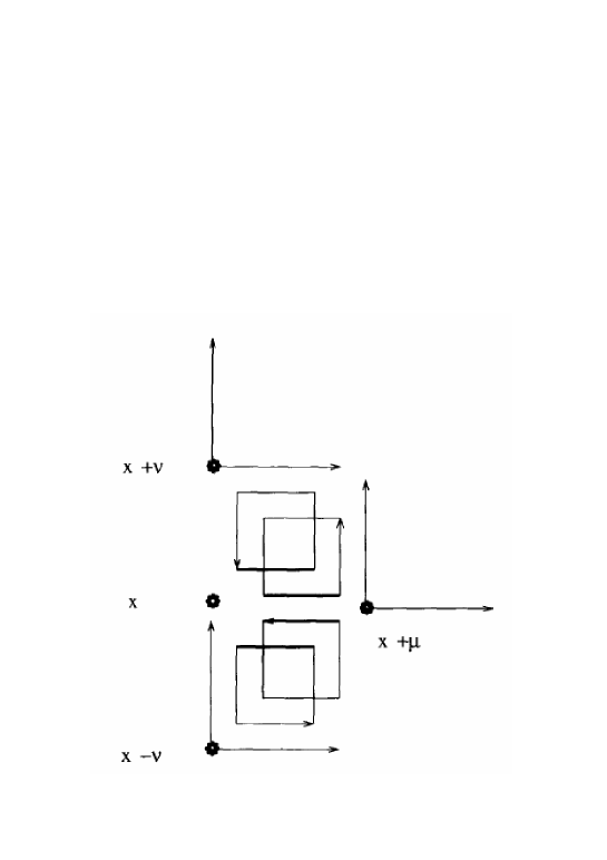
Figure 2: Relevant plaquettes for $\sum_{y}[Y_{y}^{A\dagger}(\partial A_{yy}/\partial{\mathcal{A}_{\mu}}(x))X_{y}^{A}+X_{y}^{A\dagger}(\partial A^{\dagger}_{yy}/\partial{\mathcal{A}_{\mu}}(x))Y_{y}^{A}]$ when $x\in y$, where the thick lines indicate the links relevant for $\partial U_{\mu}(x)/{\partial\mathcal{A}_{\mu}}(x)$ or $\partial U_{\mu}(x)^{\dagger}/{\partial\mathcal{A}_{\mu}}(x)$.

I have described that how the introduction of the variables (16), (17) and (20) leads to the equation of motion similar to that of the Wilson case. What is different is the terms with matrix $A$, which makes the equation of motion much more complicate. Therefore, it deserves further discussions. Note the term in the pseudo-fermion action $Y_{o}^{A\dagger}A_{oo}X_{o}^{A}$ (also the second term) is placed only on odd sites of the lattice, then for $x$ being odd sites, there are terms only on $x$, $x+\mu+\nu$ and $x+\mu-\nu$ relevant for $Y_{o}^{A\dagger}(\partial A_{oo}/\partial{\mathcal{A}_{\mu}}(x))X_{o}^{A}$ as shown in Fig. 2, i.e.,

$${1\over 2}Y_{o}^{A\dagger}\sum_{\mu^{\prime}\not=\nu}\sigma_{\mu^{\prime}\nu}{\partial Q_{\mu^{\prime}\nu}(o)\over\partial{\mathcal{A}_{\mu}}(x)}X_{o}^{A}=$$

$${1\over 4}\sum_{\nu}~{}^{\prime}~{}Y_{x}^{A\dagger}\sigma_{\mu\nu}[{\partial U_{\mu}(x)\over{\partial\mathcal{A}_{\mu}}(x)}U_{\nu}(x+\mu)U_{\mu}(x+\nu)^{\dagger}U_{\nu}(x)^{\dagger}$$

$$+U_{\nu}(x-\nu)^{\dagger}U_{\mu}(x-\nu)U_{\nu}(x+\mu-\nu){\partial U_{\mu}(x)^{\dagger}\over{\partial\mathcal{A}_{\mu}}(x)}]X_{x}^{A}$$

$$+{1\over 4}\sum_{\nu}~{}^{\prime}~{}Y_{x+\mu+\nu}^{A\dagger}\sigma_{\mu\nu}U_{\mu}(x+\nu)^{\dagger}U_{\nu}(x)^{\dagger}{\partial U_{\mu}(x)\over{\partial\mathcal{A}_{\mu}}(x)}U_{\nu}(x+\mu)X_{x+\mu+\nu}^{A}$$

$$+{1\over 4}\sum_{\nu}~{}^{\prime}~{}Y_{x+\mu-\nu}^{A\dagger}\sigma_{\mu\nu}U_{\nu}(x+\mu-\nu){\partial U_{\mu}(x)^{\dagger}\over{\partial\mathcal{A}_{\mu}}(x)}U_{\nu}(x-\nu)^{\dagger}U_{\mu}(x-\nu)X_{x+\mu-\nu}^{A}.$$

(24)

Here $\sum_{\nu}^{\prime}$ means the sum over $\nu\neq\mu$. For $x$ being even sites, there are terms only on $x+\mu$, $x+\nu$ and $x-\nu$ as shown in Fig. 3, i.e.,

$${1\over 2}Y_{o}^{A\dagger}\sum_{\mu^{\prime}\not=\nu}\sigma_{\mu^{\prime}\nu}{\partial Q_{\mu^{\prime}\nu}(o)\over{\partial\mathcal{A}_{\mu}}(x)}X_{o}^{A}=$$

$${1\over 4}\sum_{\nu}~{}^{\prime}~{}Y_{x+\mu}^{A\dagger}\sigma_{\mu\nu}[U_{\nu}(x+\mu)U_{\mu}(x+\nu)^{\dagger}U_{\nu}(x)^{\dagger}{\partial U_{\mu}(x)\over{\partial\mathcal{A}_{\mu}}(x)}$$

$$+{\partial U_{\mu}(x)^{\dagger}\over{\partial\mathcal{A}_{\mu}}(x)}U_{\nu}(x-\nu)^{\dagger}U_{\mu}(x-\nu)U_{\nu}(x+\mu-\nu)]X_{x+\mu}^{A}$$

$$+{1\over 4}\sum_{\nu}~{}^{\prime}~{}Y_{x+\nu}^{A\dagger}\sigma_{\mu\nu}U_{\nu}(x)^{\dagger}{\partial U_{\mu}(x)\over{\partial\mathcal{A}_{\mu}}(x)}U_{\nu}(x+\mu)U_{\mu}(x+\nu)^{\dagger}X_{x+\nu}^{A}$$

$$+{1\over 4}\sum_{\nu}~{}^{\prime}~{}Y_{x-\nu}^{A\dagger}\sigma_{\mu\nu}U_{\mu}(x-\nu)U_{\nu}(x+\mu-\nu){\partial U_{\mu}(x)^{\dagger}\over{\partial\mathcal{A}_{\mu}}(x)}U_{\nu}(x-\nu)^{\dagger}X_{x-\nu}^{A}.$$

(25)

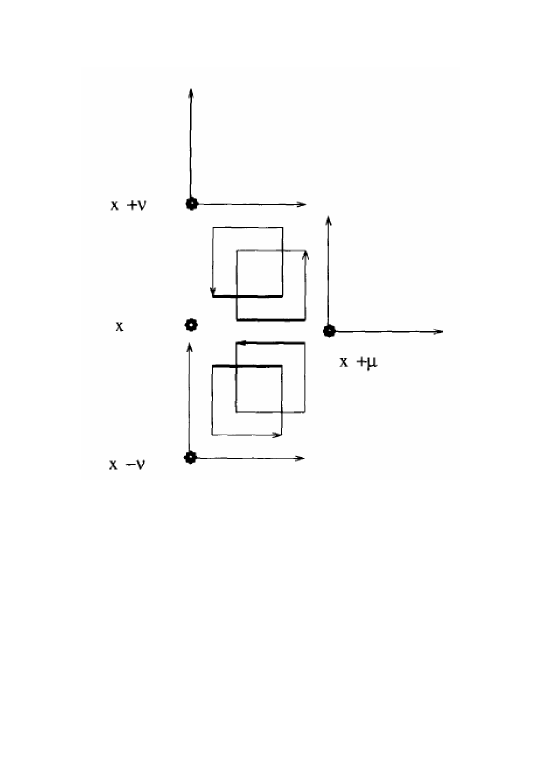
Figure 3: The same as Fig. 2 but for $x$ doesn’t belong to $y$.

Therefore for odd-site $x$, the first two terms in (18) read

$$Y_{o}^{A\dagger}{\partial A_{oo}\over{\partial\mathcal{A}_{\mu}}(x)}X_{o}^{A}+X_{o}^{A\dagger}{\partial A_{oo}^{\dagger}\over{\partial\mathcal{A}_{\mu}}(x)}Y_{o}^{A}=$$

$$-{\kappa C\over 8}[\sum_{\nu}~{}^{\prime}~{}Y_{x}^{A\dagger}\sigma_{\mu\nu}{\bf U_{\mu}(x)}U_{\nu}(x+\mu)U_{\mu}(x+\nu)^{\dagger}U_{\nu}(x)^{\dagger}X_{x}^{A}$$

$$-\sum_{\nu}~{}^{\prime}~{}Y_{x}^{A\dagger}\sigma_{\mu\nu}U_{\nu}(x-\nu)^{\dagger}U_{\mu}(x-\nu)U_{\nu}(x+\mu-\nu){\bf U_{\mu}(x)}^{\dagger}X_{x}^{A}$$

$$+\sum_{\nu}~{}^{\prime}~{}Y_{x+\mu+\nu}^{A\dagger}\sigma_{\mu\nu}U_{\mu}(x+\nu)^{\dagger}U_{\nu}(x)^{\dagger}{\bf U_{\mu}(x)}U_{\nu}(x+\mu)X_{x+\mu+\nu}^{A}$$

$$-\sum_{\nu}~{}^{\prime}~{}Y_{x+\mu-\nu}^{A\dagger}\sigma_{\mu\nu}U_{\nu}(x+\mu-\nu){\bf U_{\mu}(x)}^{\dagger}U_{\nu}(x-\nu)^{\dagger}U_{\mu}(x-\nu)X_{x+\mu-\nu}^{A}$$

$$+(Y\leftrightarrow X)+h.c.].$$ (26)

Similarly, for even $x$, the first two terms in (18) are

$$Y_{o}^{A\dagger}{\partial A_{oo}\over{\partial\mathcal{A}_{\mu}}(x)}X_{o}^{A}+X_{o}^{A\dagger}{\partial A_{oo}^{\dagger}\over{\partial\mathcal{A}_{\mu}}(x)}Y_{o}^{A}=$$

$$-{\kappa C\over 8}[\sum_{\nu}~{}^{\prime}~{}Y_{x+\mu}^{A\dagger}\sigma_{\mu\nu}U_{\nu}(x+\mu)U_{\mu}(x+\nu)^{\dagger}U_{\nu}(x)^{\dagger}{\bf U_{\mu}(x)}X_{x+\mu}^{A}$$

$$-\sum_{\nu}~{}^{\prime}~{}Y_{x+\mu}^{A\dagger}\sigma_{\mu\nu}{\bf U_{\mu}(x)}^{\dagger}U_{\nu}(x-\nu)^{\dagger}U_{\mu}(x-\nu)U_{\nu}(x+\mu-\nu)X_{x+\mu}^{A}$$

$$+\sum_{\nu}~{}^{\prime}~{}Y_{x+\nu}^{A\dagger}\sigma_{\mu\nu}U_{\nu}(x)^{\dagger}{\bf U_{\mu}(x)}U_{\nu}(x+\mu)U_{\mu}(x+\nu)^{\dagger}X_{x+\nu}^{A}$$

$$-\sum_{\nu}~{}^{\prime}~{}Y_{x-\nu}^{A\dagger}\sigma_{\mu\nu}U_{\mu}(x-\nu)U_{\nu}(x+\mu-\nu){\bf U_{\mu}(x)}^{\dagger}U_{\nu}(x-\nu)^{\dagger}X_{x-\nu}^{A}$$

$$+(Y\leftrightarrow X)+h.c.].$$ (27)

Equations (26) and (27) can be generalized to terms with $y$ being odd or even:

$$\sum_{y}[Y_{y}^{\dagger}{\partial A_{yy}\over{\partial\mathcal{A}_{\mu}}(x)}X_{y}+X_{y}^{\dagger}{\partial A_{yy}^{\dagger}\over{\partial\mathcal{A}_{\mu}}(x)}Y_{y}]$$

$$=(\ref{DAO}),~{}~{}if~{}x\in y,$$

$$=(\ref{DAE}),~{}~{}if~{}x\notin y.$$ (28)

These relations are also quite useful when deriving the first two terms in (21).

Summarizing (22) and (28), (18) becomes

$$-{\partial S_{pf}\over\partial{\mathcal{A}_{\mu}}(x)}$$

$$=(\ref{DAE})+[(\ref{DAE})+(\ref{DAO})](X^{A}\to X,Y^{A}\to Y)+(\ref{DB}),~{}~{}if~{}x=even,$$

$$=(\ref{DAO})+[(\ref{DAE})+(\ref{DAO})](X^{A}\to X,Y^{A}\to Y)+(\ref{DB}),~{}~{}if~{}x=odd.$$ (29)

Note that the difference in the form of the molecular dynamics equation on even and odd sites is only in the first term.

5 Discussions

In this paper, I have derived (14) and (29), relevant for equation of motion (13) in molecular dynamics (or HMC) simulations with clover fermions. I have also extended the even-odd precondition technique, previously introduced for the quark propagator measurements, to the case of simulations with dynamical clover fermions. With the preconditioning technique, the number of iterations required would be reduced by a factor of $3$ according to experience, and the most expensive part of the fermionic inversion is performed only on half lattice size. Therefore, it is expected that the preconditioned equation of motion would lead to considerable improvement over the unpreconditioned one. This scheme is vectorizable and has been parallelized. Currently, the simulations of QCD at finite temperature using the clover action are being carrying out on the Quadrics-APE100 parallel computers. The above work might lay a foundation of further computer simulations using dynamical clover fermions.

Of course, to obtain physical results from the numerical simulations, there are still of lot of work to do. For instance, because the clover constant $C$ depends dynamically on the gauge configuration, then there would be delicate interplay between $C$ and $\beta$, $\kappa$, in particular when the system is at criticality. This is a new subject beyond the scope of the paper.

It has been mentioned in [8] that even for the quenched clover propagator calculations, each minimum residue iteration took $35\%$ longer than for the Wilson action. One has to choose a more efficient algorithm for fermionic inversion because a good algorithm is critical for full simulations. It is known that the stabilized biconjugate gradient is more efficient than the minimum residue or conjugate gradient, reducing the CPU time by at least a factor of 1.5.

Even if with the clover action there is an improvement of the finite cut-off error, the simulations with this action require larger statistical samples, more arithmetic operations and much memory. Concerning the feasibility of a full QCD clover simulation on supercomputers, it is not easy to quantify, because it is machine and code dependent.

I hope to discuss these problems and report the physical results in the near future.

References

[1] S. Gottlieb, W. Liu, D. Toussaint,
R. Renken, and R. Sugar,
Phys. Rev. D35 (1987) 2531.
[2] R. Gupta, A. Patel, C. Baillie,
G. Guralnik, G. Kilcup, and
S. Sharpe, Phys. Rev. D40 (1989) 2072.
[3]
S. Antonelli, M. Bellacci, A. Donini, R. Sarno, “Full QCD on APE100
machines”, hep-lat/9311002.
[4] S. Sheikholeslami
and R. Wohlert, Nucl. Phys. B259
(1985) 572.
[5] G. Heatlie, C. Sachrajda, G. Martinelli, C. Pittori
and G. Rossi, Nucl. Phys. B352 (1991) 266.
[6] T. Degrand and P. Rossi, Computer Phys. Commun. 60
(1990) 211.