Finite volume effects and quenched chiral logarithms

Abstract

We have measured the valence pion mass and the valence chiral condensate on lattice configurations generated with and without dynamical fermions. We find that our data and that of others is well represented by a linear relationship between $m_{\pi}^{2}$ and the valence quark mass, with a non-zero intercept. For our data, we relate the intercept to finite volume effects visible in the valence chiral condensate. We see no evidence for the singular behavior expected from quenched chiral logarithms.

1 INTRODUCTION

Over the last few years, analytic calculations using chiral perturbation theory have indicated pathologies in the quenched approximation [1, 2]. One example is the lack of closed quark loops contributing to propagation of the quenched $\eta^{\prime}$, which leads to a double pole in the quenched $\eta^{\prime}$ propagator. This leads to the following singular behavior for the valence pion mass [2]:

$$m_{\pi}^{2}=(2\mu m)^{\frac{1}{1+\delta}}\left(\Lambda^{2}\right)^{\frac{\delta}{1+\delta}}$$ (1)

For lattice calculations, there is some uncertainty about the mass $m$ to be used in the above. Due to the flavor symmetry breaking of staggered fermions at finite lattice spacing, the pions are not degenerate in mass in current simulations and the quenched $\eta^{\prime}$ may be closer in mass to the heavier pions than the lighter ones. Interpreting the $m$ above as the bare quark mass assumes the $\eta^{\prime}$ is closer in mass to the lightest, Goldstone boson, pion [3].

Another consequence of the chiral perturbation theory calculations is the absence of quenched chiral logarithms in decay constants, in particular in $f_{\pi}$. Because there is a lattice version of the Gell-Mann–Oakes–Renner (GMO) relation, this means that quenched chiral logarithms in the pion mass must be compensated by quenched chiral logarithms in the quenched chiral condensate.

Recently, there have been reports of simulation data consistent with the presence of quenched chiral logarithms, particularly in $m_{\pi}$ [4, 5]. To assess whether the data clearly reveals quenched chiral logarithms, we have investigated three points:

1. What effects do dynamical fermions have on the data? Does the signal persist and is it suppressed by the dynamical fermion mass?

2. Are quenched chiral logarithms evident in the valence chiral condensate?

3. Have all finite volume effects been clearly controlled?

This note will detail some of our results from the pursuit of these questions.

2 RELATING $m_{\pi}^{2}$ and $\langle\bar{\zeta}\zeta\rangle$

Since we will be referring to both quenched and dynamical simulations, we will introduce a species of staggered fermion, denoted by $\zeta$, which does not appear in the action. This valence fermion of mass $m_{\zeta}$ will be used to construct the valence pion propagators and the valence chiral condensate. The mass of the fermions entering the determinant will be denoted by $m$.

Consider an operator $\pi(x)$ which creates a pion. We can define a function $C(m_{\zeta})$ by

$$C(m_{\zeta})=m_{\pi}^{2}(m_{\zeta})\,\int\,d^{4}x\,\langle\pi(x)\pi(0)\rangle$$ (2)

The angle brackets can represent averaging over any ensemble of gauge fields, quenched or dynamical. Provided the volume is large enough and $m_{\pi}$ is much less than the mass of any other state with the same quantum numbers, $m_{\pi}$ in this relation is the mass determining the decay of the pion propagator.

We now rewrite equation (2) using the eigenvalues, $\lambda$, and the density of eigenvalues per unit volume in a background configuration $U$, $\rho(\lambda,U)$, of the staggered fermion Dirac operator, $D(U)$. We choose our conventions such that $D\,\zeta_{\lambda}(x)=i\,\lambda\,\zeta_{\lambda}(x)$ and $\int\,d\lambda\,\rho(\lambda,U)=1$. Using the U(1) symmetry of staggered fermions, we find that the eigenvalues come in pairs, $\pm\lambda$, and

$$\int\;d^{4}x\;\langle\pi(x)\pi(0)\rangle=2\int_{0}^{\infty}\;d\lambda\;\frac{\bar{\rho}(\lambda,\beta,m)}{\lambda^{2}+m_{\zeta}^{2}}$$ (3)

where $\bar{\rho}(\lambda,\beta,m)$ is the ensemble average of $\rho(\lambda,U)$.

We can also write the valence chiral condensate in terms of the eigenvalue density as

$$\langle\bar{\zeta}\zeta(m_{\zeta})\rangle=2m_{\zeta}\int_{0}^{\infty}\;d\lambda\;\frac{\bar{\rho}(\lambda,\beta,m)}{\lambda^{2}+m_{\zeta}^{2}}$$ (4)

We therefore have the relation

$$C(m_{\zeta})=\frac{m_{\pi}^{2}(m_{\zeta})\;\langle\bar{\zeta}\zeta(m_{\zeta})\rangle}{m_{\zeta}}$$ (5)

If $C(m_{\zeta})$ is known from either simulations or analytic arguments, this equation connects $m_{\pi}^{2}$ and $\langle\bar{\zeta}\zeta(m_{\zeta})\rangle$ including any effects of finite volume or quenched chiral logarithms.

We now focus on equation (4) and make a simple model for the effects of finite volume. In the continuum, chiral symmetry breaking is associated with a non-zero value for $\bar{\rho}(0)$, since $\langle\bar{\zeta}\zeta(0)\rangle=2\pi\bar{\rho}(0)$. The major effect of finite volume can be postulated to be a minimum eigenvalue, $\lambda_{\rm min}$, below which the average density of eigenvalues vanishes. In particular, consider $\bar{\rho}(\lambda)$ of the form

$$\bar{\rho}(\lambda)=\left\{\begin{array}[]{ll}0&\lambda<\lambda_{\rm\min}\\ \rho_{0}&\lambda_{\rm min}<\lambda<\lambda_{0}\\ \int_{\lambda_{0}}^{\infty}\;\rho(\lambda)\;d\lambda=\alpha&\lambda_{0}<\lambda\end{array}\right.$$ (6)

where $\alpha$ diverges in the continuum limit due to the quadratic divergences in $\langle\bar{\zeta}\zeta(m_{\zeta})\rangle$. Integrating equation (4) for our model gives, for $\lambda_{\rm min}<m_{\zeta}<\lambda_{0}$,

$$\langle\bar{\zeta}\zeta(m_{\zeta})\rangle=\rho_{0}\left[\frac{\pi}{2}-\frac{\lambda_{\rm min}}{m_{\zeta}}+m_{\zeta}(\alpha-\frac{1}{\lambda_{0}})\right]$$ (7)

plus terms of $O(m_{\zeta}^{2})$ and $O(1/m_{\zeta}^{2})$. The model shows that $1/m_{\zeta}$ dependence in $\langle\bar{\zeta}\zeta(m_{\zeta})\rangle$ can be easily associated with finite volume effects.

3 RESULTS FOR $m_{\pi}^{2}$ and $\langle\bar{\zeta}\zeta(m_{\zeta})\rangle$

We will be comparing the results from four staggered simulations, two quenched and two unquenched. Figure 1 shows $m_{\pi}^{2}$ versus $m_{\zeta}$ for these four simulations as well as the simulation parameters. The $32^{3}\times 64$ quenched simulation is the work of Kim and Sinclair [4]; the rest were done at Columbia. The rise for small $m_{\zeta}$ is the type of behavior expected from equation (1). Unfortunately, this kind of rise has been evident for some time in simulations and has been widely attributed to finite volume effects. In Figure 2 we replot the data, this time without dividing by $m_{\zeta}$. The data is well fit by a straight line, with a non-zero intercept.

Figure 1: $m_{\pi}^{2}/m_{\zeta}$ versus $m_{\zeta}$.

Figure 2: $m_{\pi}^{2}$ versus $m_{\zeta}$.

The correlated data column of Table 1 gives a list of the fit parameters we have obtained for fits to $m_{\pi}^{2}$, without the covariance matrix, of the form

$$m_{\pi}^{2}=c_{0}+c_{1}m_{\zeta}$$ (8)

Of course, one should use the full covariance matrix while fitting. We have tried single-elimination jackknife fits which simultaneously fit $m_{\pi}$ for all values of $m_{\zeta}$ and an appropriate range of times, but we have found such fits to be quite unstable given the large dimensionality of the covariance matrix. Instead we have decorrelated our data. In particular, we have broken our simulations into three or four smaller, equal length bins, determined $m_{\pi}$ for the lightest $m_{\zeta}$ from the first bin, for the next lightest from the second bin, etc. and then done an uncorrelated fit of the form given in equation (8). The results are given in the column labeled uncorrelated data in Table 1.

Table 1: Parameters for linear fits of $m_{\pi}^{2}$ versus $m_{\zeta}$.

		Correlated data			Uncorrelated data
$\beta$	$ma$	$c_{0}\times 10^{-3}$	$c_{1}$	$\chi^{2}$/dof	$c_{0}\times 10^{-3}$	$c_{1}$	$\chi^{2}$/dof
5.7	$\infty$	0.46(21)	8.32(5)	4.5/3	0.92(32)	8.24(7)	4.2/2
6.0	$\infty$	1.1(1)	5.69(2)	4.1/1
5.48	0.004	2.7(8)	8.27(12)	0.7/1	4.2(8)	8.01(12)	1.3/1
5.7	0.01	5.5(10)	5.59(12)	0.001/2	4.2(14)	5.69(14)	0.3/1

We now turn our attention to $\langle\bar{\zeta}\zeta(m_{\zeta})\rangle$. Figure 3 is a plot of the valence chiral condensate for the four simulations we are considering. Notice the log-log scale and the many orders of magnitude of $m_{\zeta}$ spanned by the Columbia simulations.

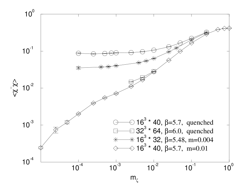
Figure 3: $\langle\bar{\zeta}\zeta(m_{\zeta})\rangle$ versus $m_{\zeta}$. The lines on the graph just connect the points. The $32^{3}\times 64$ data has been scaled to the Columbia normalization.

Figure 4 shows $\langle\bar{\zeta}\zeta(m_{\zeta})\rangle$ for the $\beta=5.7$, $ma=0.01$ simulation, on a linear plot. The line on the graph is a fit of the form

$$\langle\bar{\zeta}\zeta(m_{\zeta})\rangle=a_{0}+a_{1}m_{\zeta}-a_{-1}/m_{\zeta},$$ (9)

motivated by our simple model and equation (7). For the correlated fit shown, we find $a_{0}=0.0063(3)$, $a_{1}=2.13(1)$, $a_{-1}=8.9(5)\times 10^{-7}$ and $\chi^{2}/{\rm dof}=39(16)/2$. The value of $\chi^{2}$ is quite large, but the jackknifed error on it is also large. This generally indicates a poorly resolved small eigenvalue in the covariance matrix. An uncorrelated fit to the data gives $a_{0}=0.0061(3)$, $a_{1}=2.15(2)$, $a_{-1}=-8.8(8)\times 10^{-7}$ and $\chi^{2}/{\rm dof}=0.8/2$. Thus we have clear evidence for finite volume effects in $\langle\bar{\zeta}\zeta(m_{\zeta})\rangle$ and they are in agreement with the expectations of our simple model.

Figure 4: $\langle\bar{\zeta}\zeta(m_{\zeta})\rangle$ versus $m_{\zeta}$ for the $\beta=5.7$, $ma=0.01$ simulation.

4 INTERCEPT FOR $m_{\pi}^{2}$

We can now use equation (5) to give us an understanding of the origin of the non-zero intercept, $c_{0}$, found in fitting $m_{\pi}^{2}$. Assume that $C(m_{\zeta})$ is a non-singular function in the range $\lambda_{\rm min}<m_{\zeta}<\lambda_{0}$. Then, using the parameterization of equation (9) gives

$$m_{\pi}^{2}=-\frac{C(0)a_{-1}}{a_{0}^{2}}+\left[\frac{C(0)}{a_{0}}-\frac{C^{\prime}(0)a_{-1}}{a_{0}^{2}}\right]m_{\zeta}$$ (10)

plus terms of $O(m_{\zeta}^{2})$ and $O(1/m_{\zeta}^{2})$. This expansion is only valid in the range where $m_{\zeta}>\lambda_{\rm min}$, which is where most of our data lies. The non-zero intercept for $m_{\pi}^{2}$ is easily tied to the existence of a smallest eigenvalue, $\lambda_{\rm min}$ in the average eigenvalue density $\bar{\rho}$.

One can check that our assumptions about $C(m_{\zeta})$ are valid in this region by computing the right-hand side of equation (5). We have done this and find that $C(m_{\zeta})$ shows no singular behavior, so the power series expansion of the preceeding paragraph appears reasonable.

Thus we have seen how finite volume effects can account for a rise in $m_{\pi}^{2}/m_{\zeta}$ at $\beta=5.7$ and $ma=0.01$. The other $16^{3}\times N_{t}$ runs are consistent with the same finite volume effect, even though they are at much stronger coupling. This is reassuring, since the rise in $m_{\pi}^{2}/m_{\zeta}$ is apparent for both the quenched and dynamical simulations. For the $32^{3}\times 64$ simulation, Kim and Sinclair have measured the same value for $m_{\pi}$ on both $24^{3}$ and $32^{3}$ volumes. Thus they interpret their rise in $m_{\pi}^{2}/m_{\zeta}$ as due to a quenched chiral log. However, their measurements of $\langle\bar{\zeta}\zeta(m_{\zeta})\rangle$ do not show the logarithmic behavior expected, if the rise in $m_{\pi}^{2}/m_{\zeta}$ is really a quenched chiral log. Also, their data is reasonably well represented by a fit of the for in equation (8).

A possible explanation can come from considering the GMO relation for infinite volume. We then have

$$\frac{m_{\pi}^{2}}{m_{\zeta}}=\frac{C(0)+C^{\prime}(0)m_{\zeta}}{a_{0}+a_{1}m_{\zeta}},$$ (11)

if $C(m_{\zeta})$ is a smooth function of $m_{\zeta}$. Depending on the relative sizes of $a_{1}/a_{0}$ and $C^{\prime}(0)/C(0)$, one could see a rise in $m_{\pi}^{2}/m_{\zeta}$ without finite volume effects or chiral logarithms, until $m_{\zeta}$ is very small. The relative sizes of $a_{1}/a_{0}$ and $C^{\prime}(0)/C(0)$ are generally $\beta$ dependent, so that even at infinte volume $m_{\pi}^{2}/m_{\zeta}$ could have a different form as a function of $\beta$. In addition, if one includes the $a_{-1}$ term in equation (11), there are choices for the parameters which can give a decrease in $m_{\pi}^{2}/m_{\zeta}$ for moderate values of $m_{\zeta}$, and then a rise for small $m_{\zeta}$. Such behavior has been reported by S. Gottlieb [6] at this conference.

We would like to thank S. Kim and D. Sinclair for a preliminary copy of their paper. We also thank Pavlos Vranas and Roy Luo for helpful discussions.

References

- [1] C. W. Bernard and M.F.L. Golterman, Phys. Rev. D46 (1992) 853.
- [2] S. R. Sharpe, Phys. Rev. D41 (1990) 3233 and Phys. Rev. D46 (1992) 3146.
- [3] S. Sharpe, private communication.
- [4] S. Kim and D. Sinclair, ANL-HEP-PR-95-05.
- [5] R. Gupta, Nucl. Phys. B42 (Proc. Suppl.) (1995) 85.
- [6] S. Gottlieb, these proceedings.