CORE Technology and Exact Hamiltonian Real-Space Renormalization Group Transformations

Abstract

The COntractor REnormalization group (CORE) method, a new approach to solving Hamiltonian lattice systems, is presented. The method defines a systematic and nonperturbative means of implementing Kadanoff-Wilson real-space renormalization group transformations using cluster expansion and contraction techniques. We illustrate the approach and demonstrate its effectiveness using scalar field theory, the Heisenberg antiferromagnetic chain, and the anisotropic Ising chain. Future applications to the Hubbard and t-J models and lattice gauge theory are discussed.

I Introduction

Whether we wish to compute the mass spectrum of lattice QCD or the phase structure of the extended Hubbard model, we are faced with the same problem—extracting physics from a theory to which conventional perturbative methods cannot be applied. To date, the most popular approach to these problems has been Monte Carlo evaluation of the Feynman path integral. Recently, we introduced an alternative, Hamiltonian-based approach called the CORE (Contractor Renormalization Group) approximation[1] and applied it to the case of the 1+1-dimensional Ising model. In this paper, we significantly extend the method and simplify its implementation. The CORE approach defines a systematic, nonperturbative, and computable means of carrying out a Hamiltonian version of the Kadanoff-Wilson[2] real-space renormalization group transformation for lattice field theories and lattice spin systems. The method relies on contraction and cluster expansion techniques.

The CORE approximation improves upon other methods of implementing approximate real-space renormalization group transformations on Hamiltonian systems[3] in several ways. First, our methods make it possible to define a gauge-invariant renormalization group transformation for any abelian or nonabelian lattice gauge theory, something which was not possible in earlier schemes. Second, it is no more difficult to treat fermions than bosons when one uses these methods. Third, it is easy to add a chemical potential to the Hamiltonian for a system such as the Hubbard model in order to tune the density of the ground state, a difficult feat in earlier Hamiltonian real-space renormalization group schemes. Finally, CORE allows us to map a theory with one set of degrees of freedom into a theory described in terms of a very different set of degrees of freedom but possessing the same low-energy physics. Within the context of lattice gauge theories, this means we can start from a theory of quarks and gluons and map it into a system in which the effective degrees of freedom have the quantum numbers of mesons and baryons. Computing such a transformation within the Hamiltonian framework was not possible in earlier methods.

In addition to the above qualitative improvements, there are also substantial quantitative refinements. For example, earlier attempts to compute the ground-state energy density and other properties of the $1+1$-dimensional Heisenberg antiferromagnet using previous real-space renormalization group methods[4] or $t$-expansion techniques[5] had difficulty matching the accuracy of Anderson’s[6] naive spin-wave approximation. We will demonstrate that the CORE approximation significantly improves on Anderson’s calculation without making any large spin approximations. Another example which we discuss is the $1+1$-dimensional Ising model. We will show that an easily implemented CORE computation substantially improves upon results from earlier methods.

We close this section with a brief review of the renormalization group (RG) in order to contrast the CORE method to previous RG implementations. Next, in Sec. II, we state without proof the rules for carrying out a CORE calculation. We then illustrate the method in Sec. III by applying the rules in four examples: free scalar field theory with single-state truncation, the Heisenberg antiferromagnetic spin chain with two-state truncation, the anisotropic Ising model with two-state truncation, and free scalar field theory with an infinite-state truncation scheme. The rules are then derived in Sec. IV. In Sec. V, two issues are discussed: the use of approximate contractors, to establish the connection of the CORE approach to earlier methods; and the convergence of the cluster expansion, to demonstrate the need for summation via the renormalization group. Finally, future applications to the Hubbard and extended Hubbard models and lattice gauge theory with and without fermions are discussed in Sec. VI. We also address the issue of relating the contractor renormalization group to the familiar perturbative renormalization group in $\phi^{4}$ theory.

A Preliminary Remarks

Physical systems in quantum field theory and statistical mechanics involve a large number of degrees of freedom and can usually be described in terms of a local Hamiltonian. Conventional wisdom says that when the coherence length of such a system is small, the properties of the system depend strongly on the form and strengths of the interactions in the Hamiltonian; whereas, when the coherence length is large, many degrees of freedom behave cooperatively and the properties of the system are governed primarily by the nature of this cooperation with the detailed form of the Hamiltonian playing only a subsidiary role.

The renormalization group[2], as formulated by Kadanoff and Wilson, is generally thought of as a method for treating systems in which the coherence length encompasses many degrees of freedom. This method is based on iteratively thinning the degrees of freedom in the problem, an approach which is similar to that followed in hydrodynamics wherein the innumerable microscopic degrees of freedom are replaced by a much smaller set of spatially-averaged, macroscopic variables, such as the density and pressure. In this renormalization group method, the thinning is achieved via a sequence of renormalization group transformations.

While the original formulation of the RG method was done for the partition function or its path-integral analogue in field theory, the approach has been extended to Hamiltonian systems. The basic idea is to construct a real-space renormalization group transformation, $\tau$, which maps the Hamiltonian $H_{0}$ of a theory defined on some lattice $L_{0}$ to a new theory $H_{1}$ defined on a coarser lattice $L_{1}$ in such a way that the new theory has the same low-energy physics as the original theory. To extract the low energy physics of the original theory, we repeatedly apply the transformation $\tau$ and generate the sequence of renormalized Hamiltonians: $H_{1}=\tau(H_{0})$, $H_{2}=\tau(H_{1})$, $H_{3}=\tau(H_{2})$, $\dots$. This sequence usually approaches a fixed point of $\tau$, that is, a Hamiltonian $H^{\ast}$ satisfying $\tau(H^{\ast})=H^{\ast}$. Each renormalized Hamiltonian in this sequence possesses the same low-energy physics, but the degrees of freedom have been thinned. Eventually, the number of remaining degrees of freedom lying within the coherence length will be small and the resulting Hamiltonian will be more amenable to solution.

Generally, the same transformation $\tau$ is used for each iteration; however, this is not required. The use of different transformations for each iteration is clearly impractical, but the use of a different transformation for the first one or few steps could be a powerful generalization of the method, facilitating great simplifications. A quantum field theory could be mapped into a generalized spin model; QCD could be mapped into a theory of interacting hadrons.

Defining and carrying out the thinning transformations is the key to the RG approach. The RG transformation $\tau$ is usually defined by requiring invariance of the partition function or its path-integral analogue in field theory. The RG method exactly describes the low-lying physics as long as $\tau$ can be exactly implemented, which is rarely the case. In practice, approximations must be made, such as those made in the $\epsilon$-expansion [7], the use of perturbative matching as in the heavy-quark effective field theory[8] and nonrelativistic QCD[9], and stochastic estimation as in the Monte Carlo renormalization group[10] approach. The CORE approach is a new and powerful method for defining $\tau$ and computing $\tau(H)$ which relies on contraction and cluster techniques. In contrast to other methods, the approximations made in the CORE approach do not limit the usefulness of the method to any restricted range of coupling constants or other parameters in the theory. The CORE approach works well not only near a critical point when the coherence length is large, but also in instances where it is small. It is a general method for solving any lattice Hamiltonian problem.

CORE computations begin by defining the way in which the new lattice is coarser than the original lattice. We begin by partitioning the lattice into identical blocks. The Hilbert space of states corresponding to each block is then truncated by discarding all but a certain number of low-lying states; we generally retain enough states so that the truncated degrees of freedom on a block resemble those of a site on the original lattice. The renormalized or effective Hamiltonian $H^{\rm ren}$ in this truncated space of states is then defined in terms of the original Hamiltonian $H$ by

$$H^{\rm ren}=\lim_{t\rightarrow\infty}\,\,[\![\,T(t)^{2}\,]\!]^{-\frac{1}{2}}\ [\![T(t)\ H\ T(t)\,]\!]\ [\![\,T(t)^{2}\,]\!]^{-\frac{1}{2}},$$ (1)

where $T(t)=e^{-tH}$ is the contractor and $[\![\dots]\!]$ refers to truncation to the subspace of retained states. There is a one-to-one correspondence between the eigenvalues of the renormalized Hamiltonian and the low-lying eigenvalues of the original Hamiltonian. In general, the renormalized Hamiltonian cannot be exactly determined; CORE approximates $H^{\rm ren}$ using a finite cluster expansion, an approximation which can be systematically improved. Matrix elements of various operators can also be evaluated in CORE by defining a sequence of renormalized operators.

We use the phrase “CORE technology” to refer to the set of tools which allow us to systematically and nonperturbatively compute an arbitrarily-accurate approximation to the exact renormalization group transformation for a lattice field theory or spin system without having to diagonalize the original infinite-volume theory. The power of these methods is that usually only a few terms in the cluster expansion of the renormalized Hamiltonian yield remarkably good results.

II The Rules

In this section, we state, without proof, the rules for carrying out a CORE computation. We assume that we are studying a theory defined by a local Hamiltonian $H$ on a regular lattice of infinite extent in some number of dimensions.

A CORE computation proceeds as follows:

1. First, divide the lattice into identical, disjoint blocks ${\rm B}_{j}$. Denote the space of states associated with block ${\rm B}_{j}$ by ${\cal H}_{j}$ and denote the common dimension of each of these spaces by $N$.

2. Define a truncation scheme by selecting a low-lying subspace ${\cal P}_{j}\subset{\cal H}_{j}$ of dimension $M<N$ on every block; the same subspace should be chosen on each block. In what follows, we will denote the $M$ retained states by $|\phi_{s}(j)\rangle$ and use them to construct the projection operators

   $$P(j) = \sum_{s=1}^{M}|\phi_{s}(j)\rangle\langle\phi_{s}(j)|,$$ (2)

   $$P = \prod_{j}P(j).$$ (3)

   Let $[\![\dots]\!]$ denote truncation to the subspace spanned by the taking tensor products of the states $|\phi_{s}(j)\rangle$. Thus, for any operator $O$, the truncated operator is defined as $[\![O]\!]=P^{\dagger}OP$. Note, choosing to retain states such that the truncated degrees of freedom on a single block resemble those associated with a single site on the original lattice ensures that the renormalized Hamiltonian will take a form similar to that of the original Hamiltonian, facilitating the iteration process; however, sometimes it is useful to make a different choice and map the original theory into one formulated in terms of new degrees of freedom.

3. Compute (see below) the renormalized Hamiltonian defined in Eq. 1, $H^{\rm ren}_{1}=\tau(H)$, and the renormalized operators corresponding to any matrix elements of interest.

4. Repeat the above steps using $H^{\rm ren}_{m}$ to obtain $H^{\rm ren}_{m+1}=\tau(H^{\rm ren}_{m})$. Iterate this process until the renormalized Hamiltonian is simple enough that its low-lying eigenvalues can be determined.

Because the Hamiltonian is extensive (a concept we will define later) and the block-by-block truncation preserves this property, the renormalized Hamiltonian can be approximated using the finite cluster method (FCM). This method was first used by Domb[11] in the application of the Mayer cluster integral theory to the Ising model. A formal proof of the method in the Ising and Heisenberg models was then presented by Rushbrooke[12]. The method was later generalized by Sykes et al.[13]. The finite cluster method expresses any extensive quantity in an infinite volume as a sum of finite-volume contributions. The procedure is simple to implement and provides numerous means of detecting computational errors. A general statement of the method can be found in Ref. [14].

Evaluation of $H^{\rm ren}$ by the finite cluster method is accomplished in the following sequence of steps:

1. Compute the renormalized Hamiltonian for a theory defined on a sublattice which contains only a single block $B_{j}$ (how this is done will be described below). Denote this Hamiltonian by $H^{\rm r}(B_{j})=h_{1}(B_{j})$. This yields all of the so-called range-1 terms in the cluster expansion of the renormalized Hamiltonian.

2. Calculate the renormalized Hamiltonian $H^{\rm r}(B_{j},B_{j+1})$ for a theory defined on a sublattice made up of two adjacent (connected) blocks $B_{j}$ and $B_{j+1}$. The range-2 contributions to the cluster expansion of the renormalized Hamiltonian on the infinite lattice are obtained by removing from $H^{\rm r}(B_{j},B_{j+1})$ those contributions which arise from terms already included in the single block calculation:

   $$h_{2}(B_{j},B_{j+1})=H^{\rm r}(B_{j},B_{j+1})-h_{1}(B_{j})-h_{1}(B_{j+1}).$$ (4)

3. Repeat this procedure for sublattices containing successively more connected blocks. For example, for a sublattice consisting of three adjacent blocks $B_{j}$, $B_{j+1}$, and $B_{j+2}$, use

   $$h_{3}(B_{j},B_{j+1},B_{j+2}) = H^{\rm r}(B_{j},B_{j+1},B_{j+2})-h_{2}(B_{j},B_{j+1})-h_{2}(B_{j+1},B_{j+2})$$ (5)

   $$- h_{1}(B_{j})-h_{1}(B_{j+1})-h_{1}(B_{j+2}).$$ (6)

   Since the renormalized Hamiltonian is extensive, only connected sublattices need to be considered. Recall that a quantity is extensive if, when evaluated on a disconnected sublattice, it is the sum of that quantity evaluated separately on the connected components of the sublattice. A truncated cluster expansion can then be defined by neglecting clusters larger than some specified range.

4. To complete the determination of the renormalized Hamiltonian $H^{\rm ren}$ on the infinite lattice, sum the connected contributions $h_{r}(B_{j},\dots)$ from the finite sublattices according to their embeddings in the full lattice. For example, on an infinite one-dimensional lattice:

   $$H^{\rm ren}=\sum_{j=-\infty}^{\infty}\sum_{r=1}^{\infty}h_{r}(B_{j},\dots,B_{j+r-1}).$$ (7)

   Express $H^{\rm ren}$ in terms of block-variables such that the form of $H^{\rm ren}$ resembles that of the previous Hamiltonian in the RG sequence.

The key ingredient of CORE is the method used to explicitly construct the renormalized Hamiltonian $H^{\rm r}(G)$ and other renormalized operators on a given cluster or sublattice $G$. While, in principle, the appropriate generalization of Eq. 1 completely specifies what has to be done, in practice, an attempt to compute this quantity by brute force will run into problems since the operator $[[T(t)]]$ becomes singular as $t\rightarrow\infty$. To see how this problem arises, consider a sublattice comprised of $R$ connected blocks $B_{1}\dots B_{R}$. Let $H(G)$ denote the Hamiltonian obtained by restricting the infinite lattice $H$ to the sublattice $G$ and suppose that we truncate to the subspace ${\cal P}={\cal P}_{1}\otimes\cdots\otimes{\cal P}_{R}$ spanned by the $M^{R}$ states $|\phi_{\alpha}(G)\rangle$. Remember that the states $|\phi_{\alpha}(G)\rangle$ are tensor products of the retained states on each of the $R$ blocks in the cluster $G$. Let us denote by $|\epsilon_{\beta}(G)\rangle$ the eigenstates of $H(G)$ with eigenvalues $\epsilon_{\beta}(G)$ and expand the states $|\phi_{\alpha}(G)\rangle$ in terms of these eigenstates: i.e.,

$$|\phi_{\alpha}(G)\rangle=\sum_{\beta}\alpha_{\beta}|\epsilon_{\beta}(G)\rangle.$$ (8)

It then follows that

$$T(t)|\phi_{\alpha}(G)\rangle=\sum_{\beta}\alpha_{\beta}e^{-t\epsilon_{\beta}(G)}\,|\epsilon_{\beta}(G)\rangle,$$ (9)

from which we see that all states $|\phi_{\alpha}(G)\rangle$ which have a nonvanishing overlap with the ground state of $H(G)$ contract onto the same state as $t\rightarrow\infty$. This causes great difficulties if we attempt to numerically compute $[[T(t)^{2}]]^{-1/2}$. Fortunately, there is an elegant and simple solution to this problem which avoids explicit computation of $[[T(t)^{2}]]^{-1/2}$: make a unitary (or orthogonal) change of basis, $S(G)$, on the states $|\phi_{\alpha}(G)\rangle$ such that each state in the new basis contracts onto a unique eigenstate of $H(G)$. In this new basis, the computation of $H^{\rm r}(G)$ is then straightforward. The discussion which follows specifies the rules for computing the necessary change of basis and $H^{\rm r}(G)$ for a general $H(G)$. We state these rules in full generality so as to allow for the special situation in which $H(G)$ has degenerate eigenvalues, and then apply them to successively more complicated examples in order to show how they work in practice.

$H^{\rm r}(G)$ and the change of basis $S(G)$ may be determined as follows:

1. Find the eigenstates $|\epsilon_{\beta}(G)\rangle$ and corresponding eigenvalues $\epsilon_{\beta}(G)$ of $H(G)$, where $\beta=0\dots N^{R}-1$. Order these states so that $\epsilon_{\beta}\leq\epsilon_{\beta+1}$.

2. Construct the $M^{R}\times N^{R}$ matrix

   $$Q(G)_{\alpha\beta}=\langle\phi_{\alpha}(G)|\epsilon_{\beta}(G)\rangle.$$ (10)

   Each row of $Q(G)$ gives the expansion of one of the retained states in terms of the eigenstates of $H(G)$. Each column of $Q(G)$ gives the projection of some eigenstate into the truncated subspace. Also, let $S(G)$ be the $M^{R}\times M^{R}$ identity matrix. Set $m=M^{R}$, $p=0$, and $q=0$.

3. Copy the first $g$ columns of $Q(G)$ into an $m\times g$ matrix $C$, where $g$ is the degeneracy of the lowest-lying eigenvalue. If the ground state of the cluster is nondegenerate, then $g=1$. The columns of $C$ correspond to the degenerate eigenstates $|\epsilon_{q}(G)\rangle,\cdots,|\epsilon_{q+g-1}(G)\rangle$. Having formed $C$, perform a singular value decomposition (SVD), writing

   $$C=U\ \Sigma\ V^{\dagger},$$ (11)

   where $U$ is an $m\times m$ unitary matrix, $V$ is a $g\times g$ unitary matrix, and $\Sigma$ is an $m\times g$ matrix of the form

   $$\Sigma = \left(\begin{array}[]{ll}\Delta_{r\times r}&{\bf 0}_{r\times(g-r)}\\ {\bf 0}_{(m-r)\times r}&{\bf 0}_{(m-r)\times(g-r)}\end{array}\right),$$ (14)

   $$\Delta = {\rm diag}(\sigma_{1},\cdots,\sigma_{r}),$$ (15)

   where the elements $\sigma_{j}$ are real and satisfy $\sigma_{1}\geq\sigma_{2}\geq\dots\geq\sigma_{r}>0$ and $r\leq{\rm min}(m,g)$ is the rank of the matrix $C$. In other words, use the SVD[15] to construct orthonormal bases for the nullspace and range of the matrix $C$. Note that the SVD theorem guarantees that such a decomposition exists and that $\Sigma$ is unique.

4. Multiply $U^{\dagger}\ Q(G)$ and, by abuse of notation, once again call the result $Q(G)$. Then discard the first $g$ columns and the first $r$ rows of the new $Q(G)$. The resulting matrix, which we again call $Q(G)$, is now an $(m-r)\times(N^{R}-q-g)$ matrix. Note, $r$ may be zero.

5. Form the matrix

   $$R=\left(\begin{array}[]{cc}{\bf 1}_{p\times p}&{\bf 0}_{p\times m}\\ {\bf 0}_{m\times p}&U^{\dagger}_{m\times m}\end{array}\right),$$ (16)

   and multiply $R\ S(G)$; call the result $S(G)$. Define the states

   $$|{\cal T}_{p+s-1}(G)\rangle=\sum_{s^{\prime}=1}^{g}\ V_{s^{\prime}s}\ |\epsilon_{q+s^{\prime}-1}(G)\rangle,$$ (17)

   with corresponding degenerate eigenvalues ${\cal T}_{p+s-1}(G)=\epsilon_{q}(G)$, for $s=1\dots r$. Set $p\rightarrow p+r$, $q\rightarrow q+g$, and $m\rightarrow m-r$.

6. Repeat steps 3 to 5 with higher and higher energy eigenvalues until $p=M^{R}$. In step 3, $g$ is now the degeneracy of the lowest-lying remaining eigenvalue. At the end of this procedure, we will have constructed a unitary $M^{R}\times M^{R}$ matrix $S(G)$ and a set of eigenstates $\{|{\cal T}_{\beta}(G)\rangle\}$ with energy eigenvalues ${\cal T}_{\beta}(G)$ for $\beta=1\dots M^{R}$.

   In the discussion which follows, it will be convenient to make the following definitions:

   Definition: The eigenstates $|{\cal T}_{\beta}(G)\rangle$ are referred to as the remnant eigenstates of $H(G)$ in ${\cal P}$. The set of these $M^{R}$ remnant eigenstates is called the contraction remnant. The matrix $S(G)$ is referred to as the triangulation matrix.

   As we already noted, the triangulation matrix $S(G)$ is simply a change of basis, taking us from the original basis $\{|\phi_{\alpha}(G)\rangle\}$ of retained tensor-product states in the truncated subspace to another basis $\{|\xi_{\alpha}(G)\rangle\}$ in which only the first state has a nonvanishing overlap with the ground eigenstate, only the first and second states have nonzero overlaps with the first excited eigenstate, and so on; hence, $S(G)_{\alpha\beta}=\langle\xi_{\alpha}(G)|\phi_{\beta}(G)\rangle$. The remnant eigenstates are essentially the $M^{R}$ lowest-lying eigenstates of $H(G)$ whose projections into ${\cal P}$ are nonvanishing and cannot be written as linear combinations of lower-energy eigenstates projected into ${\cal P}$. In other words, the projections of the remnant eigenstates into ${\cal P}$ are all linearly independent. Within degeneracy subspaces, the eigenstates must be rotated in order to eliminate all linear combinations whose projections in ${\cal P}$ are zero or completely expressible in terms of the projections of lower-lying eigenstates. Note that the singular value decomposition theorem [15] guarantees the existence of the triangulation matrix and the contraction remnant.

7. In the basis of the remnant eigenstates, construct the matrices

   $$H_{\cal T}(G)_{\alpha\beta} = \langle{\cal T}_{\alpha}(G)|H(G)|{\cal T}_{\beta}(G)\rangle=\delta_{\alpha\beta}{\cal T}_{\alpha}(G),$$ (18)

   $$O_{\cal T}(G)_{\alpha\beta} = \langle{\cal T}_{\alpha}(G)|O(G)|{\cal T}_{\beta}(G)\rangle,$$ (19)

   where $O(G)$ is some operator of interest defined on the sublattice $G$.

8. The renormalized operators are at last given in terms of the triangulation matrix and the operators evaluated in the contraction remnant:

   $$H^{\rm r}(G) = S^{\dagger}(G)\ H_{\cal T}(G)\ S(G),$$ (20)

   $$O^{\rm r}(G) = S^{\dagger}(G)\ O_{\cal T}(G)\ S(G).$$ (21)

Note that the CORE approach described here differs from that described previously[1]. In our earlier formulation of the method, the contractor $T(t)$ in Eq. 1 was approximated by a product of exactly computable exponentials. The variable $t$ was then treated as a variational parameter, adjusted so as to minimize the mean-field energy in each RG iteration.

III Four Examples

To better illustrate the method and demonstrate its effectiveness, we now apply these rules in four examples. Each of these examples, free scalar field theory with single-state truncation, the $1+1$-dimensional Heisenberg antiferromagnet with two-state truncation, the $1+1$-dimensional Ising model with two-state truncation, and free scalar field theory with infinite-state truncation, has been chosen to clarify a particular aspect of the rules.

A Single-State Truncation: Free Scalar Field Theory

First let us discuss a massless $(\mu=0)$ free-field theory. Free scalar field theory on a lattice is just a set of coupled harmonic oscillators,

$$H=\sum_{j}\left[\frac{1}{2}\Pi(j)^{2}+\frac{\mu^{2}}{2}\phi(j)^{2}+\frac{1}{2}(\phi(j+1)-\phi(j))^{2}\right],$$ (22)

where $[\phi(j),\Pi(k)]=i\delta_{jk}$. The simplest possible truncation procedure we can adopt is to keep the number of sites fixed and truncate to a single state per site. Begin by dividing $H$ as follows:

$$H = \sum_{j}\left(H(j)+V(j)\right),$$ (23)

$$H(j) = \frac{1}{2}\left(\Pi(j)^{2}+2\phi(j)^{2}\right),$$ (24)

$$V(j) = -\phi(j)\phi(j+1).$$ (25)

Truncate by keeping only the ground-state of $H(j)$ for each site $j$; i.e., keeping the oscillator state $|\omega(j)\rangle$ of frequency $\omega=\sqrt{2}$. Note, this procedure truncates the entire Hilbert space to a single product-state and therefore the renormalized Hamiltonian will be a $1\times 1$-matrix, as will each term in the expansion

$$H^{\rm ren}=\sum_{j,r}h_{r}(j)^{\rm conn}.$$ (26)

Since the CORE procedure guarantees that $H^{\rm ren}$ has the same low energy structure as the original theory, keeping only one state means that we will only be able to compute the ground-state energy of the free scalar-field theory. We will see that all of the terms $h_{r}(j)^{\rm conn}$ are independent of $j$ and so it follows from Eq. 26 that the ground-state energy density will be given by

$${\cal E}_{\rm free-field}=\sum_{r=1}^{\infty}h_{r}(j)^{\rm conn}$$ (27)

for any fixed $j$.

Following the basic rules, truncate $H(j)$ to obtain

$$h_{1}(j)^{\rm conn}=\frac{1}{2}\sqrt{2},$$ (28)

where $h_{1}(j)^{\rm conn}$ can be thought of as either a $1\times 1$-matrix or as a c-number.

To compute the range-2 contribution to the energy density, we must diagonalize the two-site Hamiltonian

$$H(j)_{\rm 2-site}=\frac{1}{2}\left(\Pi(j)^{2}+2\phi(j)^{2}+\Pi(j+1)^{2}+2\phi(j+1)^{2}\right)-\phi(j)\phi(j+1),$$ (29)

and expand the tensor product state $|\omega(j)\rangle\otimes|\omega(j+1)\rangle$ in terms of the eigenstates of $H(j)_{\rm 2-sites}$. Since this tensor-product state has the exact two-site ground state appearing in its expansion in terms of the two-site eigenstates, $H_{\cal T}^{(2)}(j)$ is a $1\times 1$ matrix whose single entry is the exact ground-state energy of $H_{\rm 2-site}$; i.e., $E_{2}=\frac{1}{2}(\sqrt{3}+1)$. Furthermore, since $S$ has to be a $1\times 1$ orthogonal matrix it is trivial. It follows from these facts that the connected range-2 contribution to the ground-state energy density is given by

$$h_{2}(j)^{\rm conn}=E_{2}(j)-2h_{1}(j)^{\rm conn}=\frac{1}{2}(\sqrt{3}+1-2\sqrt{2}).$$ (30)

To construct the range-3 term, find the ground-state energy of the three-site problem, $E_{3}$, and then subtract twice the range-2 contribution, because we can embed a connected two-site sublattice in the three-site lattice in two ways, and three times the range-1 contribution, because the single-site can be embedded in the three-site sublattice in three ways; i.e.,

$$h_{3}^{\rm conn}(j)=E_{3}(j)-2h_{2}(j)^{\rm conn}-3h_{1}(j)^{\rm conn}.$$ (31)

To compute the range-$r$ contributions, find the exact ground-state energy of the $r$-site Hamiltonian, $E_{r}$, and then subtract the lower order $s$-range connected contributions as many times as the corresponding connected $s$-site sublattice can be embedded in the $r$-site problem:

$$h_{r}(j)^{\rm conn}=E_{r}(j)-2h_{r-1}(j)^{\rm conn}-3h_{r-2}(j)^{\rm conn}-\ldots-rh_{1}(j)^{\rm conn}.$$ (32)

We wish to emphasize the unusual nature of this formula in that we calculate the energy density of the infinite-volume Hamiltonian system by exactly solving a series of finite-lattice problems, each defined with open boundary conditions, and recombine these results to cancel out finite-volume effects. The results shown in Table I show the way in which the partial sums

$$\epsilon_{n}=\sum_{r=1}^{n}h_{r}(j)^{\rm conn}$$ (33)

converge to the true ground-state energy density. The surprising result, given that the energies $E_{r}$ are computed for problems with open boundary conditions, is that the finite-volume effects appear to cancel to order ${\cal O}(1/r^{3})$, rather than ${\cal O}(1/r)$ as one would expect for a theory defined on a finite lattice with open boundary conditions, or like ${\cal O}(1/r^{2})$ which one would expect for a theory defined with periodic boundary conditions. At this time we do not completely understand why the convergence is this rapid, but this behavior is seen in all of the examples we have studied.

B Two-State Truncation: Heisenberg Antiferromagnet

There are several reasons for studying the Heisenberg antiferromagnet. First, the model exhibits spontaneous breaking of a continuous symmetry in two and three spatial dimensions and, although in one spatial dimension the Mermin-Wagner[16] theorem forbids a nonvanishing order parameter, the theory still has a massless particle; it is interesting to see if we can obtain the ground-state energy density, the massless spectrum, and the vanishing of the staggered magnetization by means of a simple CORE computation. Second, this theory is exactly solvable by means of the Bethe ansatz[17] and so we can compare our results to the exact ground-state energy density $\epsilon_{\rm exact}=-\ln(2)+1/4=-0.443147$. Third, there is a computation by Anderson, based on an approximate spin-wave computation, which reproduces the spin-1/2 antiferromagnet energy-density to within 2.5%. Although this approximate result is based on treating the spin-1/2 system as if it had spin-$N$, for $N\gg 1$, and then evaluating the result for $N=1/2$, it has been difficult to do as well by earlier Hamiltonian real-space renormalization group methods; we are finally able to exhibit a simple approximate CORE computation which does significantly better than Anderson’s spin-wave computation working with spin-1/2 from the outset. The final reason for studying this case is that the symmetry of the model makes it possible to describe the details of the computation in a straightforward manner. In particular, it is simple to explain the need for, and construction of, the triangulation transformation $S$ which we referred to when we stated the basic rules for doing a CORE computation.

The Heisenberg antiferromagnet is a theory with a spin-1/2 degree of freedom $\vec{s}(j)$ attached to each site $j$ of a one-dimensional spatial lattice and a nearest-neighbor Hamiltonian of the form

$$H=\sum_{j}\,\vec{s}(j)\cdot\vec{s}(j+1).$$ (34)

The $\vec{s}(j)$’s are operators which act in the single-site Hilbert spaces ${\cal H}_{j}$ and satisfy the familiar angular momentum commutation relations

$$\left[s_{\alpha}(j),s_{\beta}(l)\right]=i\delta_{jl}\epsilon_{\alpha\beta\gamma}s_{\gamma}(j).$$ (35)

To analyze this problem, divide the lattice into three-site blocks and label each block by an integer $j$. The sites within each block are labelled by the integers $\{3j,3j+1,3j+2\}$. Corresponding to this decomposition of the lattice into blocks, divide the Hamiltonian into two parts, $H_{\rm B}$ and $V_{\rm BB}$,

$$H_{\rm B} = \sum_{j}H_{\rm B}(j)=\sum_{j}\,\left[\,\vec{s}(3j)\cdot\vec{s}(3j+1)+\vec{s}(3j+1)\cdot\vec{s}(3j+2)\,\right],$$ (36)

$$V_{\rm BB} = \sum_{j}V_{\rm BB}(j)=\sum_{j}\vec{s}(3j+2)\cdot\vec{s}(3j+3).$$ (37)

Truncate by keeping the two lowest-lying eigenstates of $H_{\rm B}(j)$ for each block ${\rm B}(j)$ so as to produce a new coarser lattice which again has a spin-1/2 degree of freedom associated with each of its sites. Diagonalizing $H_{\rm B}(j)$ is a simple exercise in coupling three spins; i.e.,

$$H_{\rm B}(j) = \vec{s}(3j)\cdot\vec{s}(3j+1)+\vec{s}(3j+1)\cdot\vec{s}(3j+2),$$ (38)

$$= \vec{s}(3j+1)\cdot\left(\vec{s}(3j)+\vec{s}(3j+2)\right),$$ (39)

$$= \frac{1}{2}\left(S_{\rm tot}^{2}(j)-S_{(0+2)}^{2}(j)-3/4\right),$$ (40)

where $\vec{S}_{\rm tot}(j)=\vec{s}(3j)+\vec{s}(3j+1)+\vec{s}(3j+2)$ and $\vec{S}_{0+2}(j)=\vec{s}(3j)+\vec{s}(3j+2)$. From Eq. 40 we see that the eigenstates of $H_{\rm B}(j)$ can be labelled by the eigenvalues of $S_{\rm tot}^{2}(j)$ and $S_{(0+2)}^{2}(j)$, and the two lowest-lying eigenstates belong to the spin-1/2 multiplet for which the spins on sites $3j$ and $3j+2$ couple to spin-1. We denote these two degenerate states by $|\uparrow_{j}\rangle$ and $|\downarrow_{j}\rangle$ and use them to construct the projection operator

$$P=\prod_{j}P(j);\quad P(j)=|\uparrow_{j}\rangle\langle\uparrow_{j}|+|\downarrow_{j}\rangle\langle\downarrow_{j}|.$$ (41)

Using the $P(j)$’s we construct the connected range-1 operators

$$h_{1}(j)^{\rm conn}=P(j)H_{\rm B}(j)P(j)=-{\bf 1}(j),$$ (42)

where ${\bf 1}(j)$ stands for the $2\times 2$ identity matrix.

To obtain the connected range-$2$ term $h_{2}(j)^{\rm conn}$, construct the Hamiltonian for the two-block or six-site problem. Since this Hamiltonian commutes with the total-spin operators for the six-site sublattice, the eigenstates of $H_{\rm six-sites}$ will fall into spin-3, spin-2, spin-1 or spin-0 multiplets. The following state,

$$\frac{1}{\sqrt{2}}\left(|\uparrow_{j}\downarrow_{j+1}\rangle-|\downarrow_{j}\uparrow_{j+1}\rangle\right),$$ (43)

is the unique linear combination of the original tensor-product states which has total spin zero; hence, only spin-0 states appear in the expansion of this state in terms of eigenstates of $H_{\rm six-sites}$. The lowest-lying eigenstate of $H_{\rm six-sites}$ appearing in the expansion of this spin-0 state is the ground-state of $H_{\rm six-sites}$ whose eigenvalue we denote by $\epsilon_{0}$. Similarly, the following states

$$|\uparrow_{j}\uparrow_{j+1}\rangle\quad,\quad\frac{1}{\sqrt{2}}\left(|\uparrow_{j}\downarrow_{j+1}\rangle+|\downarrow_{j}\uparrow_{j+1}\rangle\right)\quad,\quad|\downarrow_{j}\downarrow_{j+1}\rangle,$$ (44)

are linear combinations of the original tensor-product states which have total spin 1 and total $z$-component of spin $M_{z}=+1,0,-1$, respectively. The lowest-lying eigenstate of $H_{\rm six-sites}$ appearing in each of these spin-1 combinations is that member of the lowest-lying spin-1 multiplet having the appropriate value of $M_{z}$; hence, each of these states contracts onto a unique eigenstate of $H_{\rm six-sites}$. If we denote the degenerate eigenvalue of these eigenstates by $\epsilon_{1}$, then the operator $H_{\cal T}^{(2)}(j)$ has the form

$$H_{\cal T}^{(2)}(j)=\left(\begin{array}[]{cccc}\epsilon_{0}&0&0&0\\ 0&\epsilon_{1}&0&0\\ 0&0&\epsilon_{1}&0\\ 0&0&0&\epsilon_{1}\end{array}\right),$$ (45)

using these remnant eigenstates as our new basis states. We could use the explicit form of the triangulation matrix $S$, which rewrites the original tensor product states in terms of these spin eigenstates, to transform this back into the original tensor-product basis

$$|\uparrow_{j}\uparrow_{j+1}\rangle,|\uparrow_{j}\downarrow_{j+1}\rangle,|\downarrow_{j}\uparrow_{j+1}\rangle,|\downarrow_{j}\downarrow_{j+1}\rangle,$$ (46)

but this is unnecessary since symmetry considerations require $S^{{\dagger}}H_{\cal T}^{(2)}(j)S$ to have the form

$$\beta_{0}{\bf 1}_{j}\otimes{\bf 1}_{j+1}+\beta_{1}\vec{s}(j)\cdot\vec{s}(j+1).$$ (47)

Eq. 47 can be rewritten in terms of the total spin operator for sites $j$ and $j+1$ to obtain

$$\epsilon_{0}=\beta_{0}-\frac{3}{4}\beta_{1}\quad;\quad\epsilon_{1}=\beta_{0}+\frac{1}{4}\beta_{1}.$$ (48)

While the symmetry of this system makes it possible to determine $\epsilon_{0}$ and $\epsilon_{1}$ analytically, it is more convenient to compute it numerically. To six significant figures, this calculation yields

$$\epsilon_{0}=-2.493577\quad;\quad\epsilon_{1}=-2.001995.$$ (49)

To construct the connected range-2 term, we subtract the two ways of embedding the one-block sublattices into the connected two-block sublattice

$$h_{2}(j)^{\rm conn}=(\beta_{0}+2){\bf 1}_{j}\otimes{\bf 1}_{j+1}+\beta_{1}\vec{s}(j)\cdot\vec{s}(j+1).$$ (50)

We could go on to compute range-$r$ connected terms for $r>2$, but we will stop at range-2 and define the approximate renormalized Hamiltonian by

$$H_{\rm ren}=\sum_{j}C{\bf 1}_{j}+\beta_{1}\vec{s}(j)\cdot\vec{s}(j+1),$$ (51)

where $C=\beta_{0}+1$. Clearly this approximate Hamiltonian, except for the trivial addition of a multiple of the unit matrix, has the same form as the original Hamiltonian. When this happens, we say that the theory is at a critical point, and $|\beta_{1}|<1$ implies that it has no mass gap. ( The logic which says that $|\beta_{1}|<1$ implies no mass gap is that if we iterate the renormalization group transformation, then eventually only the c-number part of the Hamiltonian will remain. Since the interaction part becomes vanishingly small, eventually all of the low-energy states of the theory must have a vanishingly small energy splitting. Hence, the theory must have a vanishingly small mass gap.)

To extract the ground-state energy density, we have to pay attention to the constant term. After the first transformation, we see that this term will make a contribution to the ground-state energy density equal to $C/3$, where the factor of $1/3$ appears because each site on the new lattice corresponds to three sites of the old lattice. Remembering this and performing the renormalization group transformation on the interaction term $\beta_{1}\vec{s}(j)\cdot\vec{s}(j+1)$, we generate a new renormalized Hamiltonian of the form

$$H^{\prime}_{\rm ren}=\sum_{j}\beta_{1}C{\bf 1}(j)+\beta_{1}^{2}\vec{s}(j)\cdot\vec{s}(j+1).$$ (52)

Accumulating the new constant $\beta_{1}\ C/9$ into the previous computation of the energy-density (where the $1/9$ comes from the fact that one point on the new lattice corresponds to nine points on the original lattice), we again have a new Hamiltonian which has the same form as the original Hamiltonian, except that it is multiplied by the factor $\beta_{1}^{2}$. Repeating this process an infinite number of times yields a series for the ground-state energy density

$${\cal E}_{\rm ren-grp}=\frac{C}{3}\sum_{n=0}^{\infty}\left(\frac{\beta_{1}}{3}\right)^{n}=\frac{C}{3(1-\beta_{1}/3)}=-0.4484462,$$ (53)

which agrees well with the exact result ${\cal E}_{\rm exact}=-0.443147$. Thus, this simple range-2 calculation gives a result which is good to about one-percent; this is more than a factor of two better than that obtained from Anderson’s spin-wave computation. Note that this very simple calculation yields the exact mass gap. One also finds that the staggered magnetization ${\cal M}=\sum_{j}(-1)^{j}s_{z}(j)$ vanishes (note that one obtains a nonvanishing staggered magnetization on two- and three-dimensional spatial lattices).

This completes our present discussion of the antiferromagnet. We will return to it again in the section on questions of convergence since it has something to teach us about the reliability of single-state truncation calculations.

C Two-State Truncation: The $1+1$–dimensional Ising Model

We now revisit the $1+1$-dimensional Ising model which we discussed in Ref. [1] using an earlier formulation of the CORE approximation. While our earlier treatment was quite successful in extracting the physics of the model, our new approach produces better results, is less computationally intensive, and is much easier to implement and explain. There are two main reasons for treating this example in some detail. First, remarkably accurate results can be obtained even when considering only terms up to range-3 in the renormalized Hamiltonian. Secondly, this problem does not have the high degree of symmetry of the Heisenberg antiferromagnet and so the construction of the operator $S$ must be done explicitly.

The Hamiltonian of the 1+1-dimensional Ising model is

$$H_{\rm Ising} = -\sum_{j}\,\left[c_{\lambda}\sigma_{z}(j)+s_{\lambda}\sigma_{x}(j)\sigma_{x}(j+1)\right],$$ (54)

$$c_{\lambda} = \cos(\lambda\pi/2),\quad s_{\lambda}=\sin(\lambda\pi/2),$$ (55)

where $j$ labels the sites on the infinite one-dimensional spatial lattice and $0\leq\lambda\leq 1$. This model is interesting for several reasons. First, it exhibits a second-order phase transition at $\lambda=1/2$; for $\lambda<1/2$, the ground state of the system is unique, the order parameter $\langle\sigma_{x}(j)\rangle$ vanishes and the excited states are localized spin excitations; when $\lambda>1/2$, the ground state is twofold-degenerate corresponding to values of the order parameter $\langle\sigma_{x}(j)\rangle=\pm(1-\cot^{2}(\lambda\pi/2))^{1/8}$ and the excitations are solitons (kinks and antikinks). Secondly, the model is exactly solvable and so we have exact results with which to compare. Thirdly, the model has much less symmetry than the Heisenberg model and so the structure of the renormalization group transformation is richer.

In order to show how a more complicated approximate renormalization group transformation works, we once again adopt a two-state, three-site block truncation algorithm, but now we compute $h_{r}(j)^{\rm conn}$ for $r=1,2,3$. Because the Hamiltonian is more complicated than that of the antiferromagnet and computing the connected range-3 terms involves solving for the eigenstates of a nine-site problem, we must resort to numerical methods to carry out the computation. We numerically diagonalize the $512\times 512$ nine-site Hamiltonian matrix. However, since we only need a few low-lying states to compute $S$, we could significantly reduce the computational cost by using the Lanczos method. While unnecessary for this simple problem, the application of the Lanczos method to the construction of $S$ will be very useful when studying more complicated theories.

The starting Hamiltonian is invariant under parity and the simultaneous transformation $s_{x}(j)\rightarrow-s_{x}(j)$. Our thinning algorithm preserves this symmetry so that the most general form the renormalized Hamiltonian can take is

$$H^{\rm ren} = -\sum_{\alpha,j}c_{\alpha}{\cal O}_{\alpha}(j),$$ (56)

$${\cal O}_{\alpha}(j) = \sigma_{\alpha_{0}}(j)\,\sigma_{\alpha_{1}}(j+1)\cdots\sigma_{\alpha_{r}}(j+r),$$ (57)

where the $c_{\alpha}$’s are the couplings, $\alpha$ labels the different types of operators which can appear, and $j$ is a site label. Given the symmetries of the original Hamiltonian which will be preserved in the renormalized Hamiltonian, we see that the only two possible one-site operators are $\alpha^{(1)}=\{u,z\}$, where $u$ denotes the identity operator; in other words, the only one-site operators are $O_{u}(i)=\sigma_{u}(i)={\bf 1}$ and $O_{z}(i)=\sigma_{z}(i)$. Similarly, the only two-site operators which are consistent with the symmetries of the problem are $\alpha^{(2)}=\{xx,yy,zz\}$, and the only three-site operators which can appear are $\alpha^{(3)}=\{xzx,xux,xxz,zxx,yzy,yuy,yyz,$ $zyy,zuz,zzz\}$.

Since the original form of the Hamiltonian given in Eq. 54 is just a special form of Eq. 57, we will discuss the truncation procedure for the general case. Once again we work with blocks ${\rm B}_{j}$ containing the points $\{3j,3j+1,3j+2\}$ and keep the lowest two eigenstates of the generic block Hamiltonian

$$H_{B}(j) = -c_{z}\bigl{[}{\cal O}_{z}(3j)+{\cal O}_{z}(3j+1)+{\cal O}_{z}(3j+2)\bigr{]}-c_{xx}\bigl{[}{\cal O}_{xx}(3j)+{\cal O}_{xx}(3j+1)\bigr{]}$$ (58)

$$- c_{yy}\bigl{[}{\cal O}_{yy}(3j)+{\cal O}_{yy}(3j+1)\bigr{]}-c_{zz}\bigl{[}{\cal O}_{zz}(3j)+{\cal O}_{zz}(3j+1)\bigr{]}-c_{xux}{\cal O}_{xux}(3j)$$ (59)

$$- c_{yuy}{\cal O}_{yuy}(3j)-c_{zuz}{\cal O}_{zuz}(3j)-c_{xzx}{\cal O}_{xzx}(3j)-c_{xxz}{\cal O}_{xxz}(3j)-c_{zxx}{\cal O}_{zxx}(3j)$$ (60)

$$- c_{yzy}{\cal O}_{yzy}(3j)-c_{yyz}{\cal O}_{yyz}(3j)-c_{zyy}{\cal O}_{zyy}(3j)-c_{zzz}{\cal O}_{zzz}(3j).$$ (61)

When we truncate $H_{\rm B}(j)$ to these two states, we obtain the new range-1 terms. Since $h_{1}(j)^{\rm conn}$ is a diagonal matrix in this basis, it can be written as a sum of a multiple of the unit matrix ${\bf 1}(j)$ and a multiple of $s_{z}(j)$.

If we denote the eigenstates of the three-site block ${\rm B}_{j}$ by $|\uparrow_{j}\rangle$ and $|\downarrow_{j}\rangle$, then the connected range-2 contributions to the renormalized Hamiltonian are obtained by first solving the two-block or connected six-site problem exactly and expanding the four tensor-product states $|\phi_{\alpha}({\rm B}_{j},{\rm B}_{j+1})\rangle=\{$ $|\uparrow_{j}\uparrow_{j+1}\rangle$, $|\uparrow_{j}\downarrow_{j+1}\rangle$, $|\downarrow_{j}\uparrow_{j+1}\rangle$ and $|\downarrow_{j}\downarrow_{j+1}\rangle\}$ in terms of the eigenstates $|\epsilon_{\beta}({\rm B}_{j},{\rm B}_{j+1})\rangle$ of this problem. To compute $S$ for the range-2 problem, begin by constructing the $4\times 64$ overlap matrix $Q_{\alpha\beta}=\langle\phi_{\alpha}({\rm B}_{j},{\rm B}_{j+1})|\epsilon_{\beta}({\rm B}_{j},{\rm B}_{j+1})\rangle$. Note that each row of $Q$ gives the expansion of each of the four tensor-product states in terms of the eigenstates of $H_{\rm six-site}$. Ensure that the eigenstates are arranged in order of increasing eigenenergy.

The construction of $S$ now proceeds iteratively. Begin by focusing attention on the first column of $Q$; this is a $4\times 1$ matrix $C_{1}$ whose entries contain the overlaps of the four tensor-product states with the eigenstate of lowest energy. If $C_{1}$ has any nonzero entries, then we can find a rotation matrix $R_{1}$ such that $C_{1}$ can be brought into a form where only its upper entry is nonzero. Finding such an $R_{1}$ is equivalent to constructing the singular value decomposition of $C_{1}$. Using $R_{1}$, transform $Q$ to ${\tilde{Q}}_{1}=R_{1}\ Q$ and then focus attention on the $3\times 63$ submatrix obtained by eliminating the first row and first column of ${\tilde{Q}}_{1}$; call the resulting matrix $Q_{1}$.

Apply the same reasoning to $Q_{1}$. Focus on the first column of $Q_{1}$, denoted by $C_{2}$. If $C_{2}$ contains some nonvanishing entries, construct the orthogonal $3\times 3$ transformation $U^{\dagger}_{2}$ which brings $C_{2}$ into the standard form where only the upper element is nonvanishing. Again, this is equivalent to performing the singular value decomposition of $C_{2}$. Next, define a $4\times 4$ matrix $R_{2}$ as

$$R_{2}=\left(\begin{array}[]{cccc}1&0&0&0\\ 0&\cdots&\cdots&\cdots\\ 0&\vdots&U^{\dagger}_{2}&\\ 0&\vdots&&\end{array}\right).$$ (62)

Transform $Q$ to ${\tilde{Q}}_{2}=R_{2}R_{1}Q$, then construct the $2\times 62$ submatrix $Q_{2}$ formed by eliminating the first two rows and columns from ${\tilde{Q}}_{2}$.

Next, construct the $2\times 2$ matrix $U^{\dagger}_{3}$ which brings the first column of $Q_{2}$ into standard form, extend $U^{\dagger}_{3}$ to a $4\times 4$ matrix

$$R_{3}=\left(\begin{array}[]{cccc}1&0&0&0\\ 0&1&0&0\\ 0&0&\cdots&\cdots\\ 0&0&\vdots&U^{\dagger}_{3}\end{array}\right),$$ (63)

and then define the triangulation matrix $S^{(2)}=R_{3}R_{2}R_{1}$. Also, define the diagonal $4\times 4$ Hamiltonian $H_{\cal T}^{(2)}$ from the four lowest eigenvalues of $H_{\rm six-sites}$. Then the $4\times 4$ connected range-2 operator in the renormalized Hamiltonian is given by

$$h_{2}(j)^{\rm conn}=S^{{\dagger}(2)}H_{\cal T}^{(2)}S^{(2)}-h_{1}(j)^{\rm conn}-h_{1}(j+1)^{\rm conn}.$$ (64)

Note that we have simplified this discussion by assuming, as is usually the case, that the eigenvalues of $H_{\rm six-sites}$ are nondegenerate and that the four tensor-product states have nonvanishing overlaps with the four lowest-lying eigenstates. If this is not the case, then we have to generalize this discussion slightly. In the event that some eigenstates do not occur in the expansion of the tensor product states, the corresponding matrix $Q_{1}$ or $Q_{2}$ will have a first column in which all entries are zero. When this happens, simply eliminate this column and use the first nonvanishing column to define the rotation matrix; the corresponding eigenvalue is then used in $H_{\cal T}^{(2)}$. When an eigenvalue is $g$-fold degenerate, include in $C_{1}$ or $C_{2}$ all $g$ columns of $Q_{1}$ or $Q_{2}$ corresponding to the eigenvectors in the degeneracy subspace and then carry out the singular value decomposition $C_{j}=U_{j}\Sigma_{j}V^{\dagger}_{j}$. The required rotation matrix is again obtained from $U^{\dagger}_{j}$, but now $V_{j}$ is needed to construct the remnant eigenstates from the degeneracy subspace. Taking degeneracies into account can become important after a large number of iterations as the renormalized Hamiltonian flows closer and closer to one of its fixed points.

Constructing the range-3 connected terms proceeds the same way, except now we have to work with three adjacent blocks ${\rm B}_{j}$, ${\rm B}_{j+1}$ and ${\rm B}_{j+2}$. Now the matrix $Q$ has eight columns corresponding to the tensor-product states $|\!\uparrow_{j}\uparrow_{j+1}\uparrow_{j+2}\rangle$, $|\!\downarrow_{j}\uparrow_{j+1}\uparrow_{j+2}\rangle$, $|\!\uparrow_{j}\downarrow_{j+1}\uparrow_{j+2}\rangle$, $|\!\uparrow_{j}\uparrow_{j+1}\downarrow_{j+2}\rangle$, $|\!\downarrow_{j}\downarrow_{j+1}\uparrow_{j+2}\rangle$, $|\!\downarrow_{j}\uparrow_{j+1}\downarrow_{j+2}\rangle$, $|\!\uparrow_{j}\downarrow_{j+1}\downarrow_{j+2}\rangle$, and $|\!\downarrow_{j}\downarrow_{j+1}\downarrow_{j+2}\rangle$, and we must compute (assuming nondegeneracy of the spectrum and no missed states) the eight lowest eigenstates of $H_{\rm nine-sites}(j)$ in order to construct $H_{\cal T}^{(3)}$ and $S^{(3)}$. Except that we are dealing with slightly larger matrices, we go through the same steps described above. The range-3 contribution to the renormalized Hamiltonian is then given by

$$h_{3}(j)^{\rm conn} = S^{{\dagger}(3)}H_{\cal T}^{(3)}(j)S^{(3)}-h_{1}(j)^{\rm conn}-h_{1}(j+1)^{\rm conn}-h_{1}(j+2)^{\rm conn}$$ (65)

$$- h_{2}(j)^{\rm conn}-h_{2}(j+1)^{\rm conn}.$$ (66)

Given $h^{(1)}(j)$, $h^{(2)}(j)$, and $h^{(3)}(j)$, the approximate renormalized Hamiltonian on the lattice with one-third as many sites as the original is

$$H^{\rm ren}=\sum_{j}\left[h_{1}(j)+h_{2}(j)+h_{3}(j)\right].$$ (67)

Our results were obtained by choosing a specific value of $\lambda$ in the special form of the Hamiltonian given by Eq. 54 in which only $c^{(1)}_{z}$ and $c^{(1)}_{xx}$ differ from zero. We then apply the above range-3 CORE procedure. After the first RG transformation, we obtain a new Hamiltonian comprised of all allowed operators with nonvanishing couplings; however, most of the couplings are small. We iterate the process, obtaining a sequence of renormalized Hamiltonians in which the couplings flow until finally, all but one of the coefficients vanish; i.e., until one reaches a solvable fixed-point Hamiltonian. Our numerical computations show that there are only two possible fixed-point Hamiltonians: one in which only $c^{(\infty)}_{z}$ is nonvanishing, and one in which only $c^{(\infty)}_{xx}$ is different from zero.

In Fig. 1, we plot the fractional error in the CORE estimates of the ground-state energy density. The dotted curve shows the results obtained in Ref. [1] using the earlier version of the CORE approximation. The critical value $\lambda_{c}$ separating the spontaneously-broken phase from the unbroken phase is found to be $\lambda_{c}\approx 0.50365$ which agrees well with the exact value of $1/2$.

Extracting the mass gap as a function of $\lambda$ is easily done since both fixed-point Hamiltonians are exactly solvable. Below the phase transition where $c^{(\infty)}_{z}$ is the only nonvanishing coefficient, eigenstates of the Hamiltonian are tensor products of eigenstates of $\sigma_{z}(j)$, and so the mass gap is equal to $2c^{(\infty)}_{z}$. Above the phase transition, the only nonvanishing coefficient is $c^{(\infty)}_{xx}$ and so eigenstates of the Hamiltonian are products of eigenstates of $\sigma_{x}(j)$. In this case, there are two degenerate ground states; the discrete symmetry $\sigma_{x}(j)\rightarrow-\sigma_{x}(j)$ is spontaneously broken. In this phase, the low-lying eigenstates are kinks which have mass $2c^{(\infty)}_{xx}$. The results of the CORE computations for the mass gap are shown in Fig. 2.

Finally, the magnetization was also studied. A sequence of renormalized magnetization operators was computed along with the renormalized Hamiltonian; the starting operator in this CORE sequence was $M=\sum_{j}\sigma_{x}(j)$. The renormalized magnetization $M^{\rm ren}$ has a cluster expansion given by

$$M^{\rm ren}=\sum_{j}\sum_{r=1}^{\infty}m_{r}(j)^{\rm conn},$$ (68)

where the connected range-$r$ operators $m_{r}(j)^{\rm conn}$ are computed from the truncated one, two, and three-block operators,

$$m_{1}(j)^{\rm conn} = M^{(1)}_{\cal T}(j),$$ (69)

$$m_{2}(j)^{\rm conn} = S^{{\dagger}(2)}M^{(2)}_{\cal T}(j)S^{(2)}-m_{1}(j)^{\rm conn}-m_{1}(j+1)^{\rm conn},$$ (70)

$$m_{3}(j)^{\rm conn} = S^{{\dagger}(3)}M^{(3)}_{\cal T}(j)S^{(3)}-m_{2}(j)^{\rm conn}-m_{2}(j+1)^{\rm conn}$$ (71)

$$- m_{1}(j)^{\rm conn}-m_{1}(j+1)^{\rm conn}-m_{1}(j+2)^{\rm conn},$$ (72)

where $M^{(r)}_{\cal T}(j)$ consists of the matrix elements of $M^{(r)}$ in the basis of remnant eigenstates, and $M^{(r)}$ is the restriction of the full magnetization operator to the $r$-block sublattice. A comparison of the CORE estimates of the magnetization with the exactly known results is shown in Fig. 3.

Two procedures were used to extract the critical exponent from these calculations. Both procedures attempt to fit the logarithm of the magnetization to the form of the exact answer, namely:

$$p(\lambda)=\frac{\ln(M(\lambda))}{\ln(1-\tan(\lambda_{c}\pi/2)^{2}/\tan(\lambda\pi/2)^{2})},$$ (73)

where $\ln(M(\lambda))$ stands for the logarithm of the computed values of the magnetization and $\lambda_{c}$ stands for that value of $\lambda$ at which the theory changes phase. If we attempt to extract $p(\lambda)$ by fixing $\lambda_{c}=0.50365$, the value above which the CORE computation changes from having $c^{(\infty)}_{z}\neq 0$ to $c^{(\infty)}_{xx}\neq 0$, then the values of $p(\lambda)$ obtained from this procedure do not lie on straight line. Moreover, the average value of $p(\lambda)$ lies between $0.10-0.11$, which is not a very good fit to the exact value $1/8$. If, on the other hand, we vary $\lambda_{c}$ and determine its best value by fitting the resulting values for $p(\lambda)$ to a straight line, then we obtain a very good fit for $\lambda_{c}\approx 0.498$ and find that $p(\lambda)$ lies in the range $0.1236<p(\lambda)<0.126$. The discrepancy between $\lambda_{c}=0.498$ and $\lambda_{c}=0.50365$ gives a priori evidence, without knowledge of the exact solution, that the determination of the critical point must have an error of about one percent due to an accumulation of numerical errors and limiting the computation to range-3 terms. Fig. 4 displays three plots of $p(\lambda)$ for $\lambda_{c}=0.496,0.498,$ and $0.500$; the best fit to a straight line is given by the middle curve which corresponds to $\lambda_{c}=0.498$.

D Infinite-State Truncation: Free Scalar Field Theory

Lastly, we return to the case of free scalar field theory in $1+1$ dimensions, but this time, we use a truncation algorithm which keeps an infinite number of states at each step.

Consider a truncation procedure based upon two-site blocks. For each two-site block $B_{p}$, we introduce the operators

$$\Phi(p)_{\pm} = \frac{1}{\sqrt{2}}\left[\phi(2p)\pm\phi(2p+1)\right],$$ (74)

$$\Omega(p)_{\pm} = \frac{1}{\sqrt{2}}\left[\Pi(2p)\pm\Pi(2p+1)\right],$$ (75)

and define ladder operators ${\cal A}_{+}(p)$ and ${\cal A}_{-}(p)$ using

$$\Phi(p)_{\pm} = \frac{1}{\sqrt{2\gamma_{\pm}}}\left[{\cal A}(p)^{{\dagger}}_{\pm}+{\cal A}(p)_{\pm}\right],$$ (76)

$$\Omega(p)_{\pm} = i\sqrt{\frac{\gamma_{\pm}}{2}}\left[{\cal A}(p)^{{\dagger}}_{\pm}-{\cal A}(p)_{\pm}\right],$$ (77)

where $\gamma_{-}=\sqrt{\mu^{2}+3}$ and $\gamma_{+}=\sqrt{\mu^{2}+1}$. In terms of these variables, the two-site Hamiltonian is simply a sum of two decoupled oscillators, and its eigenstates are given by

$$|N_{+}(p),N_{-}(p)\rangle=\frac{1}{\sqrt{N_{+}!}\sqrt{N_{-}!}}\,\,{{\cal A}^{{\dagger}}_{+}}(p)^{N_{+}}{{\cal A}^{{\dagger}}_{-}}(p)^{N_{-}}|\gamma_{+},\gamma_{-}\rangle,$$ (78)

where ${\cal A}_{+}|\gamma_{+},\gamma_{-}\rangle={\cal A}_{-}|\gamma_{+},\gamma_{-}\rangle=0$. We now adopt a simple truncation procedure in which we keep an infinite set of block-states

$$|N(p)\rangle=|N_{+}(p)=N;\ N_{-}(p)=0\rangle.$$ (79)

In other words, only states for which the higher-frequency $\gamma_{-}$ oscillator is in its ground state are retained. With this choice of eigenstates, $h_{1}(p)^{\rm conn}$ can be written as

$$h_{1}(p)^{\rm conn} = \frac{\gamma_{-}}{2}+\gamma_{+}\left[{\cal A}^{\dagger}_{+}(p){\cal A}_{+}(p)+\frac{1}{2}\right],$$ (80)

$$= \frac{\gamma_{-}}{2}+\frac{1}{2}\left[\Omega_{+}(p)^{2}+\gamma_{+}^{2}\Phi_{+}(p)^{2}\right].$$ (81)

Now consider an $r$-block sublattice $B(p,\cdots,p+r-1)=\{2p,2p+1,\cdots,2p+2r-1\}$. The Hamiltonian restricted to this sublattice has the form

$$H_{r}(p)=\frac{1}{2}\sum_{j=2p}^{2p+2r-1}\Pi(j)^{2}+\frac{1}{2}\sum_{j_{1},j_{2}=2p}^{2p+2r-1}\phi(j_{1})\ M_{r}(j_{1},j_{2})\ \phi(j_{2}),$$ (82)

where $M_{r}$ is a $2r\times 2r$ real-symmetric matrix whose elements satisfy $M_{r}(i,j)={\cal M}_{r}(i-j)$. $M_{r}$ can be diagonalized to obtain the normal modes, and the $r$-lowest eigenvalues of $M_{r}$ then yield $H_{\cal T}$, the remnant eigenvalues. The triangulation matrix $S$ is determined as usual, except that we can now work in terms of the fields instead of basis states. The proof of these statements is a straightforward exercise in normal-ordering using simple generalizations of the identities given in Appendix A and the definition of the operator $S$. The connected range-$r$ term $h_{r}(p)^{\rm conn}$ is then computed from $H_{r}(p)$ by subtracting from it the previously computed connected range-$j$ terms, for $j=1,\dots,r-1$. Finally, the terms $h_{r}(p)^{\rm conn}$ are combined to form the renormalized Hamiltonian, which takes the form

$$H^{\rm ren}=\sum_{p}\frac{1}{2}\left[h_{0}+\Omega_{+}(p)^{2}+2\sum_{m=0}^{r-1}\ \alpha_{m}^{(r)}\ \Phi_{+}(p)\Phi_{+}(p+m)\right],$$ (83)

where $h_{0}$ and $\alpha_{m}^{(r)}$ are $c$-numbers. For example, if we truncate the cluster expansion after two-block clusters ($r\!=\!2)$, we find in each RG step $n\rightarrow n+1$ that $\alpha_{1}^{(2)}(n\!+\!1)=\alpha_{1}^{(2)}(n)/2$ and $\alpha_{0}^{(2)}(n\!+\!1)=\alpha_{0}^{(2)}(n)+(\sqrt{5}-1)\alpha_{1}^{(2)}(n)/2$, for $\alpha_{1}^{(2)}(n)<0$. Amazingly, no $\Phi^{4}$ terms appear in the renormalized Hamiltonian, but note that the exact CORE transformation of the nearest-neighbor Hamiltonian results in a new Hamiltonian which has an infinite number of terms. The importance of these results is that it shows we can, both in principle and in practice, directly deal with field theories having an infinite number of states per site, without first mapping them to spin systems. A more detailed description of the above calculation will appear in a forthcoming paper, which will also describe the analogous calculation for Fermi fields.

At this point, an interesting question is “How big must $r$ be in order to do a good job of reproducing the mass gap and correlation functions of the free-field theory?”. To analyze this question for the massless field (the hardest case), expand the fields $\Phi_{+}$ and $\Omega_{+}$ in terms of their Fourier components to rewrite the renormalized Hamiltonian for $\mu=0$ as

$$H^{\rm ren}=\sum_{k=-\pi/2}^{\pi/2}\frac{1}{2}\left(\tilde{\Omega}(k)\tilde{\Omega}(-k)+2\left[\sum_{s=0}^{r-1}\alpha_{s}^{(r)}\cos(sk)\right]\ \tilde{\Phi}(k)\tilde{\Phi}(-k)\right).$$ (84)

We then explicitly compute the $\alpha_{s}^{(r)}$ couplings for various values of $r$, the cluster expansion truncation order. Table II compares the values of $\alpha_{0}^{(r)}$, $\alpha_{1}^{(r)}$, $\alpha_{2}^{(r)}$, and $\alpha_{3}^{(r)}$ obtained from a range-2, range-3, and range-4 CORE computation. We see from the table that any given coefficient converges rapidly in $r$ to its $r\rightarrow\infty$ limit. In this limit, the renormalized Hamiltonian matches the original theory restricted to the subspace spanned by the oscillators having momenta $-\pi/2\leq k\leq\pi/2$; hence, we can use

$$\sum_{s=0}^{\infty}\alpha_{s}^{(\infty)}\cos(sk)=1-\cos(k/2),$$ (85)

to determine the couplings in the $r\rightarrow\infty$ limit. We find

$$\alpha_{0}^{(\infty)} = 1-\frac{2}{\pi},$$ (86)

$$\alpha_{s}^{(\infty)} = \frac{4(-1)^{s}}{\pi(4s^{2}-1)}.\quad(s>0)$$ (87)

Note that the exact coefficients $\alpha_{s}^{(\infty)}$ fall off as $1/s^{2}$. This means that if we truncate the formula for the frequency

$$\omega^{2}_{r}(k)=2\sum_{s=0}^{r-1}\alpha_{s}^{(\infty)}\cos(ks),$$ (88)

then the mass $m(r)$, defined by $m^{2}(r)=\omega^{2}_{r}(0)$, fails to vanish; in fact, for some values of $r$, it becomes negative; the behavior of the gap as a function of $r$ is shown in Fig.5. Since negative values for the gap make no sense as they imply that the renormalized Hamiltonian has no ground state, we can only truncate after an even number of terms. An important observation we can make from the plot is that we can only accurately compute the mass gap for the free field theory if we work out to a range $r\approx 1/m$. We should note, however, that the mass is the quantity which is most sensitive to making a finite-range truncation of the exact renormalized Hamiltonian and that the function $\omega_{r}(k)$ converges for $k>m$ more rapidly than it does for $k=0$. This means that even for the worst case of a free-field theory, careful examination of the behavior of the function $\omega_{r}(k)$ and the oscillatory behavior of $m(r)$ will allow us extract the correct physics without having to compute an infinite number of terms in the finite-range cluster expansion. A final point which we state without proof is that the importance of the longer range terms is significantly reduced if we work with larger blocks. In one dimension for blocks of size $L$, the corresponding coefficients $\alpha_{s}(r)$ fall off as $1/r^{2}L^{2}$.

This discussion applies to the truncation procedure in which we keep an infinite set of states at each truncation step. It would be interesting to discover how much of this behavior occurs if we keep only a finite number of states at the first step and map the theory into a spin system. The results of the Ising calculation show that we do not always need to work with large values of $r$ in order to correctly reproduce the mass gap for a theory near its critical point.

Note that CORE’s ability to reproduce the mass gap and density of states near zero momentum is much greater than that of the naive $(t\!=\!0)$ renormalization group procedure. For example, if we diagonalize the single-site Hamiltonian of the massless free scalar field theory and keep the single-site ground state and first excited state, then the naively-determined renormalized Hamiltonian is the simple Ising Hamiltonian for a value of the coupling far from its critical point; the system has a nonvanishing mass gap. However, if we keep the same single-site states but use the CORE rules to construct the renormalized Hamiltonian, many more interaction terms emerge and the couplings in the renormalized Hamiltonian are such that the system is much closer to the critical point where the mass vanishes. A more complete analysis of this system which examines the costs and benefits of keeping more states versus computing longer-range connected contributions to the renormalized Hamiltonian would be very informative.

IV Deriving the Basic Rules

The definition of the renormalized Hamiltonian in Eq. 1 is the cornerstone of the CORE approach. We were led to this definition by first observing that the state

$$|\Psi(t)\rangle={\displaystyle e^{-tH/2}\over\sqrt{\langle\Psi_{0}|\,e^{-tH}\,|\Psi_{0}\rangle}}|\Psi_{0}\rangle$$ (89)

contracts, as $t\rightarrow\infty$, onto the lowest energy eigenstate of $H$ for which the starting trial state $|\Psi_{0}\rangle$ has a nonvanishing overlap, typically the ground state. Note that the ground-state expectation value of any operator $O$ can be obtained by taking the limit

$$\langle O\rangle=\lim_{t\rightarrow\infty}\langle\Psi(t)|O|\Psi(t)\rangle.$$ (90)

The use of Eq. 1 to define the renormalized Hamiltonian is strongly suggested by the following theorem.

Theorem I: Given a Hilbert space ${\cal H}$ and truncation algorithm with associated projection operator $P$, diagonalizing the renormalized Hamiltonian

$$H^{\rm ren}(t)=[\![\,T(t)^{2}\,]\!]^{-\frac{1}{2}}\,[\![\,T(t)\,H\,T(t)\,]\!]\,[\![\,T(t)^{2}\,]\!]^{-\frac{1}{2}},$$ (91)

where $T(t)=e^{-tH}$ and $[\![O]\!]=P^{\dagger}OP$, is equivalent to finding the vector $|\psi\rangle$ in the subspace ${\cal P}=P\,{\cal H}$ which minimizes the ratio

$${\cal E}_{\psi}(t)=\langle\psi|T(t)\,H\,T(t)|\psi\rangle/\langle\psi|T(t)^{2}|\psi\rangle.$$ (92)

Proof: Let $|\phi_{n}\rangle$ label a basis for ${\cal P}=P\,{\cal H}$ and expand $|\psi\rangle=\sum_{n}\,a_{n}|\phi_{n}\rangle$. Then,

$${\cal E}_{\psi}(t)={\sum_{n,m}\,a_{m}^{\ast}a_{n}\,\langle\phi_{m}|T(t)\,H\,T(t)|\phi_{n}\rangle\over\sum_{p,q}\,a_{p}^{\ast}a_{q}\langle\phi_{p}|T(t)^{2}|\phi_{q}\rangle}.$$ (93)

To minimize this expression over all the states in ${\cal P}$, differentiate Eq. 93 with respect to $a_{r}^{\ast}$ and equate to zero; this yields

$$\langle\phi_{r}|T(t)\,H\,T(t)|\psi\rangle={\cal E}_{\psi}(t)\langle\phi_{r}|T(t)^{2}|\psi\rangle.$$ (94)

Since this applies for each $r$, this can be rewritten

$$[\![\,T(t)\,H\,T(t)\,]\!]\,|\psi\rangle={\cal E}_{\psi}(t)\,[\![\,T(t)^{2}\,]\!]\,|\psi\rangle.$$ (95)

Hence, finding the state $|\psi\rangle$ which minimizes ${\cal E}_{\psi}(t)$ is equivalent to solving a generalized eigenvalue problem. Given that $[\![\,T(t)^{2}\,]\!]$ is a positive matrix, the relative eigenvalue problem can be converted into an equivalent standard eigenvalue problem. In other words, finding the state which minimizes the ground-state energy of the original Hamiltonian is equivalent to diagonalizing the operator $H^{\rm ren}(t)$ defined in Eq. 91.

In order to demonstrate that the renormalized Hamiltonian given in Eq. 1 defines a valid renormalization group transformation $H^{\rm ren}=\tau(H)$, we must at least show that the eigenvalues of $H^{\rm ren}$ and the low-lying eigenvalues of the original Hamiltonian $H$ are the same.

Theorem II: Let $H$ be a Hamiltonian defined in an $N$-dimensional Hilbert space ${\cal H}$ with eigenstates $\{|\epsilon_{\beta}\rangle\}$ and corresponding eigenvalues $\epsilon_{\beta}$, for $\beta=0\dots N-1$ and $\epsilon_{\beta}\leq\epsilon_{\beta+1}$. Let ${\cal P}$ be an $M$-dimensional subspace ${\cal P}\subset{\cal H}$ spanned by the states $\{|\phi_{\alpha}\rangle\}$ for $\alpha=0\dots M-1$, where $M<N$. The projector into this subspace is $P=\sum_{\alpha=0}^{M-1}|\phi_{\alpha}\rangle\langle\phi_{\alpha}|$. Furthermore, let $S$ denote the $M\times M$ unitary triangulation matrix whose construction has been previously described, and $\{|{\cal T}_{\beta}\rangle\}$ denote the remnant eigenstates of $H$ in ${\cal P}$ with corresponding eigenvalues ${\cal T}_{\beta}$. Then the operator defined by

$$H^{\rm ren}=\lim_{t\rightarrow\infty}\ [\![\,T(t)^{2}\,]\!]^{-1/2}\ [\![T(t)\ H\ T(t)\,]\!]\ [\![\,T(t)^{2}\,]\!]^{-1/2},$$ (96)

where the contractor $T(t)=e^{-tH}$ and $[\![O]\!]=P^{\dagger}OP$, simplifies to

$$H^{\rm ren}=S^{\dagger}H_{\cal T}S,$$ (97)

where $H_{\cal T}={\rm diag}({\cal T}_{0},\dots,{\cal T}_{M-1})$.

Proof: Define the $M$ states $|\xi_{\alpha}\rangle$ by

$$|\xi_{\alpha}\rangle=\sum_{\rho=0}^{M-1}|\phi_{\rho}\rangle\ S^{\dagger}_{\rho\alpha}.$$ (98)

From the construction of $S$ and the remnant eigenstates using the singular value decomposition, the states $|\xi_{\alpha}\rangle$ satisfy $\langle{\cal T}_{\rho}|\xi_{\alpha}\rangle=0$ for $\rho<\alpha$. However, since the projections of missed or non-remnant eigenstates into ${\cal P}$ can be expressed in terms of the projections of lower-lying remnant states, this means that $\langle\epsilon_{\rho}|\xi_{\alpha}\rangle=0$ for all $\rho$ satisfying $\epsilon_{\rho}<{\cal T}_{\alpha}$. The use of Eq. 17 and the singular value decomposition to define the remnant eigenstates also ensures that $\langle{\cal T}_{\rho}|\xi_{\alpha}\rangle=0$ even for $\rho$ corresponding to remnant states which are degenerate with but orthogonal to $|{\cal T}_{\alpha}\rangle$, and hence,

$$e^{-tH}|\xi_{\alpha}\rangle=e^{-t{\cal T}_{\alpha}}|{\cal T}_{\alpha}\rangle\langle{\cal T}_{\alpha}|\xi_{\alpha}\rangle+\sum_{\epsilon_{\beta}>{\cal T}_{\alpha}}e^{-t\epsilon_{\beta}}|\epsilon_{\beta}\rangle\langle\epsilon_{\beta}|\xi_{\alpha}\rangle,$$ (99)

where $\langle{\cal T}_{\alpha}|\xi_{\alpha}\rangle\neq 0$. Now define a new set of states

$$|\Theta_{\alpha}(t)\rangle = Z_{\alpha\beta}(t)\ |\xi_{\beta}\rangle,$$ (100)

$$Z_{\alpha\beta}(t) = \delta_{\alpha\beta}\ e^{t{\cal T}_{\alpha}}|\langle\xi_{\alpha}|{\cal T}_{\alpha}\rangle|^{-1}.$$ (101)

It is not difficult to show that

$$\lim_{t\rightarrow\infty}\langle\Theta_{\alpha}(t)|T(t)^{2}|\Theta_{\beta}(t)\rangle = \delta_{\alpha\beta},$$ (102)

$$\lim_{t\rightarrow\infty}\langle\Theta_{\alpha}(t)|T(t)HT(t)|\Theta_{\beta}(t)\rangle = {\cal T}_{\alpha}\delta_{\alpha\beta}.$$ (103)

In matrix notation, these equations are

$$\lim_{t\rightarrow\infty}Z(t)S[\![T(t)^{2}]\!]S^{\dagger}Z(t) = I,$$ (104)

$$\lim_{t\rightarrow\infty}Z(t)S[\![T(t)HT(t)]\!]S^{\dagger}Z(t) = H_{\cal T},$$ (105)

where $I$ is the $M\times M$ identity matrix. It then follows from Eq. 104 that

$$\lim_{t\rightarrow\infty}\biggl{(}S[\![T(t)^{2}]\!]S^{\dagger}\biggr{)}^{-\frac{1}{2}}=\lim_{t\rightarrow\infty}Z(t),$$ (106)

and thus, Eq. 105 becomes

$$\lim_{t\rightarrow\infty}\biggl{(}S[\![T(t)^{2}]\!]S^{\dagger}\biggr{)}^{-\frac{1}{2}}\biggl{(}S[\![T(t)HT(t)]\!]S^{\dagger}\biggr{)}\biggl{(}S[\![T(t)^{2}]\!]S^{\dagger}\biggr{)}^{-\frac{1}{2}}=H_{\cal T}.$$ (107)

Using the matrix relation $BA^{-1/2}B^{-1}=(BAB^{-1})^{-1/2}$ and the unitarity of $S$, it then follows that

$$\lim_{t\rightarrow\infty}S[\![T(t)^{2}]\!]^{-\frac{1}{2}}[\![T(t)HT(t)]\!][\![T(t)^{2}]\!]^{-\frac{1}{2}}S^{\dagger}=H_{\cal T},$$ (108)

and finally,

$$H^{\rm ren}=S^{\dagger}H_{\cal T}S.$$ (109)

This theorem demonstrates that the eigenvalues of the renormalized Hamiltonian are the $M$ eigenvalues ${\cal T}_{\alpha}$ associated with the remnant eigenstates of the original Hamiltonian. If the truncation procedure is such that no eigenvalues are missed, then the eigenvalues of $H^{\rm ren}$ are the $M$ lowest eigenvalues of $H$. By showing that the mapping $\tau(H)=H^{\rm ren}$ replaces the original theory with a theory containing the same low-energy physics but defined in terms of fewer degrees of freedom, Theorem II provides the justification for identifying $\tau$ as a renormalization group transformation.

An important aspect of the CORE approach is the use of the finite cluster method to approximate the renormalized Hamiltonian on the infinite lattice. In Ref. [13], lattice constant theory was used to show that the finite cluster method can be applied in the calculation of any quantity so long as that quantity is extensive. We now demonstrate the extensivity of the renormalized Hamiltonian. Recall that a quantity is extensive if, when evaluated on a disconnected graph, it is the sum of that quantity evaluated separately on the connected components of the graph.

Theorem III: The renormalized Hamiltonian is extensive.

Proof: Consider a disconnected sublattice $G=G_{1}\cup G_{2}$ comprised of two connected components $G_{1}$ and $G_{2}$. Since $G$ is disconnected, $H(G)=H(G_{1})+H(G_{2})$ and $[H(G_{1}),H(G_{2})]=0$; hence, $T_{G}(t)=T_{G_{1}}(t)T_{G_{2}}(t)=T_{G_{2}}(t)T_{G_{1}}(t)$. Since the truncation is done on a block-by-block basis, then $[\![T_{G}(t)]\!]=[\![T_{G_{1}}(t)]\!]\ [\![T_{G_{2}}(t)]\!]$ and

$$H^{\rm r}(G) = [\![T_{G_{1}}(t)^{2}]\!]^{-1/2}[\![T_{G_{2}}(t)^{2}]\!]^{-1/2}\biggl{(}[\![T_{G_{1}}(t)H(G_{1})T_{G_{1}}(t)]\!][\![T_{G_{2}}(t)^{2}]\!]$$ (110)

$$+ [\![T_{G_{2}}(t)H(G_{2})T_{G_{2}}(t)]\!][\![T_{G_{1}}(t)^{2}]\!]\biggr{)}[\![T_{G_{1}}(t)^{2}]\!]^{-1/2}[\![T_{G_{2}}(t)^{2}]\!]^{-1/2},$$ (111)

$$= [\![T_{G_{1}}(t)^{2}]\!]^{-1/2}[\![T_{G_{1}}(t)H(G_{1})T_{G_{1}}(t)]\!][\![T_{G_{1}}(t)^{2}]\!]^{-1/2}$$ (112)

$$+ [\![T_{G_{2}}(t)^{2}]\!]^{-1/2}[\![T_{G_{2}}(t)H(G_{2})T_{G_{2}}(t)]\!][\![T_{G_{2}}(t)^{2}]\!]^{-1/2},$$ (113)

$$= H^{\rm r}(G_{1})+H^{\rm r}(G_{2}).$$ (114)

Hence, $H^{\rm r}$ is extensive.

Clearly, the eigenvalues of the renormalized Hamiltonian on a given cluster containing $R$ blocks are the same as the lowest $M^{R}$ eigenvalues (modulo missing ones) of the full Hamiltonian restricted to the cluster, assuming $M$ states are retained in each block. In truncating the cluster expansion of the renormalized Hamiltonian on the infinite lattice, the correspondence between the low-lying eigenvalues of the infinite lattice $H^{\rm ren}$ and $H$ can then be only approximate. However, our previous examples suggest that truncating the cluster expansion of the renormalized Hamiltonian after only a very few terms can lead to remarkably accurate results.

V Approximation Issues

In this section, we discuss two issues related to approximations and the CORE procedure. First, within the context of free scalar field theory, we link the methods presented in this paper to our earlier Physical Review letter where we used approximate contractors to carry out the computations. We demonstrate how such approximations converge and show why previous approaches always found a best finite value of $t$ for determining the ground-state energy. Second, we reconsider the question of single-state truncations in the Heisenberg antiferromagnet. We do this to show how simple single-state truncations can encounter problems with surface effects and how the multistate renormalization group algorithm avoids these problems.

A Connection To Earlier Methods: Approximate Contractors

Our earlier version of the CORE procedure [1] used an approximate contractor $T_{n}(t)$ obtained by decomposing $H=H_{1}+H_{2}$ into two or more parts and writing

$$T_{n}(t)=\left[\,e^{-tH_{1}/2n}\,e^{-tH_{2}/n}\,e^{-tH_{1}/2n}\,\right]^{n},$$ (115)

where $H_{1}$ and $H_{2}$ are chosen such that $e^{-tH_{1}}$ and $e^{-tH_{2}}$ could either be computed exactly or numerically to any desired degree of accuracy. The validity of this approximation follows from the fact that, for operators $A$ and $B$, one can show that

$$e^{\delta(A+B)} = e^{\delta A/2}\,e^{\delta B/2}\,e^{C(\delta)}\,e^{\delta B/2}\,e^{\delta A/2},$$ (116)

$$C(\delta) = \sum_{j=1}^{\infty}\delta^{2j+1}O_{2j+1}.$$ (117)

In particular, for $\delta=t/n$ we see that as $n\rightarrow\infty$, the sequence $T_{n}(t)$ converges to $e^{-tH}$ as $(t/n)^{3}$. When approximating the contractor in this way, we will see that $t$ must be viewed as a variational parameter to be optimized. We will also see that this earlier procedure is less accurate and more time consuming than the method presently proposed.

To see this, consider once again the Hamiltonian given in Eq. 22 which describes a free scalar field theory in one spatial dimension. This Hamiltonian can be expressed as a sum of single-site operators and nearest-neighbor interactions: $H=H_{0}+V$, where

$$H_{0} = \sum_{j}\frac{1}{2}\left[\Pi(j)^{2}+\gamma_{0}^{2}\ \phi(j)^{2}\right],$$ (118)

$$V = -\sum_{j}\phi(j)\phi(j+1),$$ (119)

and $\gamma_{0}=\sqrt{\mu^{2}+2}$. The ground state of $H_{0}$ is then a product of uncorrelated Gaussians:

$$\langle\phi|\Psi_{0}\rangle=\prod_{j}\langle\phi|\gamma_{0}(j)\rangle=\prod_{j}e^{-\gamma_{0}\phi(j)^{2}/2}.$$ (120)

Our aim is now two-fold: to demonstrate how to recover the ground state of the full theory by applying $e^{-tH}$ to $|\Psi_{0}\rangle$ and taking the limit $t\rightarrow\infty$; and to determine how well $T_{n}(t)=T_{1}(t/n)^{n}=[e^{-tH_{0}/2n}e^{-tV/n}e^{-tH_{0}/2n}]^{n}$ approximates $e^{-tH}$ for finite values of $n$ and $t$.

First, evaluate $e^{-tH}|\Psi_{0}\rangle$. Introducing the Fourier transforms $\tilde{\phi}(k)$ and $\tilde{\Pi}(k)$, we obtain

$$H = \sum_{k}\,H(k)=\sum_{k}\,\frac{1}{2}\left[\tilde{\Pi}(-k)\tilde{\Pi}(k)+\omega^{2}(k)\ \tilde{\phi}(-k)\tilde{\phi}(k)\right],$$ (121)

$$H_{0} = \sum_{k}\,H_{0}(k)=\sum_{k}\,\frac{1}{2}\left[\tilde{\Pi}(-k)\tilde{\Pi}(k)+\gamma_{0}^{2}\ \tilde{\phi}(-k)\tilde{\phi}(k)\right],$$ (122)

$$V = \sum_{k}\,V(k)=-\sum_{k}\,\cos(k)\,\tilde{\phi}(-k)\tilde{\phi}(k),$$ (123)

$$\langle\tilde{\phi}|\Psi_{0}\rangle = \prod_{k}\exp\left[-\gamma_{0}\,\tilde{\phi}(-k)\tilde{\phi}(k)/2\right],$$ (124)

where $\omega(k)=\sqrt{\mu^{2}+4\sin^{2}(k/2)}$. Since $\tilde{\phi}(-k)=\tilde{\phi}(k)^{{\dagger}}$ and $\tilde{\Pi}(-k)=\tilde{\Pi}(k)^{{\dagger}}$, we can decompose the fields in terms of their real and imaginary parts and restrict all sums to $k>0$, handling the case $k=0$ separately. Since the $H(k)$ mutually commute, then $e^{-tH}|\Psi_{0}\rangle$ can be written as a product over states labelled by the momentum $k$ so that we can limit our attention to a single $k$-mode without loss of generality. Let $|\gamma(k)\rangle$ denote a simple harmonic oscillator ground state of frequency $\gamma(k)$. Now apply Theorem A2 proven in Appendix A:

$$e^{-t\,H(k)}|\gamma(k)\rangle=A(k,t)|\gamma(k,t)\rangle,$$ (125)

where $A(k,t)$ is a normalization factor and $|\gamma(k,t)\rangle$ is a simple harmonic oscillator state of frequency

$$\gamma(k,t)=\omega(k)\,\left(\frac{\gamma_{0}+\omega(k)+e^{-2\,t\,\omega(k)}(\gamma_{0}-\omega(k))}{\gamma_{0}+\omega(k)-e^{-2\,t\,\omega(k)}(\gamma_{0}-\omega(k))}\right).$$ (126)

Thus, as $t\rightarrow\infty$, the frequencies $\gamma(k,t)\rightarrow\omega(k)$ which means that the state $e^{-tH}|\Psi_{0}\rangle$ converges (up to the normalization factor $\prod_{k}A(k,t)$) to the true ground state of the lattice free field theory. Since the normalization factor cancels out in ratios such as

$${\langle\Psi_{0}|e^{-tH/2}He^{-tH/2}|\Psi_{0}\rangle\over\langle\Psi_{0}|e^{-tH}|\Psi_{0}\rangle}=\frac{1}{2}\sum_{k\geq 0}\,\left(\gamma(k,t)+\frac{\omega^{2}(k)}{\gamma(k,t)}\right),$$ (127)

we will ignore it from here on.

The determination of $T_{n}(t)|\Psi_{0}\rangle$ proceeds similarly to that of $e^{-tH}|\Psi_{0}\rangle$. Since we have $[H_{0}(k),H_{0}(k^{\prime})]=0$, $[V(k),V(k^{\prime})]=0$ and $[H_{0}(k),V(k^{\prime})]=0$ for $k\neq k^{\prime}$, then $T_{n}(t)|\Psi_{0}\rangle$ can be written as a product over states labelled by the variable $k$ and we can study the general problem one $k$-mode at a time. If $|\gamma_{p}(k)\rangle$ is a simple harmonic oscillator ground state of frequency $\gamma_{p}(k)$ associated with a mode $k$, then

$$e^{-tH_{0}(k)/2n}\,|\gamma_{p}(k)\rangle \propto |\gamma^{\prime}(k,t/2n)\rangle,$$ (128)

$$e^{-tV(k)/n}\,|\gamma_{p}(k)\rangle \propto |\gamma^{\prime\prime}(k,t/n)\rangle,$$ (129)

where the frequencies of the new oscillator ground states are related to $\gamma_{p}(k)$ by

$$\gamma^{\prime}(k,t) = \gamma_{0}\,\left(\frac{\gamma_{p}(k)+\gamma_{0}+e^{-2\,t\,\gamma_{0}}(\gamma_{p}(k)-\gamma_{0})}{\gamma_{p}(k)+\gamma_{0}-e^{-2\,t\,\gamma_{0}}(\gamma_{p}(k)-\gamma_{0})}\right),$$ (130)

$$\gamma^{\prime\prime}(k,t) = \gamma_{p}(k)-2t\cos(k).$$ (131)

Using the above relations, $[e^{-tH_{0}(k)/2n}e^{-tV(k)/n}e^{-tH_{0}(k)/2n}]^{n}\,|\gamma_{0}(k)\rangle$ can then be easily evaluated. We find that the Gaussian state $|\gamma_{0}(k)\rangle$ evolves to a new Gaussian state $|\gamma_{n}(k,t)\rangle$ of frequency $\gamma_{n}(k,t)$.

Plots of $\gamma_{n}(k,t)$ for various values of $k$ and $n$ and a range of $t$ values are shown in Figs. 6, 7 and 8. Plots of the expectation value of $H$ in the state $T_{n}(t)|\Psi_{0}\rangle$ for the same values of $n$ and range of $t$ are shown in Fig. 9. There are two things to notice about these figures. First, for larger values of $k$, the frequencies converge quickly to the values they would have in the exact wavefunction, indicated by the horizontal lines; however, for smaller values of $k$, the exact frequencies are not well reproduced, even for very large values of $n$. This means that computing the action of $T_{n}(t)$ on $|\Psi_{0}\rangle$ can do well at approximating the ground-state energy density and still fail to reproduce the mass gap. Second, we observe that for finite values of $n$, there is a finite $t$ which yields a best estimate of the ground-state energy density. $T_{n}(t)$ does a very good job of approximating $e^{-tH}$ for smaller values of $t$, so at first, $T_{n}(t)|\Psi_{0}\rangle$ tends towards the ground state of $H$; however, $T_{n}(t)|\Psi_{0}\rangle$ eventually begins to move away from the ground-state wavefunction and so the expectation value of the energy density starts to get worse. This shows that without additional improvements, working with $T_{n}(t)$ for finite $n$ and a best $t$ cannot be expected to always accurately reconstruct the infrared properties of the theory. The renormalization group method works better than simply evaluating the action of $T_{n}(t)$ on a single state because it eliminates only the higher states which $T_{n}(t)$ reproduces well and carries the more difficult long-wavelength modes over to the next step of the calculation. The agreement between the results of our earlier CORE treatment of the Ising model which used $n\leq 16$ and a best value of $t$ and our current $n=\infty$ and $t=\infty$ calculation supports this picture.

B Antiferromagnet: Simple Cluster Formulae

We now return to the Heisenberg antiferromagnet and compute the vacuum energy density using two different single-state truncation procedures. There are two reasons for doing this: first, to show that computing the ground-state energy density for an infinite-volume theory from a series of finite-volume calculations is generally applicable; second, we often learn more from examples which do not work as expected than from ones which work well. In this case, we will learn that partitioning the lattice into either two- or three-site blocks can produce sequences of truncated cluster expansions which converge at very different rates. We explain why this happens and show how the two-state truncation algorithm used earlier avoids these convergence problems.

First, we apply a single-state RG algorithm in which the lattice is partitioned into two-site blocks and we retain only the lowest-lying eigenstate in each block. Denote by $E_{r}$ the ground-state energy of the theory defined by restricting the full Hamiltonian to an $r$-site sublattice. The two-, four-, six-, and eight-site ground-state energies are $E_{2}=-0.75$, $E_{4}=-1.616025$, $E_{6}=-2.493577$, and $E_{8}=-3.374932$, and they yield the following connected contributions in the cluster expansion of the renormalized Hamiltonian:

$$\epsilon_{2} = E_{2}=-0.75,$$ (132)

$$\epsilon_{4} = E_{4}-2\epsilon_{2}=-0.116025,$$ (133)

$$\epsilon_{6} = E_{6}-2\epsilon_{4}-3\epsilon_{2}=-0.011527,$$ (134)

$$\epsilon_{8} = E_{8}-2\epsilon_{6}-3\epsilon_{4}-4\epsilon_{2}=-0.003803.$$ (135)

Thus, we obtain a sequence of approximations to the infinite-volume ground-state energy density from the following truncated cluster expansions:

$${\cal E}_{2} = \epsilon_{2}/2=-0.375,$$ (136)

$${\cal E}_{24} = (\epsilon_{2}+\epsilon_{4})/2=-0.4330125,$$ (137)

$${\cal E}_{246} = (\epsilon_{2}+\epsilon_{4}+\epsilon_{6})/2=-0.438776,$$ (138)

$${\cal E}_{2468} = (\epsilon_{2}+\epsilon_{4}+\epsilon_{6}+\epsilon_{8})/2=-0.4406775,$$ (139)

which are to be compared to the exact energy density ${\cal E}_{\rm exact}=-0.443147$. Note that we divide by two in the above formulas so that our results refer to the energy per site of the original lattice instead of the energy per two-site block. For this simple truncation algorithm, the finite-range cluster expansion converges rapidly and agreement with the exact answer to better than one percent is obtained with ease. Given our earlier discussion of the free-field theory, it is interesting to compare the approximations built from connected terms to what we would obtain from simply dividing the ground-state energy for each $n$-site block by $n$. The comparison of these results is presented in Table III.

The better than one-percent agreement of the finite-range cluster expansion with the exact ground-state energy density brings into question the benefits of using the renormalization group algorithm. However, the need for the renormalization group becomes apparent after examining the sequence of approximations obtained using three-site blocks. In this case, numerical diagonalization of the appropriate sublattice Hamiltonians yields $E_{3}=-1.0$, $E_{6}=-2.493577$, and $E_{9}=-3.736322$, yielding connected contributions

$$\epsilon_{3} = E_{3}=-1.0,$$ (140)

$$\epsilon_{6} = E_{6}-2\epsilon_{3}=-0.493577,$$ (141)

$$\epsilon_{9} = E_{9}-2\epsilon_{6}-3\epsilon_{3}=0.250832.$$ (142)

If we now use these results to construct the corresponding approximations to the energy density per site, we obtain the sequence

$${\cal E}_{3} = \epsilon_{3}/3=-1/3,$$ (143)

$${\cal E}_{36} = (\epsilon_{3}+\epsilon_{6})/3=-0.497859,$$ (144)

$${\cal E}_{369} = (\epsilon_{3}+\epsilon_{6}+\epsilon_{9})/3=-0.4142483,$$ (145)

which oscillates about the correct answer and converges much more slowly than that for the two-site decomposition of $H$. The cause of this oscillation and slow convergence arises from the fact that the physical excitations of this model have integer spin; the three-site decomposition has difficulty reproducing the low-lying physics since the ground state of the three-site block is a spin-1/2 multiplet, that of the six-site block is spin-0, and the ground-state of the nine-site block is once again spin-1/2. The two-site decomposition of the Hamiltonian does not suffer from this effect. This lack of rapid convergence is very instructive; since there is no way to know in advance what the correct spectrum of excitations is, this shows that we need a method for summing, at least partially, an infinite number of terms in the finite-range cluster expansion. As we saw in our earlier discussion of the antiferromagnet, this is what the full renormalization group calculation allows us to do.

VI Looking Ahead

This paper sets forth the basic rules for CORE computations, derives the rules from first principles, and discusses issues related to the convergence of the procedure. Future papers will focus on the application of these methods to more interesting physical systems and on clarifying the connection of the CORE approach to perturbative methods in instances where both are applicable. Some systems which should receive early attention are lattice gauge theories with and without fermions, t-J models[18], and extended Hubbard models[19]. It is important to study the application of CORE technology to lattice gauge theories in order to see if, as we believe, it provides a powerful alternative to Monte Carlo calculations for studying QCD and chiral symmetry breaking. Extended Hubbard and t-J models are of interest because they are conjectured to have some relevance to high-$T_{c}$ superconductivity and have proven difficult to study in more than one spatial dimension by conventional methods. In this section, we discuss the application of CORE methods to these problems and indicate how one could establish the connection between the CORE approach and a perturbative renormalization group treatment of $\phi^{4}$ theory.

A Lattice Gauge Theory Without Fermions

There are many ways to apply the techniques introduced in this paper to lattice gauge theories. One interesting approach is to divide the lattice into finite-size blocks, truncate the Hilbert space associated with each block to a set of gauge-invariant states, and then use the renormalization group formalism to map the gauge theory into a system which, like a spin system, has only a finite number of states associated with each lattice site. This approach yields an “equivalent” Hamiltonian theory in which all of the unphysical degrees of freedom have been eliminated. We can then treat the new Hamiltonian in the same way as in the Heisenberg and Ising models.

For example, we could associate with each plaquette of the original lattice a single site in the new lattice. We could then find the low-lying gauge-invariant eigenstates of the one-plaquette Hamiltonian, either exactly or numerically, and truncate by selecting a finite number of these eigenstates. Using this truncation procedure, we construct a renormalization group transformation which maps the gauge theory into a generalized “spin” system. The interactions between nearby “spins” are found by evaluating the renormalized Hamiltonian on clusters containing several connected plaquettes. This new spin system would be guaranteed to have the same low-lying gauge-invariant physics as the original theory and could be treated in the same way as the Heisenberg and Ising models. This approach allows us to define and carry out a gauge-invariant renormalization group calculation for any lattice gauge theory.

This ability to define a gauge-invariant, Hamiltonian-based, real-space renormalization group calculation is unique to the CORE approach. Earlier real-space renormalization group procedures also kept a finite number of states per block, but they defined the renormalized Hamiltonian by $[[H]]$, the truncation of the original Hamiltonian to the subspace spanned by the retained states (this corresponds to the $t=0$ limit of the CORE approach). In such calculations, keeping only gauge-invariant block states leads to a truncated Hamiltonian in which the block-block interactions vanish. In order to retain inter-block couplings, flux must move across the links joining the blocks; this cannot happen without keeping some gauge-noninvariant single-block states. However, if one keeps such states in the truncation procedure, the entire process becomes much more cumbersome.

The question of how many single-block gauge-invariant states and how many terms in the cluster expansion of the renormalized Hamiltonian should be retained naturally arises when carrying out a contractor renormalization group calculation; each choice constructs a mapping of the original gauge theory into a different generalized spin system. We hope to answer this question in the future by carrying out several computations in a simple lattice gauge theory, such as 2+1-dimensional compact $U(1)$, varying the number of retained single-block states and clusters to see how quantities of interest, such as mass gaps and the specific heat, depend on these factors.

B Lattice Gauge Theory With Fermions

Interesting possibilities arise when we consider lattice gauge theories with fermions. One way of treating these theories is to study systems with either SLAC[20], Wilson[21], or Quinn-Weinstein[22] fermions and truncate the system to the subspace spanned by tensor products of gauge-invariant, single-site states. In the case of lattice QCD, this would include all color-singlet single-site states, i.e., mesons and baryons, which can be formed by applying quark and antiquark creation operators to the single-site vacuum state, subject to the constraints imposed by the exclusion principle. As the only terms which appear in the lattice QCD Hamiltonian create (or destroy) closed loops of flux or move quarks from site to site trailing their flux behind them, the color-singlet mesons and baryons are all degenerate and the connected range-1 part of the renormalized QCD Hamiltonian will vanish. In order to compute the connected range-2 terms, we solve the problem of two sites connected by a single link and find the low-lying gauge-invariant eigenstates which have an overlap with all of the tensor products of the two sets of single-site meson and baryon states. This computation yields connected range-2 contributions to the renormalized Hamiltonian which contain meson and baryon kinetic terms as well as meson-meson and meson-baryon interactions. Connected range-3 terms come from computations involving three sites arranged in a straight line or forming a right angle. These range-3 terms contain corrections to the terms already described, new terms which allow mesons and baryons to hop along diagonals of the underlying lattice, and terms which describe three-site interactions. Continuing in this way produces a renormalized Hamiltonian expressed only in terms of the physical degrees of freedom; the underlying quarks and gluons disappear from the problem.

We would now like to say something about how chiral symmetry breaking will show up in QCD with three flavors of quarks and either SLAC or Quinn-Weinstein fermion derivatives (the case of Wilson fermions is somewhat different). Consider a theory with three massless flavors of quarks and apply a more restrictive truncation procedure which keeps only single-site fluxless states containing equal numbers of quarks and antiquarks, i.e., mesons. For three flavors of quarks there are $924$ such states and, as was shown in Ref. [23], they form an irreducible representation of the group $SU(12)$ where the group generators are formed from bilinears in the single-site quark fields $\vec{Q}$. Note that for $N_{f}$ flavors, the fluxless states form an irreducible representation of the group $SU(4N_{f})$. For a truncation algorithm based upon keeping gauge-invariant single-site states, the renormalized Hamiltonian contains no range-1 connected terms. The first nonvanishing contribution to the renormalized Hamiltonian will be the range-2 connected terms and these are computed by solving the two-site theory.

It was pointed out in Ref. [23] that if we keep only the nearest-neighbor terms in the fermion derivative, then the resulting Hamiltonian is invariant under a global $SU(12)$, and since the two-site problem cannot have anything but nearest-neighbor terms, this observation can be used to simplify the computation of the connected range-2 terms in the renormalized Hamiltonian. We already noted that the fluxless single-site states form an irreducible $924$-dimensional representation of $SU(12)$ and so tensor products formed from these states can be decomposed into the irreducible representations of $SU(12)$ which appear in the product of two $924$’s; these are the only states in the full problem relevant to our CORE computation. Starting from the highest weight state in each of these irreducible representations and applying the Lanczos method, we can numerically find the relevant eigenvalues of the two-site Hamiltonian to a high degree of accuracy. From general symmetry arguments, the most general two-site Hamiltonian one can write for this system will be in the form of a finite polynomial in the Casimir operator and higher order invariants formed out of the generators of $SU(12)$. Thus, the general structure of the connected range-2 Hamiltonian will be given by

$$h_{2}^{\rm conn}(j)=\alpha_{1}\vec{Q}(j)\cdot\vec{Q}(j+1)+\alpha_{2}(\vec{Q}(j)\cdot\vec{Q}(j+1))^{2}+\ldots.$$ (146)

It is a simple exercise to show that in the strong-coupling limit, the leading term in this expansion is the one proportional to $\vec{Q}(j)\cdot\vec{Q}(j+1)$; in other words, in strong-coupling, the renormalized range-2 Hamiltonian is just a generalized Heisenberg antiferromagnet. As was argued in Ref. [23] and Ref. [24], we expect this theory to spontaneously break to $SU_{V}(6)\times SU_{A}(6)$, where the vector $SU_{V}(6)$ is realized normally and the axial-vector $SU_{A}(6)$ is realized in the Goldstone mode. Thus, in the strong-coupling limit, the connected range-2 part of the renormalized Hamiltonian unavoidably leads to a spontaneously broken symmetry, but the group is too large and there are too many Goldstone bosons. Clearly, a detailed calculation is necessary to determine if these conclusions persist in weak coupling where other terms in Eq. 146 can become significant. However, we can show that the problems of having too large a symmetry group and too many Goldstone bosons disappears once we compute the connected range-3 terms.

To see this, observe that, independent of the coupling constant, the next-to-nearest-neighbor terms in both the SLAC and Quinn-Weinstein types of derivative break the $SU(12)$ symmetry and, after including these terms in the renormalized Hamiltonian, all that remains of the $SU(6)\times SU(6)$ symmetry of the nearest-neighbor theory is $SU(3)\times SU(3)$. As in the discussion of the range-2 terms, we can invoke the strong-coupling limit to calculate the structure of the leading range-3 terms and explicitly show that the range-3 terms give the unwanted Goldstone bosons mass and that the degenerate $SU(6)$ multiplets of mesons break up into $SU(3)$ multiplets. This is in strict analogy to what was discussed in Ref. [24]. Of course, as we noted for the case of the range-2 terms, the generic structure of the connected range-3 terms in the renormalized Hamiltonian is richer than that of the leading terms in the strong coupling limit, and so asserting that this pattern of symmetry breaking persists to the physically more interesting weak-coupling regime requires more work than we have done to this point.

Much interesting work remains to be done in this picture of dynamical chiral symmetry breaking; nevertheless, the fact that the CORE procedure provides a coupling-independent way of constructing an effective theory of mesons which, in the strong-coupling limit, coincides with earlier descriptions in which dynamical chiral symmetry breaking appears naturally, is new and unique to this approach.

C Hubbard and Extended Hubbard Models

Among the interesting features of the Hubbard and extended Hubbard models are the variety of phase transitions which can occur as the density of particles in the ground state changes. While tuning the density of particles in the ground state is easily accomplished by adding a chemical potential to the Hamiltonian, early attempts to analyze these theories using naive real-space renormalization group methods ran into problems: projecting onto a small number of states per block so that the occupation number of each state is a finite integer, and therefore the density a rational fraction, made it difficult to achieve a smooth dependence of the density on the chemical potential. CORE mitigates this problem without having to keep a large number of states per block: first, the connected range-$r$ terms are computed by diagonalizing the full $r$-site Hamiltonian, including the chemical potential, and so these terms can encode more complicated behavior of the chemical potential coefficient $\mu$; second, the operator which measures the density of particles in the ground state as a function of $\mu$ undergoes a much more complicated evolution than it does in a naive truncation procedure, evolving connected range-$r$ terms of its own. Preliminary computations support this picture but more extensive computations are needed to fully explore the potential of CORE methods for this class of problems.

D Connection to Perturbation Theory

In this section, we discuss the way in which one could establish the relationship between the CORE approach and the familiar perturbative renormalization group in the weak-coupling limit. To illustrate this connection, consider adding a $\lambda\phi^{4}$ interaction to the scalar field theory Hamiltonian given in Eq. 22, where the $\lambda$ coupling is small, and again apply the CORE procedure outlined in Sec. III D. It is a straightforward exercise to include the $\phi^{4}$ term and perturbatively compute the CORE transformation associated with the two-site, infinite-state truncation procedure.

We begin with the same truncation procedure defined for the free-field case and keep the same tower of oscillator states for each two-site block. A new feature is that we must now compute $S$ and $H_{\cal T}$ even for the range-1 terms because the retained states contract onto states which are different from the two-site, free-field eigenstates and the eigenenergies corresponding to these states are also changed from their free-field values. A direct consequence of this is that the new range-1 connected part of the renormalized Hamiltonian contains higher-order polynomials in the fields. Given a perturbative expression for the connected range-1 terms, we have to perturbatively solve the four-site problem to compute $S$ and $H_{\cal T}$ in order to obtain the connected range-2 terms in the renormalized Hamiltonian. Once again, we get a set of terms of the form $\phi^{m}(p)\phi^{n}(p+1)$ which do not correspond to terms in the original Hamiltonian. Longer-range connected terms are computed in the same manner. Since the zero-coupling limit of this procedure builds up a finite-range expansion of the free-field theory, one should be able to make this perturbative expansion match up with more familiar renormalization group computations.

There is a simple way to modify the procedure just outlined so as to automatically resum the perturbative expansion of the renormalized Hamiltonian to very high order in the coupling. One virtue of this modified approach is that it guarantees that the ground-state energy density will behave as $\lambda^{1/3}$ for large couplings. The basic idea is to change the definitions of $\gamma_{\pm}$ in Eq. 77 in order to treat them as variational parameters which depend upon $\mu^{2}$ and $\lambda$. To determine their values, we minimize the expectation value of the two-site Hamiltonian in the state $|\gamma_{+},\gamma_{-}\rangle$ with respect to $\gamma_{+}$ and $\gamma_{-}$. Fixing $\gamma_{+}$ and $\gamma_{-}$ in this way, we then rewrite the two-site Hamiltonian in terms of annihilation and creation operators, normal order the resulting expression, and do perturbation theory in the non-quadratic terms. Note that this minimization process guarantees that the state $|\gamma_{+},\gamma_{-}\rangle$ is the lowest-lying eigenstate of the “free Hamiltonian” obtained by keeping the quadratic terms, including those which come from normal ordering the quartic self-interaction. Since $\gamma_{+}$ and $\gamma_{-}$ are nontrivial functions of $\mu^{2}$ and $\lambda$, the perturbation theory just described amounts to an infinite resummation of the usual expansion.

To compute the range-2 terms in the renormalized Hamiltonian, solve the four-site free problem but treat the $\gamma$ frequencies as variational parameters determined by minimizing the expectation value of the Hamiltonian in the ground state of the oscillators. This leads to four coupled equations which can be solved numerically for any value of $\lambda$. Once again, normal order the Hamiltonian and treat all terms which are not quadratic in the ladder operators as perturbations. The states obtained by working to finite order in these perturbations are used to construct $S$. The computation of higher-range connected terms proceeds in a similar manner.

VII Conclusion

The contractor renormalization group, a general method for solving any Hamiltonian lattice system, was presented. The CORE approach is a systematic and nonperturbative procedure for carrying out real-space renormalization group transformations which relies on contraction and cluster techniques. The method was illustrated using four examples: free scalar field theory with single-state truncation, the Heisenberg antiferromagnetic spin chain with two-state truncation, the anisotropic Ising model with two-state truncation, and free scalar field theory with an infinite-state truncation scheme. The use of approximate contractors, the convergence of the cluster expansion in determining the renormalized Hamiltonian and the need for summation via the renormalization group were also discussed.

A particularly exciting feature of the CORE technology is its ability to treat systems with dynamical fermions, systems which are difficult to study using stochastic methods. CORE also makes possible gauge-invariant renormalization group transformations in Hamiltonian lattice gauge theory and easily incorporates a chemical potential. These features suggest that the CORE approximation will prove to be a powerful tool in future applications to the Hubbard and t-J models and lattice gauge theory with and without fermions.

This work was supported by the U. S. DOE, Contract No. DE-AC03-76SF00515 and Grant DE-FG03-90ER40546, and the UK PPARC through grant GR/J 21347.

A Harmonic Oscillator Identities

Consider the canonically conjugate operators $x$ and $p$ which satisfy $[x,p]=i$, and introduce the one-parameter family of annihilation and creation operators $A_{\omega}=x\sqrt{\omega/2}+ip/\sqrt{2\omega}$ and $A^{\dagger}_{\omega}=x\sqrt{\omega/2}-ip/\sqrt{2\omega}$ which satisfy $[A_{\omega},A_{\omega}^{\dagger}]=1$. Note that $x=(A^{\dagger}_{\omega}+A_{\omega})/\sqrt{2\omega}$ and $p=i\,(A^{\dagger}_{\omega}-A_{\omega})\sqrt{\omega/2}$. Furthermore, define the Hamiltonian $H_{\omega}=\frac{1}{2}(p^{2}+\omega^{2}\,x^{2})$.

Theorem A1: The state $|\omega_{1}\rangle$ defined by $A_{\omega_{1}}|\omega_{1}\rangle=0$ and the state $|\omega_{0}\rangle$ defined by $A_{\omega_{0}}|\omega_{0}\rangle=0$ are related by

$$|\omega_{1}\rangle=\left(\frac{4\,\omega_{0}\,\omega_{1}}{(\omega_{0}+\omega_{1})^{2}}\right)^{1/4}\exp\left\{\frac{(\omega_{0}-\omega_{1})}{2(\omega_{0}+\omega_{1})}A_{\omega_{0}}^{\dagger 2}\right\}\,|\omega_{0}\rangle.$$ (A1)

Proof: Write $A_{\omega_{1}}$ in terms of $x$ and $p$, then express $x$ and $p$ in terms of $A_{\omega_{0}}$ and $A^{\dagger}_{\omega_{0}}$ to show that

$$A_{\omega_{1}}=\gamma_{M}\,A^{\dagger}_{\omega_{0}}+\gamma_{P}\,A_{\omega_{0}},$$ (A2)

where

$$\gamma_{M} = {\textstyle\frac{1}{2}}\,\left(\,\sqrt{\omega_{1}/\omega_{0}}-\sqrt{\omega_{0}/\omega_{1}}\right),$$ (A3)

$$\gamma_{P} = {\textstyle\frac{1}{2}}\,\left(\,\sqrt{\omega_{1}/\omega_{0}}+\sqrt{\omega_{0}/\omega_{1}}\right).$$ (A4)

Now use $[A_{\omega_{0}},A_{\omega_{0}}^{\dagger n}]=nA_{\omega_{0}}^{\dagger n-1}$ to show that

$$\left[A_{\omega_{0}},\exp\left(\xi A_{\omega_{0}}^{\dagger 2}\right)\right]=2\xi\ \exp\left(\xi A_{\omega_{0}}^{\dagger 2}\right)A_{\omega_{0}}^{\dagger}.$$ (A5)

Hence,

$$A_{\omega_{1}}\exp\left(\xi A_{\omega_{0}}^{\dagger 2}\right)|\omega_{0}\rangle=\left(\gamma_{M}+2\xi\gamma_{P}\right)\exp\left(\xi A_{\omega_{0}}^{\dagger 2}\right)A_{\omega_{0}}^{\dagger}|\omega_{0}\rangle,$$ (A6)

which vanishes if we set $\xi=-\gamma_{M}/(2\gamma_{P})=(\omega_{0}-\omega_{1})/[2(\omega_{0}+\omega_{1})]$. Since $A_{\omega_{1}}|\omega_{1}\rangle=0$ defines $|\omega_{1}\rangle$, then clearly

$$N_{\omega_{1}}\exp\left\{-\gamma_{M}A_{\omega_{0}}^{\dagger 2}/(2\gamma_{P})\right\}|\omega_{0}\rangle=|\omega_{1}\rangle.$$ (A7)

Requiring $\langle\omega_{1}|\omega_{1}\rangle=1$ and using $\langle\omega_{0}|A_{\omega_{0}}^{n}A_{\omega_{0}}^{\dagger m}|\omega_{0}\rangle=\delta^{mn}n!$, we have

$$N_{\omega_{1}}^{-2}=\sum_{n=0}^{\infty}\frac{(2n)!}{(n!)^{2}}\xi^{2n}=(1-4\xi^{2})^{-1/2},$$ (A8)

so $N_{\omega_{1}}=[4\,\omega_{1}\,\omega_{0}/(\omega_{1}+\omega_{0})^{2}]^{1/4}$.

Given this result, we can now easily show that applying $e^{-tH_{\omega_{0}}}$ to an arbitrary Gaussian wavefunction produces a new Gaussian wavefunction of a different frequency; as $t\rightarrow\infty$, the new frequency tends to $\omega_{0}$.

Theorem A2: Let $|\omega_{1}\rangle$ be the simple harmonic oscillator ground state defined by $A_{\omega_{1}}|\omega_{1}\rangle=0$ and $H_{\omega_{0}}$ be the Hamiltonian for a simple harmonic oscillator of frequency $\omega_{0}$. Then

$$e^{-tH_{\omega_{0}}}|\omega_{1}\rangle=A(t)|\omega(t)\rangle,$$ (A9)

where $|\omega(t)\rangle$ is the ground state of a simple harmonic oscillator of frequency $\omega(t)$, and

$$A(t) = \left(\frac{\omega_{1}}{\omega(t)}\right)^{\frac{1}{4}}\left(\frac{\omega(t)+\omega_{0}}{\omega_{1}+\omega_{0}}\right)^{\frac{1}{2}}\,e^{-t\,\omega_{0}/2},$$ (A10)

$$\omega(t) = \omega_{0}\,\left(\frac{\omega_{0}+\omega_{1}-e^{-2\,t\,\omega_{0}}(\omega_{0}-\omega_{1})}{\omega_{0}+\omega_{1}+e^{-2\,t\,\omega_{0}}(\omega_{0}-\omega_{1})}\right).$$ (A11)

Proof: Using $e^{-t\,H_{\omega_{0}}}\,A_{\omega_{0}}^{\dagger m}\,e^{t\,H_{\omega_{0}}}=e^{-m\,t\,\omega_{0}}\,A_{\omega_{0}}^{\dagger m}$, one sees that

$$e^{-t\,H_{\omega_{0}}}\,e^{\xi A^{\dagger 2}_{\omega_{0}}}\,e^{t\,H_{\omega_{0}}}=e^{\xi^{\prime}A^{\dagger 2}_{\omega_{0}}},$$ (A12)

where $\xi^{\prime}=e^{-2t\omega_{0}}\xi$. Using $e^{-t\,H_{\omega_{0}}}\,|\omega_{0}\rangle=e^{-t\omega_{0}/2}|\omega_{0}\rangle$ and Eq. A1, one finds that

$$e^{-t\,H_{\omega_{0}}}\,|\omega_{1}\rangle=N_{\omega_{1}}e^{-t\omega_{0}/2}\exp\left\{\frac{(\omega_{0}-\omega_{1})}{2(\omega_{0}+\omega_{1})}e^{-2t\omega_{0}}A_{\omega_{0}}^{\dagger 2}\right\}\,|\omega_{0}\rangle.$$ (A13)

If we set

$${(\omega_{0}-\omega(t))\over 2\,(\omega(t)+\omega_{0})}=e^{-2\,t\,\omega_{0}}\,{(\omega_{0}-\omega_{1})\over 2\,(\omega_{0}+\omega_{1})},$$ (A14)

then we can identify the state on the right-hand side of Eq. A13 with the Gaussian wavefunction $|\omega(t)\rangle$. Solving Eq. A14 for $\omega(t)$ yields the result given in Eq. A11. Note that $\omega(0)=\omega_{1}$ and $\omega(t\rightarrow\infty)=\omega_{0}$. The multiplicative factor $A(t)$ is then given by $A(t)=(N_{\omega_{1}}/N_{\omega(t)})e^{-t\omega_{0}/2}$ which simplifies to the result shown in Eq. A10.

FIG. 1.: Fractional error in CORE estimates of the ground-state energy density in the Ising model against $\lambda$. The dotted curve with crosses shows previous estimates from Ref. [1]; results from the present work are shown by the solid curve with circles.

FIG. 2.: CORE estimates (circles) of the mass gap in the Ising model against $\lambda$. The solid curve shows the exact mass gap.

FIG. 3.: Comparison of the CORE estimates (crosses) of the magnetization with the exact results (solid curve) in the Ising model against $\lambda$. $\lambda_{c}$ is the critical point.

FIG. 4.: Plots of $p(\lambda)$ as given in Eq. 73 for $\lambda_{c}=0.496$ (dashed curve with squares), $0.498$ (solid curve with circles), and $0.500$ (dotted curve with diamonds). $\lambda_{c}$ is the critical coupling in the Ising model, and $\xi$ is the critical exponent corresponding to the magnetization.

FIG. 5.: CORE estimates of the mass gap squared $m^{2}(r)$ in the free scalar field theory against the truncation order $r$ in the cluster expansion of the renormalized Hamiltonian. The CORE estimates are obtained using an infinite-state truncation algorithm.

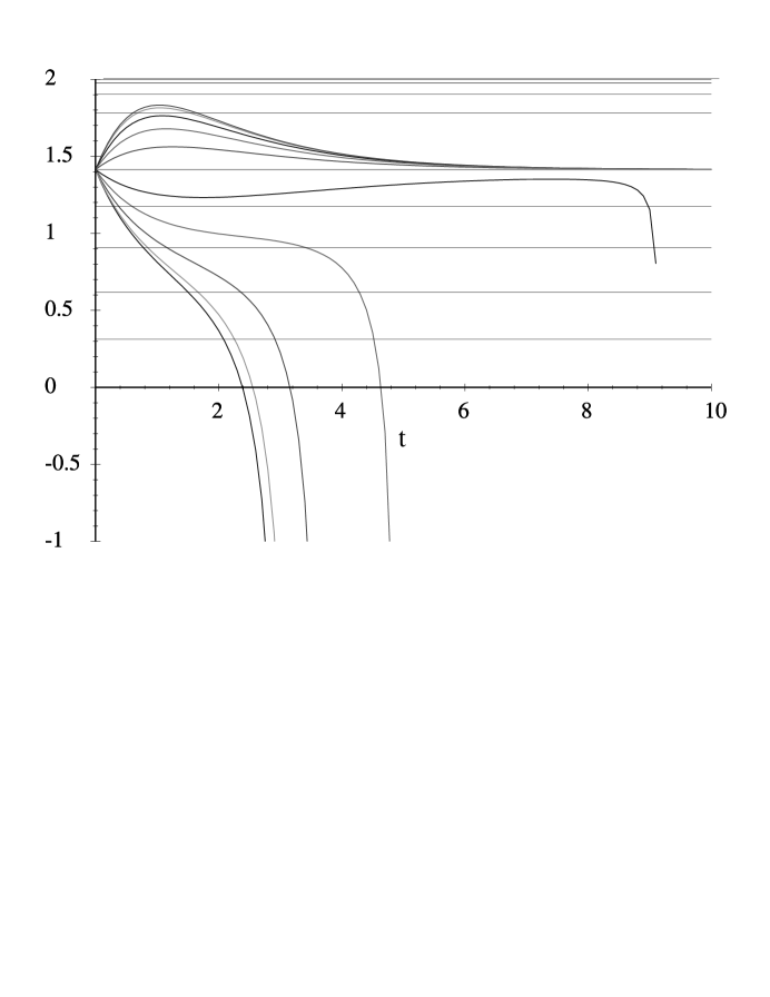
FIG. 6.: The scalar field theory frequencies $\gamma_{n}(k,t)$ obtained using an approximate contractor $T_{n}(t)$ for $n=1$ and various momenta $k$. The starting state is a product of uncorrelated Gaussians. The curves correspond to different values of $k$; the corresponding frequencies in the exact wavefunction are indicated by the horizontal lines.

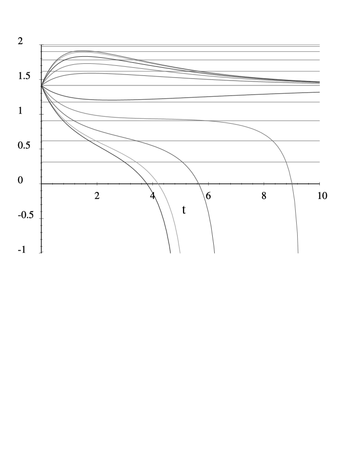
FIG. 7.: The frequencies $\gamma_{n}(k,t)$ as in Fig. 6, except that $n=2$.

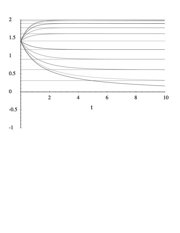
FIG. 8.: The frequencies $\gamma_{n}(k,t)$ as in Fig. 6, except that $n=40$.

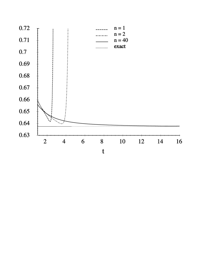
FIG. 9.: Expectation value of the free scalar field theory Hamiltonian in the state $T_{n}(t)\,|\Psi_{0}\rangle$ for $n=1,2$, and $40$, showing how the best $t$ changes as a function of $n$.

TABLE I.: Convergence of the partial sums $\epsilon_{n}$ in the cluster expansion of the free massless scalar-field vacuum energy density as a function of the range $n$. The energies are CORE estimates from a single-state per site truncation algorithm, and the errors are the differences of these estimates from the exact energy density 0.636619772.

$n$	$\epsilon_{n}$	Error
1	0.707107	0.070487
2	0.658919	0.022299
3	0.647644	0.011025
4	0.643206	0.006586
5	0.641001	0.004382
6	0.639746	0.003126
7	0.638962	0.002343
8	0.638441	0.001821
9	0.638076	0.001456
10	0.637811	0.001191
20	0.636932	0.000312
30	0.636761	0.000141
40	0.636700	0.000080

TABLE II.: Comparison of some of the couplings $\alpha_{s}^{(r)}$ in the renormalized Hamiltonian of a free scalar field theory for $r=2,3,4,\infty$, where $r$ is the cluster-expansion truncation order. Note that only $\alpha_{0}$ and $\alpha_{1}$ are defined for the case $r=2$.

$\alpha_{s}^{(r)}$	$r=2$	$r=3$	$r=4$	$r=\infty$
$\alpha_{0}$	$0.381966$	$0.371054$	$0.367594$	$0.363380$
$\alpha_{1}$	$-0.500000$	$-0.451922$	$-0.438360$	$-0.424413$
$\alpha_{2}$		$0.104212$	$0.098137$	$0.084883$
$\alpha_{3}$			$-0.041400$	$-0.036378$

TABLE III.: Comparison of truncated-cluster ${\cal E}_{r}$ and finite-volume $E_{r}/r$ Heisenberg antiferromagnet ground-state energy densities for range $r$.

$r$	${\cal E}_{r}$	$E_{r}/r$
2	$-0.3750000$	$-0.3750000$
4	$-0.4330125$	$-0.4040063$
6	$-0.4387760$	$-0.4155962$
8	$-0.4406775$	$-0.4218665$

REFERENCES

- [1] Colin J. Morningstar and Marvin Weinstein, Phys. Rev. Lett. 73, 1873 (1994).
- [2] For reviews, see K. G. Wilson, Rev. Mod. Phys. 47, 773 (1975); L. P. Kadanoff, in Phase Transitions and Critical Phenomena, edited by C. Domb and M. S. Green (Academic Press, London, 1974), Vol. 5a, p. 1); and K. Wilson and J. Kogut, Phys. Rep. C12, 75 (1974).
- [3] S. Drell, M. Weinstein, and S. Yankielowicz, Phys. Rev. D 16, 1769 (1977); R. Jullien, J. N. Fields, and S. Doniach, Phys. Rev. B 16, 4889 (1977) and Phys. Rev. Lett. 38, 1500 (1977); S. D. Drell, B. Svetitsky, and M. Weinstein, Phys. Rev. D 17, 523 (1978); S. D. Drell and M. Weinstein, ibid. 17, 3203 (1978); D. Horn and S. Yankielowicz, Nucl. Phys. B161, 533 (1979); K. Uzelac, P. Pfeuty, and R. Jullien, Phys. Rev. Lett. 43, 805 (1979); J. B. Bronzan and R. L. Sugar, Phys. Rev. D 21, 1564 (1980); D. Horn, M. Karliner, and S. Yankielowicz, ibid. B170, 467 (1980); D. Horn and M. Weinstein, Phys. Rev. D 25, 3331 (1982); H. R. Quinn and M. Weinstein, Phys. Rev. D 25, 1661 (1982); S. Ben-Menahem, ibid. 26, 455 (1982); J. Abad, J. G. Esteve, and A. F. Pacheco, ibid. 32, 2729 (1985); D. Horn, W. Langeveld, H. Quinn, and M. Weinstein, Phys. Rev. D38, 3238 (1988); G. Lana, ibid. 38, 1954 (1988); S. R. White and R. M. Noack, Phys. Rev. Lett. 68, 3487 (1992); S. R. White, ibid. 69, 2863 (1992); S. R. White, Phys. Rev. B 48, 10345 (1993).
- [4] J. Rabin, Phys. Rev. B21, 2027 (1980).
- [5] D. Horn and M. Weinstein, Phys. Rev. D30, 1256 (1984).
- [6] P. W. Anderson, Phys. Rev. 88, 694 (1952).
- [7] K. Wilson and M. E. Fisher, Phys. Rev. Lett. 28, 240 (1970).
- [8] N. Isgur and M. Wise, Phys. Lett. B232, 113 (1989); 237, 527 (1990); H. Georgi, Phys. Lett. B240, 447 (1990); E. Eichten and B. Hill, Phys. Lett. B234, 511 (1990); B243, 427 (1990).
- [9] B. A. Thacker and G. P. Lepage, Phys. Rev. D 43, 196 (1991).
- [10] S. K. Ma, Phys. Rev. Lett. 37, 461 (1976); R. H. Swendsen, Phys. Rev. Lett. 42, 859 (1979).
- [11] C. Domb, Adv. Phys. 9, 149 (1960).
- [12] G. S. Rushbrooke, J. Math. Phys. 5, 1106 (1964).
- [13] M. F. Sykes, J. W. Essam, B. R. Heap, and B. J. Hiley, J. Math. Phys. 7, 1557 (1966).
- [14] C. Domb in Phase Transitions and Critical Phenomena, edited by C. Domb and M. S. Green (Academic Press, London, 1974), Vol. 3, p. 1.
- [15] See, for example, David S. Watkins, Fundamentals of Matrix Computations (Wiley & Sons, New York, 1991) and J. W. Robbin, Matrix Algebra using MINImal MATlab (A. K. Peters, Ltd., Wellesley, MA, 1995).
- [16] N. D. Mermin and H. Wagner, Phys. Rev. Lett. 17, 1133 (1966).
- [17] H. A. Bethe, Z. Phys. 71, 205 (1931).
- [18] The t-J model was introduced in P. W. Anderson, Science 235, 1196 (1987). For a recent review, see E. Dagotto, Rev. Mod. Phys. 66, 763 (1994).
- [19] The Hubbard model was introduced in J. Hubbard, Proc. Roy. Soc. London, Ser. A 276, 238 (1963); extended Hubbard models contain additional interactions, most of which were considered but ultimately neglected in Hubbard’s original paper. For a review, see R. Micnas, J. Ranninger, S. Robaszkiewicz, Rev. Mod. Phys. 62, 113 (1990).
- [20] H. R. Quinn and M. Weinstein, Phys. Rev. D34, 2440 (1986).
- [21] K. G. Wilson in New Phenomena in Subnuclear Physics, (Erice 1975), edited by A. Zichichi (Plenum, New York, 1975).
- [22] H. R. Quinn, M. Weinstein, Phys. Rev. Lett. 57, 2617 (1986).
- [23] B. Svetitsky, S. D. Drell, H. R. Quinn, M. Weinstein, Phys. Rev. D22, 490 (1980).
- [24] M. Weinstein, S. D. Drell, H. R. Quinn, B. Svetitsky, Phys. Rev. D22, 1190 (1980).