KEK-CP-039

2D Quantum Gravity

-Three States of Surfaces-

A.Fujitsu , N.Tsuda and T.Yukawa

^† Information Systems and Technology Center The University of Aizu
Tsuruga, Ikki-machi, Aizu-Wakamatsu City Fukushima, 965-80, Japan

^‡ National Laboratory for High Energy Physics (KEK)
Tsukuba, Ibaraki 305, Japan

^§ Coordination Center for Research and Education,
The Graduate University for Advanced Studies,
Hayama-cho, Miura-gun, Kanagawa 240-01, Japan
and
National Laboratory for High Energy Physics (KEK)
Tsukuba, Ibaraki 305, Japan

Two-dimensional random surfaces are studied numerically by the dynamical triangulation method. In order to generate various kinds of random surfaces, two higher derivative terms are added to the action. The phases of surfaces in the two-dimensional parameter space are classified into three states: flat, crumpled surface, and branched polymer. In addition, there exists a special point (pure gravity) corresponding to the universal fractal surface. A new probe to detect branched polymers is proposed, which makes use of the minbu(minimum neck baby universe) analysis. This method can clearly distinguish the branched polymer phase from another according to the sizes and arrangements of baby universes. The size distribution of baby universes changes drastically at the transition point between the branched polymer and other kind of surface. The phases of surfaces coupled with multi-Ising spins are studied in a similar manner.

1 Introduction

Studies on two-dimensional surfaces are currently drawing much attention in various fields of science, such as physics, chemistry and biology. In physics, for example, the statistical property of triangulated surfaces is under intensive investigations in the context of two-dimensional quantum gravity. For a surface without coupled matter (pure gravity), a Monte-Carlo simulation by a dynamical triangulation(DT) method shows the fractal property, as predicted by such analytical theories as the Liouville field theory [1, 2, 3], the matrix model[4] and string field theory [5]. When matter, such as scalar fields, Ising spins or Potts models, is put on a surface it is expected that the surface becomes unstable toward forming a one-dimensional structure, like a branched polymer [6, 7]. We are interested in generating and classifying various kinds of surfaces. It is easy to imagine that there exist at least three kinds of surfaces, ( flat, crumpled surface and branched polymer), and wonder whether any surface can be classified into one of these three types. We would also like to investigate the nature of the transition between them. Furthermore, if the fluctuation of a surface can be visualized, it will be very useful for understanding the properties of surfaces and mutual transitions.

One of the important quantities which characterize a surface generated by the dynamical triangulation method is the discretized local scalar curvature;

$$R_{i}=\frac{2\pi}{a^{2}}\frac{(6-q_{i})}{q_{i}},$$ (1)

where $q_{i}$ (a coordination number) is the number of triangles sharing the vertex $i$, and $a^{2}$ is the area of an elementary triangle. As is well-known, the surface of pure gravity fluctuates strongly, containing many branches and spikes. A large positive curvature is localized at each tip of the spikes, and negative curvatures are condensed around the roots of the branches. Two additional terms are included in the action in order to control the local fluctuation of the surfaces. One is $\beta\int\sqrt{g}R^{2}d^{2}x$; the other is $\alpha\int\sqrt{g}g^{\mu\nu}\partial_{\mu}R\partial_{\nu}Rd^{2}x$ in continuous space, where $\alpha$ and $\beta$ are coupling constants. The former affects on the local curvature of surfaces;i.e. for a large positive $\beta$ it suppresses large fluctuations of $R$[8], and as $\beta$ becomes negative the surfaces become crumpled or branched polymers, depending on the sign of $\alpha$.

Since the smallest neck size of a branch is limited by the lattice constant, it is significant to consider the minimum necks. Only for the minimum neck can we locate its position uniquely. By measuring the area distributions and connectivities of each baby universe separated by the minimum necks we can distinguish branched polymers from other kinds of surfaces.

This paper is organized as follows: In the next section we briefly describe how the DT method is performed with two higher derivative terms in the action. In Section 3 we give a short review of the method of minimum neck baby universes (or ’minbu’[9]). In Section 4 we propose three phases to classify random surfaces, and discuss the properties of each phase. In Section 5 the transition between a crumpled surface (or a fractal surface) and a branched polymer is discussed, together with numerical simulation of random surfaces coupled with multi-Ising spins. In the last section we give a summary of our numerical results and a discussion.

2 Dynamical Triangulation with Higher
Derivative Terms

A study of two-dimensional quantum gravity offers not only a simple model of Einstein gravity, but also a general framework for providing the universal property of two-dimensional surfaces. Here, we employ the dynamical triangulation method [10] (DT), which is known to give the correct answer, expected from analytic theories.

In DT, calculations of the partition function are performed by replacing the path integral over the metric to the sum over possible triangulations of the two-dimensional surfaces by equilateral triangles. From the triangulation condition and the topological-invariance the total number of i-simplices ($N_{i}$) is related as

$$3N_{2}=2N_{1},$$ (2)

$$N_{2}-N_{1}+N_{0}=\chi,$$ (3)

where $\chi$ is the Euler number.

In practice we proceed with DT for a surface with an arbitrary genus as follows:

1. Initialization.

   Prepare equilateral 3-simplices(tetrahedrons), and put them together by gluing triangles face-to-face, forming a closed surface with a target genus. Then repeat the barycentric subdivision by choosing a triangle randomly until the area of the universe is reaches to the target size. This manipulation is equivalent to the so-called $(1,3)$ move.

2. Thermalization of configurations.

   For changing the geometry so as to bring the surface into thermal equilibrium, pick up a pare of neighbouring triangles randomly and flip the link shared by them(that is the flip-flop or $(2,2)$ move). This move conserves the area and topology of the surface, and is known to be ergodic, i.e. any two configurations of a fixed area and topology are connected by the finite sequence of the $(2,2)$ moves. The manifold conditions are always checked by requiring that any set of 2-simplexes having a 0-simplex in common should constitute a combinatorial 1-ball$(S^{1})$. We also restrict the geometry so as to not allow singular triangulations, such as self-energies and tadpoles, in the dual graph.

For the case of pure gravity the action is independent of the geometry, and all graphs generated by the flip-flop moves are accepted with equal weight as those of a canonical ensemble. In this case no dimensional parameter enters, and the surface is expected to be $fractal$.

Here, we introduce two additional terms in the action in order to produce various types of surfaces. There is a correspondence between a continuous theory(characterized by the metric tensor $g_{\mu\nu}$) and a discretized theory(characterized by the coordination number $q_{i}$) through a relation

$$\int\sqrt{g}d^{2}x\cdots\Longleftrightarrow\frac{a^{2}}{3}\sum_{i=1}^{N_{0}}q_{i}\cdots.$$ (4)

Two new terms are expressed in the language of discretized theory by making use of eqs.(1) and (4) as

$$\left\langle\int\sqrt{g}R^{2}d^{2}x\right\rangle\cong\frac{a^{2}}{3}\left\langle\sum_{i}q_{i}R_{i}^{2}\right\rangle=\frac{4\pi^{2}}{3a^{2}}\left\langle\sum_{i}\frac{(6-q_{i})^{2}}{q_{i}}\right\rangle$$ (5)

and

$$\left\langle\int\sqrt{g}g^{\mu\nu}\partial_{\mu}R\partial_{\nu}Rd^{2}x\right\rangle \cong \frac{1}{\sqrt{3}}\left\langle\sum_{<i,j>}(R_{i}-R_{j})^{2}\right\rangle$$ (6)

$$= \frac{1}{\sqrt{3}}\left\langle 2\sum_{i}q_{i}R_{i}^{2}-\frac{8\pi^{2}}{a^{4}}\sum_{<i,j>}(6-q_{i})(6-q_{j})/q_{i}q_{j}\right\rangle,$$

where $\langle\cdots\rangle$ means the ensemble average and $\langle i,j\rangle$ indicates a nearest-neighbour pair of vertices.

These two terms control the order of the vertices. The former favors a flat surface $({\it i.e.}\;\;q_{i}=6)$, and the latter creates a correlation of curvatures between neighbouring pairs of vertices producing such as crumpled surfaces or branched polymers for positive or negative parameter $\alpha$, respectively.

From eq.(6), since the $\int\sqrt{g}g^{\mu\nu}\partial_{\mu}R\partial_{\nu}R$ term contains the $R^{2}$ term, we thus rearrange it into the $\sum_{<i,j>}(6-q_{i})(6-q_{j})/q_{i}q_{j}$ term in numerical simulations instead of the r.h.s. of eq.(6). Then, the Lattice action is

$$S=\beta_{Lattice}\sum_{i}\frac{(6-q_{i})^{2}}{q_{i}}+\alpha_{Lattice}\sum_{<i,j>}\frac{(6-q_{i})(6-q_{j})}{q_{i}q_{j}},$$ (7)

where the script $Lattice$ indicates a dimensionless coupling,

$$\left\{\begin{array}[]{ll}\displaystyle{\alpha=-\frac{\sqrt{3}a^{4}}{8\pi^{2}}\alpha_{Lattice}},\\[14.22636pt] \displaystyle{\beta=\frac{3a^{2}}{4\pi^{2}}(\alpha_{Lattice}+\frac{1}{36}\beta_{Lattice})}.\end{array}\right.$$ (8)

Since these two higher derivative terms (eqs.(5) and (6)) have dimensions of $a^{-2}$ and $a^{-4}$, respectively, they are irrelevant in the continuum limit. The typical short-distance scale introduced by the $R^{2}$ term is $\sim\sqrt{\beta}$, within which the surfaces are controlled to be smooth, and we need to set $\beta>A$ in order to maintain an effect on surface significant over area $A$.

When both terms are included, it may be possible to construct an effective theory coupled with a scalar field by introducing an auxiliary field ($\chi$) and defining a theory for the case $\beta>0$ by the action

$$\int d^{2}\xi\sqrt{g}(\frac{-\alpha}{\beta^{2}}g^{\mu\nu}\partial_{\mu}\chi\partial_{\nu}\chi+\frac{1}{\beta}\chi^{2}-i\chi R),$$ (9)

and for $\beta<0$,

$$\int d^{2}\xi\sqrt{g}(\frac{-\alpha}{\beta^{2}}g^{\mu\nu}\partial_{\mu}\chi\partial_{\nu}\chi+\frac{1}{\beta}\chi^{2}+\chi R).$$ (10)

We then integrate out the auxiliary field formally, giving

$$\int d^{2}\xi\sqrt{g}R\frac{1}{\frac{1}{\beta}+\frac{\alpha}{\beta^{2}}\Delta}R,$$ (11)

obtaining the effective action,

$$S=\int\sqrt{g}d^{2}\xi(\alpha g^{\mu\nu}\partial_{\mu}R\partial_{\nu}R+\beta R^{2}),\;\;\;\;\;\;\mbox{for}\;|\alpha|\ll|\beta|,$$ (12)

in a perturbative expansion using the parameters $\frac{\alpha}{\beta}$. In order to guarantee the perturbative expansion of eq.(11), $\alpha$ and $\beta$ must be restricted to $|\alpha|\ll|\beta|$ . It is important to notice that the ratio of the couplings, $\frac{\alpha}{\beta^{2}}$, can be fixed to be finite, while both parameters $\alpha$ and $\beta$ are taken to have infinite simultaneity in order to keep the effects significant in the continuum limit. Since the signs of the kinetic terms of eqs.(9) and (10) must be positive, it is required that $\alpha<0$. We again discuss the validity of the model of eq.(9) in subsection $4.1$.

3 Analysis of the baby universes

In order to discuss the stability (or instability) of two-dimensional surfaces, we consider the so-called minimum-neck baby universes, as were mentioned in section 1. A minimum-neck baby universe is defined as a connected sub part of a surface whose area must be less than half of the total area, and the neck is constructed by three links which are closed, non-self intersecting. A mother universe is defined as a minimum-neck universe whose area is greater than half the total area.

Suppose two kinds of surface configurations(in Fig.1(a)): one is a non-branched sphere, whose volume is $A$; the other is branched sphere which has a baby universe(volume $B$). Once the latter configuration is favorable, all universes branch out boundlessly. Then, a bottle neck becomes a minimum-length neck, which leads to lattice-branched polymers. Instabilities make the surfaces branched, and simultaneously the mother universe disappears. Whether there exists a mother universe or not is one of the differences between branched polymers and other kinds of surfaces.

It is easy to show that the relationship between of the string susceptibility to the branched polymer instability[11], for the partition function with the total area constrained to $A$ given by

$$Z(A)\sim\kappa^{A}A^{\gamma-3}.$$ (13)

For the case of a branched configuration (Fig.1(a)), we can estimate a lower bound for this contribution,

$$\int_{\frac{A}{3}}^{\frac{2A}{3}}dBZ(B)Z(A-B)B(A-B)\sim\kappa^{A}A^{2\gamma-3}.$$ (14)

Since Z[A] is the total number of distinct graphs with $A$ triangles and $S^{2}$ topology, $BZ[B]$ is the total number of distinct graphs with $B$ triangles and $D^{2}$ topology for a boundary loop length of 3.

The dominance of the branched polymer configuration corresponds to the case of $\gamma>0$. Thus, it is natural to recognize that a positive $\gamma$ corresponds to the case $c>1$. So far, since there have been no exactly solvable models with $c>1$, it is important to measure the actual minbu distributions for various kinds of DT surfaces in order to understand the dynamics of a 2d surface.

In practice, it is easy to identify all of the minimum necks, and their connectivities on real dynamically triangulated graphs without self-energies and tadpoles in a dual graph. The procedures are as follows:

• Pick up one link. There are then two vertices at both edges of this link; each vertex connects with many other links. Among them(links) a common vertex may be contained; unless these three links form a $2$-simplex (${\it i.e.}$ a triangle) we call these closed links a minimum neck. A smaller part of the two universes separated by this minimum neck is a minbu. Repeat this process until all of the links are checked. This is applicable to the configurations of a nest of baby universes.

• The connectivities of each baby universe are easily found. The key property is that a neck always separates universe into two parts for a spherical topology. First, pick up an arbitrary neck; then, two separated universes ($U1,U2$) can be identified. Second, choose a neck which belongs to universe $U1$(or $U2$); then, $U1$(or $U2$) can be decomposed into two sub parts: $U11,U12$(or $U21,U22$). Repeat until all of the necks have been checked. After this, it is straightforward to know the area distributions of all universes.

The minbu analysis can also visualize a triangulated surface as a network of baby universes connected by minimum necks (Fig.1(b)). In the next section we apply this analysis in order to classify the surfaces.

A measurement of the minbu distributions provides the string susceptibility ($\gamma_{s}$) with high accuracy[12]. The probability of finding a minbu with area $B$ in a universe having a total area of $A$ is given by

$$P_{A}(B)=\frac{3BZ[B](A-B)Z[A-B]}{Z[A]}$$ (15)

In order to obtain the frequency of finding a minbu ($N_{A}(B)$) with volume $B$ for the case of pure gravity, we substitute the KPZ formula into eq.(15), giving

$$N_{A}(B)\sim A^{\gamma_{s}-1}\left(\frac{B}{A}\right)^{\gamma_{s}-2}\left\{1-\left(\frac{B}{A}\right)\right\}^{\gamma_{s}-2},$$ (16)

where $\gamma_{s}=-\frac{1}{2}$.

It is easy to extract the $\gamma_{s}$ from numerical data when the KPZ formula is applicable. It should be remarked that in the case of $c\neq 0$ the finite size corrections for eq.(16) become important. Even in the case of one Ising spin coupled to gravity (correspond to $c=\frac{1}{2}$), the finite size corrections are not negligible, and without a proper correction it is not possible to define the correct $\gamma_{s}(=\frac{1}{3})$ with the same accuracy as in the case of $c=0$ [13].

Figure 1: $(a)$ Non branched surface with volume A and a branched surface which includes one baby universe with volume B. $(b)$ A surface generated by the DT method visualized as a network of baby universes. One of the examples of the transition between fractal(or crumpled) surfaces to branched polymers is also visualized.

4 Phase Diagram

Let us classify typical states of surfaces generated by the two additional higher derivative terms in the action. We would like to propose that any surfaces are constituted by a branched polymer, a crumpled surface and a flat one. We can intuitively explain how these kinds of surfaces are created. The term $\sum_{i}(6-q_{i})^{2}$ with a positive coefficient favors $q_{i}=6$, $i.e.$ a flat surface. On the other hands, the term $\sum_{i}(6-q_{i})^{2}$ with a negative coefficient favors crumple surfaces rather than branched polymers. The term $\sum_{<i,j>}\frac{(6-q_{i})(6-q_{j})}{q_{i}q_{j}}$ with a positive coefficient also makes surfaces crumple, because the opposite-sign curvatures of adjacent vertices become attractive. On the contrary the term $\sum_{<i,j>}\frac{(6-q_{i})(6-q_{j})}{q_{i}q_{j}}$ with a negative coefficient makes surface branched polymers, because same-sign curvatures are attractive. For the root(the loop of negative curvatures) and tip(a hemisphere of positive curvatures), those curvatures having the same sign need to condense to form a branched polymer.

In order to classify the surface, we have observed $Q_{2}$ and $Q_{3}$ which are ensemble-averaged quantities ($cf$ eqs.(5) and (6)), defined on the lattice as follows:

$$Q_{2}\equiv\langle\sum_{i}\frac{(6-q_{i})^{2}}{q_{i}}\rangle/N_{2},$$ (17)

$$Q_{3}\equiv\langle\sum_{<i,j>}\frac{(6-q_{i})(6-q_{j})}{q_{i}q_{j}}\rangle/N_{2}.$$ (18)

Figs.2 and 3 clearly show that there are three plateaus, which indicate that the DT surfaces can be classified into three characteristic states ($i.e.$ crumpled, flat and branched polymer) depending on the two parameters which we have employed.

Figure 2: Plot of $Q_{2}$ versus $\alpha$ and $\beta$.

Figure 3: Plot of $Q_{3}$ versus $\alpha$ and $\beta$.

We have also measured the size-distribution and arrangements of all minimum-neck baby universes on these three plateaus. The features of these three surfaces are itemized as follows:

1. Crumpled Surface ($\alpha>0,\beta<\alpha$) :

   This surface looks jagged. The value of $Q_{2}$ becomes much larger than in the flat case, and that of $Q_{3}$ becomes negative. A mother universe exists whose volume reaches the order of $60\%$ or $70\%$ of the total area, although the growth of large branches is highly suppressed(see Fig.5). All baby universes have a small volume ($\sim{\cal O}(1)$). The number of minimum necks is about $8\sim 9\%$ of the total number of triangles.

2. Flat Surface ($\beta>|\alpha|$) :

   Almost all fluctuations are suppressed ($i.e.$ $Q_{2}\approx Q_{3}\approx 0$), and the fractal dimension becomes about $2.0$.

3. Branched Polymer ($\alpha<0,\beta<|\alpha|$) :

   One of the typical branched polymers is illustrated by the r.h.s. of Fig.1$(b)$. The mother universe completely disappears. All baby universes are very small ($\sim{\cal O}(1)$). The number of minimum necks is about $30\sim 40\%$ of the total number of triangles.

At the $N_{2}\to\infty$ limit of the branched polymer its surface can no longer be regarded as being a smooth continuum medium. In order to check this, we measured the resistivities (correspond to the complex structures defined on DT surfaces) of branched polymers based on ref.[7]. If there exists a smooth continuum limit of this surface, the peaks of resistivity become narrower as the size increases. Fig.4 is a plot of a normalized histogram of the resistivities for branched polymers. As has been expected above, Fig.4 shows that there is no sharpening of the peaks as the size increases. That indicates that a branched polymer has no continuum limit.

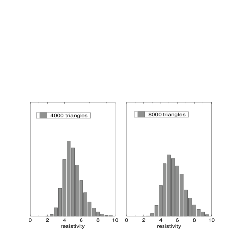
Figure 4: Normalized histogram of the resistivities[7] for the case of branched-like surfaces: $\alpha=-10,\beta=0$.

Furthermore we point out the characteristic property based on an intrinsic geometrical point of view of these three states, that is, the distributions of the number of boundaries (branches) versus the geodesic distances ($D$). A definition of the boundaries (branches) is given in the next subsection ($4.2$). Fig.5 supports the intuitive pictures that we mentioned above. Especially, the dashed-dotted line (correspond to the crumpled space-time) indicates that the large branch structures are highly suppressed. This tendency coincides with that of a case of three-dimensional simplicial gravity[14].

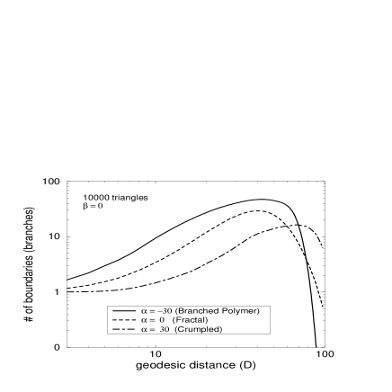
Figure 5: Distributions of the number of boundaries (branches) versus the geodesic distance for various states with double-log scales. The solid line represents branched polymer states, the dotted line represents the case of pure gravity (fractal states) and the dashed-dotted line represents crumpled states.

4.1 Flat states ($R^{2}$-gravity)

Here, we consider in detail the almost flat states of DT surfaces. At first, we investigate the minbu distributions for a large positive $\beta$ ($\alpha$ = 0) [15]. In ref.[8] the partition function and the string susceptibility have been estimated to be the following asymptotic form for $\frac{A}{\beta}\to 0$ and $A\to\infty$:

$$Z^{KN}\sim A^{\gamma^{KN}_{s}-3}\exp(-64\pi^{2}(1-h)^{2}\cdot\frac{\beta}{A})e^{-\mu A},$$ (19)

where

$$\gamma^{KN}_{s}(\chi,\frac{A}{\beta})=2+\frac{d-12}{12}\chi+\frac{d}{768\pi^{2}}\frac{A}{\beta}.$$ (20)

Here, $\chi$ is the Euler number of this surface, and $d$ is the central charge of the matter fields. For the case of $d=0$ and $\chi=2(\mbox{sphere}:S^{2})$, $\gamma^{KN}_{s}$ becomes zero. In Fig.6 we plot and compare the minbu distributions ($N_{A}(B)$) versus $B(1-\frac{B}{A})$ with the double-log scale for $\beta_{Lattice}=100$ and $200$ with a total number of triangles 5000. Since the $R^{2}$ term affects only on the short-distance property of surfaces, it is expected that eq.(20) is adaptable for a relatively small minbu region. Fig.6 shows a good agreement with numerical data(open circle and square), and an asymptotic formula (dashed-line) which is obtained by substituting eq.(19) into eq.(15) within the small $B$ regions . We note that the data points approach the line predicted for the pure-gravity case ($\gamma_{s}=-\frac{1}{2}$) in large minbu regions. This indicates that the $R^{2}$ term is irrelevant with respect to long-range structures.

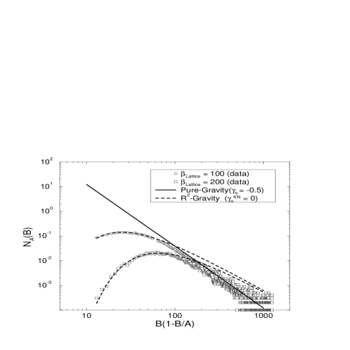
Figure 6: Minbu area distributions ($N_{A}(B)$) for $R^{2}-$gravity with topology $S^{2}$ with the double-log scales. The total number of triangles is 5,000. $B$ represents the area of a baby universe. The solid line represents the minbu area distributions for the pure-gravity case (eq.(16)). The two dashed lines show the fit curve predicted by $R^{2}-$gravity [8] with $\beta_{Lattice}$ = 100 and 200.

When we consider a part of a flat parameter region, $0<\alpha_{Lattice}\ll\beta_{Lattice}$, the model of eq.(9) corresponds to our numerical simulations. The string susceptibility ($\gamma^{KN}_{s}$) of the model (9) was also obtained by ref.[8] in the asymptotic form for $\frac{A}{\beta}\to 0$ and $A\to\infty$,

$$\gamma^{KN}_{s}=2-\left(\frac{24+\eta}{12}+\frac{1}{32\pi}\cdot\frac{\beta^{2}}{\alpha}\sqrt{\frac{24+\eta}{\eta}}\right)\frac{\chi}{\alpha_{-}}-\frac{d}{8\pi\alpha_{-}\eta}\cdot\frac{\beta^{2}}{\alpha}\sqrt{\frac{24+\eta}{\eta}}\cdot\frac{A}{\beta},$$ (22)

where $\eta\equiv-\frac{3}{8\pi}\cdot\frac{\beta^{2}}{\alpha}-d$ and $\alpha_{-}\equiv\frac{1}{12}(24+\eta-\sqrt{\eta(24+\eta)})$. It is remarkable that the $\gamma^{KN}_{s}$ of eq.(22) does not depend upon $\alpha$, and is the same as $\gamma_{s}$ of eq.(20) when $d=0$. The plateau(corresponds to $|\alpha|<\beta$) observed in Figs.2 and 3 indicates the $\alpha$-independence of $\gamma^{KN}_{s}$.

As reported in ref.[16, 17], the transition from the fractal configuration to the flat configuration was a cross-over. It can be realized by varying $\beta$ with $\alpha=0$ in our case. In Fig.7 we plot $Log(Q_{2})$ versus $Log(\beta_{Lattice})$, comparing the semiclassical calculation (see appendix A) and numerical results with the total number of triangles ($20,000$). A semi-classical analysis shows the excellent agreement with the numerical data at $\beta\approx 0$ and large $\beta$.

Figure 7: Plot of $Log_{10}(Q_{2})$ versus $Log_{10}(\beta_{Lattice})$, comparing the semi-classical calculation and numerical results with a total number of triangles of $20,000$. The filled circles represent the numerical data with $\alpha_{Lattice}=0$ and $\beta_{Lattice}=0.01\sim 300$; the thin line is a guide. The thick line represents a semi-classical analysis. (See Appendix A).

4.2 Fractal structures at $\alpha\sim\beta\sim 0$

The most significant transition point is at ($\alpha\sim\beta\sim 0$). Here, no scale parameters exist, and the surfaces are expected to become a fractal. We now define the intrinsic geometry using the concept of a geodesic distance between two triangles on a DT surface. Suppose that a disk which is covered within $D$ steps from some reference triangle. Because of the branching of the surface, a disc is not always simply-connected, and there usually appear many boundaries which consist of $S^{1}$ loops in this disc. In order to show the fractal properties of the DT surface, the loop-length distribution function ($\rho(L,D)$) is measured by counting the number of boundary loops with the length $L$ which make boundaries of the area covered within $D$ steps. In ref.[4] it has been predicted that the loop-length distribution is a function of the scaling variable, $x=l/d^{2}$, in the continuum limit for pure gravity, where $l$ is the loop length and $d$ is a distance defined on the continuum surfaces. For simplicity we do not distinguish continuous variables ($l,d$) from lattice variables ($L,D$). In Fig.8 the results of our simulation for various distances are compared to the theory for a surface with the size of $20,000$ triangles. The distributions with different distances show an excellent agreement with each other and the shapes of the numerical data and the theoretical curve are quite similar. At the same time, artifacts of a lattice at small $x$ and the finite-size effects at large $x$ are observed. We have also investigated for several sizes of surfaces, $i.e.$ $100,000$ and $400,000$ triangles [16], and the same quantities have been given(but low statistics). These excellent agreements with the numerical results and the analytical approach make it clear that the DT surface becomes fractal in the sense that sections of the surface at different distances from a given point look exactly the same after a proper rescaling of the loop lengths. The loop-length distribution function comprises two types of loops corresponding to the exponent: baby loops and a mother loop. The baby loops dominate the loop length, and give the fractal dimension $4$; however, their averaged length is on the order of the cut-off length, and they are non-universal, and it cannot be considered as the proper fractal dimension of this surface. There always exists one mother loop with length proportional to $D^{2}$, which has a fractal dimension of 3. In our earlier simulations[18], we found that the naive fractal dimension reached about $3.5$ with $400,000$ triangles.

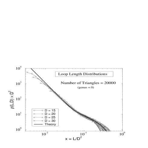
Figure 8: Loop-length distributions with the double-log scales. The total number of triangles is 20,000, and is averaged over 1000 configurations. $x={L}/{D^{2}}$ is a scaling variable, where $D$ represents the geodesic distance (it was measured at steps $D=15,20,25,30$) and $L$ represents each loop length at step $D$. The small circles, quadrangles and triangles indicate the results of numerical simulations; the solid line indicates the theoretical curve predicted by string field theory[4].

5 Transition to a Branched Polymer

The $\alpha$ term ($\alpha>0$) favors the attraction of vertices with the opposite-sign curvature. If this coefficient still becomes larger, this effect exceeds the $R^{2}$ term effect, and the surface crumples. On the other hand, a negative coefficient ($\alpha<0$) makes a transition to the branched polymer. In Fig.1$(b)$ we illustrate one such kind of transition.

The important point to note is the volume distributions of a mother universe and a baby one. For fractal surfaces(corresponding to the pure-gravity case), a mother universe has a large volume $i.e.$ $\sim$ half of the total volume( ${\cal O}(N_{2})$), and the sizes of the other baby universes are very small (${\cal O}(1)$). On the other hand, for branched polymer configurations all of the baby universes have small sizes and no mother universe exists. We therefore propose a new order parameter($RV_{1,2}$) for the transition to the branched polymer,

$$RV_{1}\equiv\frac{V_{max}}{V_{total}}\;\;\mbox{or}\;\;RV_{2}\equiv\frac{V_{second}}{V_{max}},$$ (23)

where $V_{max}$ represents the maximum area among all of the universes in this surface, and $V_{second}$ represents a secondary size universe. Indeed, we examined that $RV_{1,2}$ works well as an indicator of such kinds of transitions in numerical simulations. Fig.9 shows the $RV_{2}$ versus $\alpha_{Lattice}$ with the range: $[-50,50]$. A clear transition can be seen from the branched polymer to crumpled or fractal surfaces.

In Figs.10 and 11 we also show $RV_{1}$, as well as the total number of minimum necks versus $\alpha_{Lattice}$, respectively. These data (Fig.9,10 and 11) suggest that the DT surfaces become a branched polymer for $\alpha<-10$. As has been mentioned, our numerical systems correspond to the effective theory coupled with a scalar field; also $\alpha$ must be negative ($i.e.$ $\alpha_{Lattice}$ must be positive). Then, the branched polymer stands for the appearance of some instabilities of the system. In our results if $\alpha_{Lattice}<0$ means the negative coefficient of the kinetic term (9), and the stability of the surfaces certainly disappear.

Figure 9: $RV_{2}$ plotted versus $\alpha_{Lattice}$. The total number of triangles is 2,000, and $\beta=0$. The statistical errors were estimated to be about $10$%.

Figure 10: $RV_{1}$ plotted versus $\alpha_{Lattice}$. The other conditions are the same as in Fig.9.

Figure 11: Total number of minimum necks plotted versus $\alpha_{Lattice}$. The numerical data are indicated by filled circles. The other conditions are the same as in Fig.9.

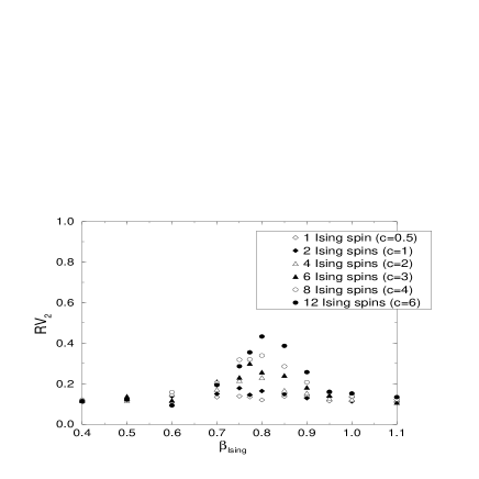
Figure 12: $RV_{2}$ plotted versus the coupling constant of the Ising spins ($\beta_{Ising}$). The open diamond indicates one Ising spin($c=0.5$), the close diamond indicates two Ising spins($c=1$), the open triangle indicates 4-Ising spins($c=2$), the close triangle indicates 6-Ising spins($c=3$), the open circle indicates 8-Ising spins($c=4$) and the close circle indicates 12-Ising spins($c=6$). The total number of triangles is 2,000, and averaged by 500 ensembles for each data.

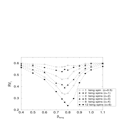
Figure 13: $RV_{1}$ ($V_{total}=2000$) plotted versus $\beta_{Ising}$; the other conditions are the same as in Fig.12.

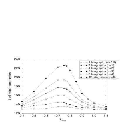
Figure 14: Total number of minimum necks plotted versus $\beta_{Ising}$; the other conditions are the same as in Fig.12.

5.1 Matter($c>1$) coupled with gravity

There are many theoretical indications that the surfaces degenerate into branched-polymer configurations for $c>1$. We investigated the case of multi-Ising spins coupled to gravity using the minbu analysis. Each Ising spin lives on a triangles, and is thermalized by using cluster updates[19]

It is rather difficult to obtain clear signals for such transitions when n-Ising spins are coupled to gravity. In Figs.12, 13 and 14 we plot $RV_{2,1}$ and the averaged total number of minimum necks of the surface as a function of the coupling strength of the Ising spins, respectively. All of these observables slowly change with the central charge; however, it is certain that the effect of matter makes the surfaces branched for a sufficiently large $c$.

It seems natural that the Ising spins living on a small-size baby universes, or branched polymers, suffer considerably from finite size effects. It is thus expected that such spins decouple with the background geometries. This is the main reason that the transition is not very clear.

6 Summary and Discussion

We have classified the two-dimensional random surfaces generated by dynamical triangulation into three states (crumpled surface, flat surface and branched polymer) varying the strength of two interaction terms. The three states are characterized by local observables, such as average square curvatures ($Q_{2}$) and the average square-curvature derivative ($Q_{3}$). The $R^{2}-$gravity in the strong coupling limit $\frac{\beta}{A}\to\infty$, gives the flat-surface, which was established numerically. We could also explain the cross-over phenomenon between the fractal and flat states within the perturbative colculations. Furthermore, we examined why the surfaces become crumple rather than a branched polymer in the region of $\alpha_{Lattice}>0,\beta_{Lattice}<\alpha_{Lattice}$. On the other hand we observed that the surface becomes branched polymers with $\alpha_{Lattice}<0,\beta_{Lattice}<|\alpha_{Lattice}|$, and that the measurements of its resistivities clarify that this surface does not have a smooth continuum limit. The minbu analysis showed the nested structure of random surfaces directly; it also gave one important clue for distinguishing branched polymers from other kinds of surfaces. As to whether a mother universe exists or not, we quantitatively propose an observable, $RV_{1}\equiv\frac{V_{max}}{V_{total}}$ or $RV_{2}\equiv\frac{V_{second}}{V_{max}}$. In fact, the $RV_{1,2}$ works well in our simulations. The good fractal structure which is known in the case of pure gravity ($\alpha\sim\beta\sim 0$) disappears in each of three states; on crumpled surfaces large branches can not grow enough, and on branched polymers a mother universe disappears, while branching into many small baby universes, which means a disappearance of the mother loop in the distribution of the loop length. We also applied the same analysis to the case of multi-Ising spins coupled to gravity corresponding to $c=1,2,4,6,8,12$. The $RV_{1,2}$ smoothly varies, and the number of minimum necks slowly grows with the central charges.

The kinetic terms of the auxiliary field of eqs.(9) and (10) have negative signs for $\alpha_{Lattice}<0$ within which we observed the branched polymer configurations in our numerical simulation. Since we do not know a connection between the effective theory coupled to a scalar field and the numerical simulation clearly, the central charge ($c$) which corresponds to the DT surfaces cannot be estimated precisely. However, we can be fairly certain that these branched polymers are related to the $c>1$ instabilities of the surfaces. We therefore need to inquire further into the intimate correspondences between the numerical simulations and continuum theory.

Acknowledgements

We would like to thank H.Hagura, H.Kawai, H.S.Egawa, J.Nishimura, N.Ishibashi and S.Ichinose for useful discussions and comments. One of the authors (N.T.) was supported by a Research Fellowship of the Japan Society for the Promotion of Science for Young Scientists.

Appendix

Appendix A Semi-classical calculation of $R^{2}$-gravity

In this appendix we consider a semiclassical treatment based on a ref. [20] of $R^{2}$-gravity in order to account for the cross-over transition between a flat surface and a fractal surface.

The partition function for surfaces with a fixed area of $A$ is defined by

$$Z[A]=\int{{\cal D}g_{{\mu\nu}}{\cal D}X\over\hbox{\it Vol.(Diffeo)}}{\hbox{e}}^{-S_{G}[g]-S_{m}[X]}\delta\left(\int dx^{2}\sqrt{g}-A\right),$$

where $S_{G}[g]=\int d^{2}x\sqrt{g}(\lambda+\beta R^{2}),$ and $S_{m}[X]$ is the matter action given by $S_{m}[X]=\int d^{2}x\sqrt{g}g^{\mu\nu}\partial_{\mu}X^{a}\partial_{\nu}X^{a},\quad a=1\sim d.$

Taking the conformal gauge $g_{{\mu\nu}}=\hat{g}_{{\mu\nu}}e^{\phi}$, and estimating the FP-determinant and the integral of matter fields, we have

$$Z(A)=\int{{\cal D}_{g}\phi\over\hbox{\it Vol.(C.G.)}}{\hbox{e}}^{-S_{G}[\hat{g}{\hbox{e}}^{\phi}]-{26-d\over 96\pi}\int d^{2}x\sqrt{g}(-\phi\Delta_{1}\phi+2R\phi)}\delta\left(\int d^{2}x\sqrt{\hat{g}}{\hbox{e}}^{\phi}-A\right),$$

where $\Delta_{1}$ is the Laplacian of $S^{2}$ with radius $1$. Then, integrating the constant mode of $\phi$, which is only used to estimate the $\delta$-function, as $\phi_{0}=\ln A-\ln{G[\tilde{\phi}]}$, where $G[\tilde{\phi}]=\int d^{2}x\sqrt{\hat{g}}{\hbox{e}}^{\tilde{\phi}}$, we obtain

$$Z(A,\beta)=A^{d-20\over 6}{\hbox{e}}^{-\lambda A}\int{\cal D}_{\hat{g}}\tilde{\phi}{\hbox{e}}^{-\tilde{S}[\tilde{\phi}]},$$

where the action for oscillating parts, $\tilde{\phi}=\phi-\phi_{0}$, is now

$$\tilde{S}[\tilde{\phi}]=\int d^{2}x\sqrt{g_{1}}\left({\beta G[\tilde{\phi}]\over Ar^{2}}(2-\Delta_{1}\tilde{\phi})^{2}{\hbox{e}}^{-\tilde{\phi}}-{1\over 2\gamma}\tilde{\phi}\Delta_{1}\tilde{\phi}-{2\over\gamma}\ln G[\tilde{\phi}]\right).$$

Here we have written $\gamma={48\pi\over 26-d}$. Now, we make a weak field expansion, and take only the quadratic terms with respect to the field, $\tilde{\phi}$. The functional integral is carried out by expanding $\phi$ in terms of spherical-harmonic functions. Finally, we obtain the expression

$$Z(A,\beta)=A^{d-20\over 6}{\hbox{e}}^{-\lambda A-{64\pi^{2}\beta\over A}}\prod_{l\geq 2}^{L}(\omega_{l})^{-{2l+1\over 2}},$$

where

$$\omega_{l}={(4\pi)^{2}\beta\over A^{2}}(l(l+1)-2)^{2}+{2\pi\over\gamma}{(l(l+1)-2)\over A}.$$

The zero-frequency modes with $l=1$ correspond to the conformal Killing modes, and have been omitted in the functional integral.

For a large $\beta$, the determinant part is

$$\matrix{\sum_{l\geq 2}^{L}(2l+1)\ln\omega_{l}\sim&\left(2L(L+2)-{8\over 3}+{A\over 8\pi\beta\gamma}\right)\ln L^{2}-2L^{2}\hfill\cr&-2(L(L+2)-3)\ln A+(L(L+2)-3)\ln(16\pi^{2}\beta).\hfill}$$

The ultra-violet cut-off of an angular momentum ($L$) will be fixed by $L(L+2)=A\Lambda^{2}$. We obtain

$$\sum_{l\geq 2}^{L}(2l+1)\ln\omega_{l}\sim\kappa_{0}+\kappa_{1}(\beta)A+\left({10\over 3}+{A\over 8\pi\beta\gamma}\right)\ln A-3\ln(16\pi^{2}\beta),$$

where $\kappa_{0}$ and $\kappa_{1}$ are divergent when the cut-off ($\Lambda$) goes to infinity.

For small $\beta$, we have

$$\sum_{l\geq 2}^{L}(2l+1)\ln\omega_{l}\sim\kappa_{0}^{\prime}+\kappa_{1}^{\prime}(\beta)A+{5\over 3}\ln A+3\ln\left({\gamma\over 2\pi}\right).$$

In order to compare the semi-classical calculation with the numerical results, we should make a correspondence of the cut-off ($\Lambda$) with $N_{2}$ as $L(L+2)=A\Lambda^{2}=\kappa N_{2}$, where $\kappa$ is a constant which should be determined based on the numerical data. Using the asymptotic formulas eqs.$(A.8)$ and $(A.9)$, we obtain $\langle\int d^{2}xR^{2}\rangle=-\frac{\partial\log Z}{\partial\beta}$ for large $\beta_{Lattice}$,

$$a^{2}\left\langle\int\sqrt{g}R^{2}d^{2}x\right\rangle=48\pi^{2}N_{2}\left\{\frac{\kappa}{2\beta_{Lattice}}+\frac{4}{3N^{2}_{2}}+\frac{6\pi\ln({\kappa N_{2}})}{\beta_{Lattice}^{2}\gamma}\right\},$$

and for small $\beta_{Lattice}$

$$a^{2}\left\langle\int\sqrt{g}R^{2}d^{2}x\right\rangle=12\pi N_{2}\gamma\left\{\frac{\kappa^{2}}{6}+\frac{1}{N_{2}}\right\}.$$

We are able to determine the value of $\kappa$ from a data point, for example $(Q_{2},\beta_{Lattice})$ = $(0.0449\pm 0.0005,200)$. From eqs.(5),(8),(17) and ($A.10$) we obtain

$$\kappa=0.499\pm 0.005,$$

which is consistent with ref.[16].

From eq.($A.6$) we can calculate $\langle\int d^{2}x\sqrt{g}$ $R^{2}$ $\rangle$ without using the asymptotic formulas given above. We thus have

$${\left\langle\int d\Omega R^{2}\right\rangle\over 48\pi^{2}N\Lambda^{2}}={4\over 3N^{2}}+{1\over N}\sum_{l\geq 2}^{\sqrt{\kappa N}}{2l+1\over 2}{{1\over N}(l(l+1)-2)\over{\beta_{Lattice}\over N}(l(l+1)-2)+{6\pi\over\gamma}},$$

which can well reproduce the data (Fig.7) in both ranges of small and large $\beta$, when we choose the parameter $\kappa$ to be 0.5.

The values of $\gamma_{string}$ given through semi-classical calculation,

$$\gamma_{string}=\left\{\matrix{{d-7\over 6}\hfill&\quad\hbox{ for small }\beta\cr{d-12\over 6}+{(d-26)A\over 768\pi^{2}\beta}\hfill&\quad\hbox{ for large }\beta,}\right.$$

is exact in a large (-$d$) limit. If one wants to obtain correct values for all $d$, a full quantum treatment is necessary.

References

- [1] V.G.Knizhnik, A.M.Polyakov and A.B.Zamolodchikov, Mod.Phys.Lett. A3 (1988) 819.
- [2] J.Distler and H.Kawai, Nucl.Phys. B321 (1989) 509.
- [3] F.David, Mod.Phys.Lett. A3 (1988) 1651.
- [4] H.Kawai, N.Kawamoto, T.Mogami and Y.Watabiki, Phys.Lett. B306 (1993) 19; N.Ishibashi and H.Kawai, Phys.Lett. B322 (1994) 67.
- [5] N.Ishibashi and H.Kawai, Phys.Lett. B314 (1993) 190.
- [6] J.Ambjørn, B.Durhuus, T.Jnsson and G.Thorleifsson, Nucl.Phys. B398 (1993) 568.
- [7] H.Kawai, N.Tsuda and T.Yukawa, Phys.Lett. B351 (1995) 162; Nucl.Phys. (Proc.Supp.) Lattice’95.
- [8] H.Kawai and R.Nakayama Phys.Lett. B306 (1993) 224.
- [9] S.Jain and S.D.Mathur, Phys.Lett. B286 (1992) 819;
- [10] D.Weingarten, Nucl.Phys. B210 (1982) 229; F.David, Nucl.Phys. B257[FS14] (1985) 45; V.A.Kazakov, Phys.Lett. B150 (1985) 282; J.Ambjørn, B.Durhuus and J.Frhlich, Nucl.Phys. B257[FS14] (1985) 433; Nucl.Phys. B275 [FS17] (1986) 161.
- [11] H.Kawai, Nucl.Phys. B (Proc.Suppl.) 26 (1992) 93
- [12] J.Ambjørn, S.Jain and G.Thorleifsson, Phys.Lett. B307 (1993) 34.
- [13] N.D.Hari Dass, B.E.Hanlon and T.Yukawa, hep-th/9505076; Phys.Lett. B368 (1996) 55.
- [14] H.Hagura, N.Tsuda and T.Yukawa, Phases and fractal structures of three-dimensional simplicial gravity, KEK-CP 040, UTPP-45, hep-lat/9512016.
- [15] J.Jurkiewicz and Z.Tabor, Acta Phys.Polo. Vol.25 (1994) 1087.
- [16] N.Tsuda and T.Yukawa Phys.Lett. B305 (1993) 223.
- [17] S.Ichinose, N.Tsuda and T.Yukawa, Nucl.Phys. B445 (1995) 295.
- [18] N.Tsuda, Doctor thesis, Tokyo Institute of Technology (1994).
- [19] U.Wolff Phys.Rev.Lett.62 (1989) 361.
- [20] A.B.Zamolodchikov Phys.Lett. B117 (1982) 87