The Role of Vortex Strings in the
Non-Compact Lattice Abelian Higgs Model

Michael Chavel
Department of Physics, University of Illinois at Urbana,

1110 W. Green St, Urbana, IL 61801-3080.

The non-compact lattice version of the Abelian Higgs model is studied in terms of its topological excitations. The Villain form of the partition function is represented as a sum over world-sheets of gauge-invariant “vortex” strings. The phase transition of the system is then related to the density of these excitations. Through Monte Carlo simulations the density of the vortex sheets is shown to be a good order parameter for the system. The vortex density essentially vanishes in the Higgs phase, and the Coulomb phase consists of a single vortex condensate.

1 Introduction

In many lattice models the use of topological excitations is helpful in understanding the phases of the system. In compact $\mbox{U}(1)$ gauge theory, for example, the confining transition is driven by the condensation of magnetic monopoles [1, 2, 3]. These monopoles are consequences of the periodicity in the lattice gauge action. Monopoles also appear to be responsible for the confinement-deconfinement transition in the compact Abelian Higgs model. However, they do not explain the transition separating the Higgs phase from the Coulomb and confinement phases [4, 5, 6]. This transition appears to be associated with vortex-like excitations, due to the $\mbox{U}(1)$ symmetry in the Higgs part of the action [4, 5, 7]. In this paper we will study the role of these excitations in the non-compact version of the Abelian Higgs model. Because the gauge action is not compact, no monopoles appear in the theory. Therefore, we are able to show more clearly how the vortex excitations influence the Coulomb-Higgs transition.

The non-compact model is defined as

$$Z = \int_{-\infty}^{\infty}\!\int_{-\infty}^{\infty}\!\mathrm{D}\!\phi\mathrm{D}\!A_{\mu}\,\mathrm{e}^{-S}\qquad S=S_{g}+S_{h}$$ (1)

$$S_{g}\! = \!\textstyle{\beta\over 4}\displaystyle{\sum_{x,\mu\nu}}F_{\mu\nu}^{2}(x)\qquad\qquad\quad\ F_{\mu\nu}(x)=\Delta_{\mu}A_{\nu}(x)-\Delta_{\nu}A_{\mu}(x)$$

$$S_{h}\! = \!-\gamma\sum_{x,\mu}(\phi_{x}^{*}U_{x,\mu}\phi_{x+\mu}+c.c)+\sum_{x}\phi_{x}^{*}\phi_{x}+\lambda\sum_{x}(\phi_{x}^{*}\phi_{x}-1)^{2}$$

$\phi_{x}=\rho(x)\mathrm{e}^{\mathrm{i}\chi(x)}$ is the complex scalar Higgs field, and $U_{x,\mu}=\mathrm{e}^{\mathrm{i}A_{\mu}(x)}$. $S_{h}$ is the same as in the compact model.

It has become customary in both the compact and non-compact cases to consider $S_{h}$ in the limit where the Higgs self coupling diverges $(\lambda\to\infty)$. In this limit the magnitude of the Higgs field is constrained to unity, leaving only an angular degree of freedom. The resulting total action is

$$S=\textstyle{\beta\over 4}\displaystyle{\sum_{x,\mu\nu}}F_{\mu\nu}^{2}(x)-2\gamma\sum_{x,\mu}\cos(\Delta_{\mu}\chi(x)-A_{\mu}(x)).$$ (2)

This fixed-length model is believed to lie in the same universality class, and it is simpler to analyze numerically. The phases of the system have already been determined in previous Monte Carlo studies [8, 9]. A sketch of the phase diagram is shown in Fig. 1.

Figure 1: The phase structure of the non-compact Abelian Higgs model, for $\lambda\to\infty$.

Large values of $\beta$ and $\gamma$ correspond to a Higgs phase with a massive photon. While small values of $\beta$ or $\gamma$ correspond to a Coulomb phase, with a massless photon. As $\beta\to\infty$ the model reduces to the XY model, which has a continuous transition at $\gamma_{\mathrm{c}}=0.15$. The $\gamma\to\infty$ limit describes an integer Gaussian model (the “frozen superconductor” of ref. [10]), with a first order transition at $\beta_{\mathrm{c}}=0.04$. See ref. [11] for a review of analytical results.

Now consider the role of the scalar field in the action. The action must be gauge-invariant. Hence, $S_{h}$ depends upon the phase of the scalar field only through the gauge invariant quantity $\Delta_{\mu}\chi(x)-A_{\mu}(x)$. Since $\chi(x)$ is an angular variable it can be multi-valued along a “vortex” string (the lattice analog of a Nielsen-Olesen string [12]), and cannot be gauged away. The presence of these strings in the theory is very important. Without them the fixed-length model would, necessarily, describe just a free gauge boson in the continuum limit. Therefore, these excitations should be central to determining the phases of the system at large length scales.

Einhorn and Savit [4] have shown how to express the partition function of the compact model in its dual form, consisting of sums over closed vortex strings and open vortex strings terminating on monopoles. Polikarpov, Wiese, and Zubkov [13] have found a similar expression using the Villain form of the non-compact model. In the non-compact case only closed vortex strings appear due to the lack of periodicity in $S_{g}$. In the following section we will argue for the existence of a phase transition driven by the condensation of these strings, which can be identified with the Coulomb-Higgs transition. The intuitive explanation being that the vortices act to disorder the scalar field. (As $\beta\to\infty$ this is consistent with the results of ref. [14] in four dimensional XY model.) In section 3 the results of numerical simulations will be presented demonstrating that this picture is indeed correct.

2 The Villain Approximation

The Villain form [15] of the fixed-length partition function is

$$Z=\int_{-\infty}^{\infty}\!\int_{-\infty}^{\infty}\!\mathrm{D}\!\chi\mathrm{D}\!A_{\mu}\sum_{a_{\mu}=-\infty}^{\infty}\mathrm{e}^{-{\beta\over 4}\sum F_{\mu\nu}^{2}-\gamma\sum(\Delta_{\mu}\chi-A_{\mu}+2\pi a_{\mu})^{2}}$$ (3)

(where we have suppressed the spatial dependence of all the fields). $a_{\mu}$ is an integer-valued field which preserves the periodic symmetry of the original action. This form can be thought of as a “low-temperature” (large $\gamma$) Gaussian approximation to the action around each minimum of $S_{h}$.

By a series of exact transformations, the partition function above can be rewritten as

$$Z\sim\sum_{a_{\mu}=-\infty}^{\infty}\mathrm{e}^{-4\pi^{2}\gamma\sum J_{\mu\nu}(x)D(x-y\,;\,m^{2})J_{\mu\nu}(y)}$$ (4)

where $J_{\mu\nu}=\epsilon_{\mu\nu\lambda\rho}\Delta_{\lambda}a_{\rho}$ is an integer-valued “vortex” current. $D(x-y;\ m^{2})$ is the usual lattice Green’s function, with $m^{2}=\textstyle{2\gamma\over\beta}$. The details of the derivation are provided in the appendix. The identification of $J_{\mu\nu}$ as the vorticity in the integer part of the Higgs action should be clear. Notice that $\Delta_{\mu}J_{\mu\nu}=0$. Consequently, $J_{\mu\nu}$ forms closed sheets (world-sheets of closed strings) on the dual lattice.

Now consider the possible phases of (4) in terms of the vortex excitations. Due to the behavior of the lattice Green’s function, the self energy of the vortex sheets will be much larger than any spatially separated interactions. The partition function can then be approximated by retaining only the diagonal terms.

$$Z\sim\sum_{a_{\mu}=-\infty}^{\infty}\mathrm{e}^{-4\pi^{2}\gamma D(0\,;\,m^{2})\sum J_{\mu\nu}^{2}(x)}$$ (5)

For reasonably large $\gamma$, configurations with $J_{\mu\nu}(x)=0,+1,-1$ will be dominant. The energy of a vortex sheet of area A will be $E_{A}=4\pi^{2}\gamma D(0\,;\,m^{2})A$. Now consider the entropy of such a configuration. Let $N_{A}$ be the number of possible closed sheets of area $A$ containing a given plaquette of the lattice. For reasonably large $A$ the leading behavior will be $N_{A}\sim\mu^{A}$. The entropy of a sheet of size $A$ will then be $S_{A}\sim A\log\mu$. Thus, balancing energy and entropy produces the critical line

$$\log\mu=4\pi^{2}\gamma D(0\,;\textstyle{2\gamma\over\beta}),$$ (6)

where sheets of all sizes are expected to occur.

By considering the behavior of $D(0\,;\,m^{2})$ it can be seen that the critical line above is consistent with the phase diagram of Fig 1. For example, as $\gamma\to\infty\ D(0\,;\,m^{2})\sim{1\over m^{2}}$, producing a critical point at

$$\beta_{\mathrm{c}}\approx{\log\mu\over 2\pi^{2}}.$$ (7)

For larger values of $\beta$ only relatively small surfaces will be present, leading to an ordered (Higgs) phase. For smaller $\beta$ values the surfaces are allowed to grow large and intersect, forming a single vortex condensate and a disordered (Coulomb) phase. The Coulomb-Higgs transition can then be interpreted as a condensation of these vortex sheets.

3 Numerical Results

Now let’s reconsider the original form of the partition function (1). The conclusions of the previous section can be motivated here by examining the periodicity of the lattice Higgs action. For each link of the lattice perform the decomposition

$$\Delta_{\mu}\chi(x)-A_{\mu}(x)\equiv\theta_{\mu}(x)+2\pi a_{\mu}(x),$$ (8)

where $\theta_{\mu}(x)\in(-\pi,\pi)$ and $a_{\mu}(x)$ is an integer. Notice that changing $a_{\mu}(x)$ on any link of the lattice leaves $S_{h}$ unchanged. The result is the creation of a Dirac string (or vortex) threading through each of the plaquettes of which the link is an element. The string current being the same as that defined previously

$$J_{\mu\nu}(x)=\epsilon_{\mu\nu\lambda\rho}\Delta_{\lambda}a_{\rho}(x).$$ (9)

If $\gamma$ is reasonably large the fluctuations in $\theta(x)$ will be small. The entropy of the system will be entirely due to $J_{\mu\nu}(x)$. The energy being $S_{g}=2\pi^{2}\beta\sum J^{2}$. Thus, we arrive at the same critical energy-entropy balance we found in the Villain approximation.

It is not clear if this can be carried over to smaller values of $\gamma$ where the fluctuations in $\theta(x)$ are not small. To examine the behavior of the vortex excitations at these smaller values of $\gamma$ Monte Carlo simulations of the fixed-length model were performed. The simulations were done on a $8^{4}$ lattice with periodic boundary conditions, and in the unitary gauge. The vortex currents were then measured directly, using the definition above.

The simplest measurement which can be made is the amount of vortex current per dual plaquette

$$V\equiv\biggl{<}\,{1\over N_{p}}\sum_{x,\mu>\nu}|J_{\mu\nu}(x)|\,\biggr{>},$$ (10)

where $N_{p}$ is the number of plaquettes on the lattice. Figures 3 and 3 show the results of such measurements for $\gamma$ and $\beta$ ranging from $0$ to $1$.

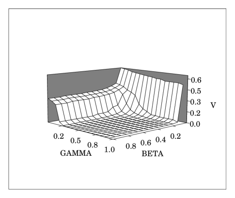
Figure 2: $V$ plotted as lines of constant vortex density. $V=0.4,0.3,0.2,0.1$, from left to right.

Figure 3: Surface plot of the vortex density, $V$, as measured on a $8^{4}$ lattice.

$V$ essentially vanishes in the Higgs phase and rises sharply across the phase boundary to a non-zero value in the Coulomb phase. Figure 4 shows separate “heating” and “cooling” runs at fixed $\beta=0.2$.

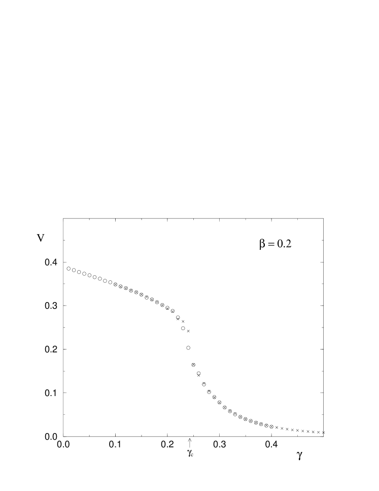
Figure 4: Measurements of $V$ on a $8^{4}$ lattice, at $\beta=0.2$. Crosses correspond to data taken with increasing $\gamma$ steps. Circles correspond to decreasing $\gamma$ steps.

The phase transition, given by the peak in the specific heat, is marked by the arrow at $\gamma_{\mathrm{c}}=0.24$. Statistical errors are of the size of the data points. The hysteresis in the data at the critical point appears indicative of the continuous (2nd order) phase transition there. Runs at other values of the couplings produced similar, excellent, agreement. Therefore, $V$ appears to be a good order parameter for the system.

To better understand the distribution of the vortices, a routine was written to measure the area of each connected vortex sheet. The results support the description of the phase transition given in section 2. Deep into the Higgs phase only small sheets are present, containing six or ten dual plaquettes each. As the system is moved towards the transition the average size of the clusters increases. Near the transition the clusters begin to coalesce into one large cluster, and the number of separate clusters drops dramatically. This occurs in the Higgs phase, before the phase boundary is reached. When the system reaches the Coulomb phase there is only a single large cluster, roughly the size of the lattice. If the system is heated further, the density of this cluster continues to increase.

In conclusion, the numerical simulations presented here seem to confirm the picture presented by the large $\gamma$ analysis of the theory. In the Higgs phase the vortex density is low and the area of each sheet is relatively small. In the Coulomb phase the vortex sheets are large and overlap, forming a single cluster of dual plaquettes. The abrupt change in the vortex density is coincident with the transition, given by the peak in the specific heat. Hence, the phase transition in the non-compact Abelian Higgs model, for $\lambda\to\infty$, appears to be driven by the condensation of vortex excitations.

The author would like to thank John B. Kogut for assistance with the Monte Carlo simulations and other helpful discussions. The author was supported in part by a GAANN fellowship.

Appendix

Here it is shown how to transform the Villain form of the partition function into equation (4). The steps are essentially the same as those used in analyzing the compact model [4]. For greater clarity we will suppress the spatial dependence of the fields. (See ref. [13] for a derivation using lattice differential forms.)

We start with

$$Z=\sum_{a_{\mu}=-\infty}^{\infty}\!\int_{-\infty}^{\infty}\mathrm{D}\!\chi\mathrm{D}\!A_{\mu}\,\mathrm{e}^{-{\beta\over 2}\sum(\epsilon_{\mu\nu\lambda\rho}\Delta_{\lambda}A_{\rho})^{2}-\gamma\sum(\Delta_{\mu}\chi-A_{\mu}+2\pi a_{\mu})^{2}}$$ (A.1)

and use the identity

$$\mathrm{e}^{-\textstyle{\kappa\over 2}x^{2}}=\sqrt{1\over{2\pi\kappa}}\int_{-\infty}^{\infty}\!\mathrm{d}\!y\,\mathrm{e}^{-{y^{2}\over{2\kappa}}+\mathrm{i}yx}$$ (A.2)

to rewrite each of the Gaussian integrals.

$$Z \sim \sum_{a_{\mu}=-\infty}^{\infty}\int_{-\infty}^{\infty}\mathrm{D}\!\chi\mathrm{D}\!A_{\mu}\mathrm{D}\!L_{\mu}\mathrm{D}\!S_{\rho\sigma}$$ (A.3)

$$\mbox{ }\mathrm{e}^{\sum\bigl{[}-{S_{\rho\sigma}^{2}\over{2\beta}}+\mathrm{i}S_{\rho\sigma}\epsilon_{\rho\sigma\mu\nu}\Delta_{\mu}A_{\nu}-{L_{\mu}^{2}\over{4\gamma}}+\mathrm{i}L_{\mu}(\Delta_{\mu}\chi-A_{\mu}+2\pi a_{\mu})\bigr{]}}.$$

Integrating over $\chi$ and $A_{\mu}$ gives

$$Z \sim \sum_{a_{\mu}=-\infty}^{\infty}\int_{-\infty}^{\infty}\mathrm{D}\!L_{\mu}\mathrm{D}\!S_{\rho\sigma}\delta(\Delta_{\mu}L_{\mu})\delta(L_{\mu}+\epsilon_{\mu\nu\rho\sigma}\Delta_{\nu}S_{\rho\sigma})$$ (A.4)

$$\mbox{ }\mathrm{e}^{\sum\bigl{[}-{S_{\rho\sigma}^{2}\over{2\beta}}-{L_{\mu}^{2}\over{4\gamma}}+2\pi\mathrm{i}L_{\mu}a_{\mu}\bigr{]}}.$$

The constraint imposed by $\delta(\Delta_{\mu}L_{\mu})$ can be removed by letting

$$L_{\mu}=\epsilon_{\mu\nu\rho\sigma}\Delta_{\nu}B_{\rho\sigma}.$$ (A.5)

The second constraint then becomes

$$\epsilon_{\mu\nu\rho\sigma}\Delta_{\nu}(B_{\rho\sigma}+S_{\rho\sigma})=0,$$ (A.6)

implying that

$$B_{\rho\sigma}+S_{\rho\sigma}=\Delta_{\rho}\psi_{\sigma}-\Delta_{\sigma}\psi_{\rho}.$$ (A.7)

We still must choose a gauge for $B_{\rho\sigma}$ to insure that $L_{\mu}$ is properly defined. The most convenient choice is to take $B_{\rho\sigma}+S_{\rho\sigma}=0$. The partition function is then

$$Z \sim \sum_{a_{\mu}=-\infty}^{\infty}\int_{-\infty}^{\infty}\mathrm{D}\!B_{\rho\sigma}$$ (A.8)

$$\mbox{ }\mathrm{e}^{-\textstyle{1\over{4\gamma}}\sum\bigl{[}(\epsilon_{\mu\nu\rho\sigma}\Delta_{\nu}B_{\rho\sigma})^{2}+m^{2}B_{\rho\sigma}^{2}+2\pi\mathrm{i}a_{\mu}(\epsilon_{\mu\nu\rho\sigma}\Delta_{\nu}B_{\rho\sigma})\bigr{]}},$$

with $m^{2}\equiv\textstyle{2\gamma\over\beta}$. Finally, integrating over $B_{\rho\sigma}$, we get the desired result

$$Z\sim Z_{o}\!\sum_{a_{\mu}=-\infty}^{\infty}\mathrm{e}^{-4\pi^{2}\gamma\sum J_{\mu\nu}(x)D(x-y;m^{2})J_{\mu\nu}(y)},$$ (A.9)

where $(-\Delta^{2}+m^{2})D(x-y;m^{2})=\delta_{xy}$ and $J_{\mu\nu}\equiv\epsilon_{\mu\nu\lambda\sigma}\Delta_{\lambda}a_{\sigma}$. $Z_{o}$ is the determinant given by setting all the $a_{\mu}=0$ in (A.8), and is completely analytic.

References

- [1] T. Banks, R. Myerson, and J. Kogut, Nucl. Phys. B129 (1977) 493.
- [2] T. A. DeGrand and D. Toussaint, Phys. Rev. D 22 (1980) 2478.
- [3] J. S. Barber and R. E. Shrock, Nucl. Phys. B257 (1985) 515.
- [4] M. B. Einhorn and R. Savit, Phys. Rev. D 17 (1978) 2583; Phys. Rev. D 19 (1979) 1198.
- [5] J. Ranft, J. Kripfganz, and G. Ranft, Phys. Rev. D 28 (1983) 360.
- [6] J.M.F. Labastida, E. Sanchez-Velasco, R. E. Shrock and P. Wills, Nucl. Phys. B 277 (1986) 393.
- [7] M. G. Amaral and M. E. Pol, Z. Phys. C 44 (1989) 515.
- [8] D. Callaway and R. Pertronzio, Nucl. Phys. B 277 (1986) 50; J. Jersak, in: Lattice Gauge Theory - A Challenge in Large-Scale Computing, eds. B. Bunk, K.H. Mütter and K. Schilling (Plenum Press, 1986) p.133; M. Baig, E. Dagotto, J. Kogut, and A. Moreo Phys. Lett. B 242 (1990) 444.
- [9] M. Baig, H. Fort, J. Kogut, and S. Kim, Phys. Rev. D 51 (1994) 5216.
- [10] M. E. Peskin, Ann. Phys. 113 (1978) 122.
- [11] C. Borgs F. Nill, J. Stat. Phys 47 (1987) 877.
- [12] H. B. Nielsen and P. Olesen, Nucl. Phys. B61 (1973) 45.
- [13] M.I. Polikarpov, U.-J. Wiese, M.A. Zubkov, Phys. Lett. B 309 (1993) 133; M. A. Zubkov and M. I. Polikarpov, JETP Lett. 57 (1993) 461.
- [14] A. K. Bukenov, U.-J. Wiese, M. I. Polikarpov, and Pochinskii, Phys. At. 56 (1993) 122.
- [15] J. Villain, J. Phys. (Paris) 36 (1975) 581.