UNIGRAZ- UTP- 26-02-96 Universality of the Ising model on sphere–like lattices

Abstract

We study the 2D Ising model on three different types of lattices that are topologically equivalent to spheres. The geometrical shapes are reminiscent of the surface of a pillow, a 3D cube and a sphere, respectively. Systems of volumes ranging up to O($10^{5}$) sites are simulated and finite size scaling is analyzed. The partition function zeros and the values of various cumulants at their respective peak positions are determined and they agree with the scaling behavior expected from universality with the Onsager solution on the torus ($\nu=1$). For the pseudocritical values of the coupling we find significant anomalies indicating a shift exponent $\neq 1$ for sphere–like lattice topology.

1 Motivation and introduction

Most of the Monte Carlo studies of spin models have been done on hypercubic lattices with periodic boundary conditions, i.e. with the topology of a torus. Recently, however, there has been a growing interest in the effect of other topologies. Some of that interest is motivated by the advance of quantum gravity models, some by problems related to the role of topological excitations of the particular system.

Various investigations [1–6] have been carried out on lattices topologically equivalent to the surface of a hypersphere in $D+1$ dimensions. On sphere–like surfaces a loop can be continuously contracted to a point: The fundamental homotopy group is trivial. This has immediate consequences for the dynamics of string–like objects like monopole loops (in 4D pure gauge theory with $U(1)$ gauge symmetry) or the boundaries of clusters in 2D spin models. We therefore might expect a different approach to the thermodynamic limit and different finite size corrections to scaling.

At first order phase transitions the phase mixture obtained in the thermodynamic limit may be influenced by local changes, like fixing one spin, or changing the boundary conditions. The critical exponents however, should not depend on such effects. At second order phase transitions one expects that the critical properties are not affected by boundary conditions or by whether one works on lattices with torus or spherical surface geometries if either becomes flat in the infinite volume limit. Such an assumption of universality should be tested in practical examples, which is one of the motivations for this work. Another question is whether the finite size scaling (FSS) ansatz is general enough to persist. The important leading terms and the corrections to them may have different size depending on the lattices and their topology as has been observed in the 4D and 2D studies.

The Ising model is explicitly solved for torus geometry [7] even on finite lattices [8, 9]. It has a well understood $2^{\mbox{\rm\footnotesize nd}}$ order phase transition. FSS of the bulk quantities is dominated by the leading term and provides a good example of the power of this method to determine critical indices.

Here we want to present a Monte Carlo study for the Ising model on different 2D lattices with the topology of the surface of a sphere: the surface of a 3D cube, a pillow–like structure and the cubic surface projected to a sphere. In all these cases we determine cumulants and partition function zeros on different lattice sizes in order to study the size dependence and FSS in detail. After the introduction of these geometries in sect.2, the simulation and multi–histogram analysis are discussed in sect.3 and the results in sect.4. We conclude that there are sizable differences to the usual results on torus–like lattices, but that universality prevails. Preliminary results of this work have been presented in [6].

2 Lattice geometry

The most straightforward approach to constructing a sphere–like lattice would be triangulation. We want to stay as close as possible to the original action, however. This is partly motivated by the related studies [1] and [5], where one wants to keep a 4-link plaquette structure. Also, two of the lattices studied here can be viewed at as combinations of the usual square lattices glued together at the boundaries; thus in the thermodynamic limit even the non–universal critical coupling ought to agree with that for torus geometry.

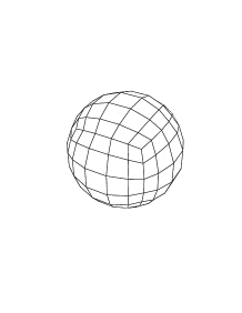
Figure 1: Lattices ${P\!I\,}$[6], ${S\!H\,}$[6] and $S$[6].

The torus is our reference geometry; in addition three other lattice geometries were used for our simulations (cf. fig. 1).

Torus ${T\!O\,[N]}$:

The solution for the Ising model on an $N\times N$ lattice with periodic b.c. is known [8, 9] and we will use this as the standard to compare our results with.

Pillow ${P\!I\,[N]}$:

This is the surface of a cube with $N\times N\times 2$ sites, where $N$ will be called the base length in the subsequent discussion. Basically it is made out of two $N\times N$ lattices glued together at the edges. The curvature is concentrated in the $4\times 2$ corners, elsewhere the lattice is locally flat. This lattice ${P\!I\,}$[N] has $2N^{2}$ sites and $4(N^{2}-1)$ links.

(Dual) Cube ${S\!H\,[N]}$:

This lattice is dual to the surface of a 3D cubic lattice of base length $N$. Each plaquette of the cubic surface is identified with a site of ${S\!H\,}$. This has the advantage, that each site has 4 links to nearest neighbors, like for the torus. The lattice has $6(N-1)^{2}$ sites and $12(N-1)^{2}$ links. The curvature is concentrated on the $8\times 3$ corner points.

Sphere ${S\,[N]}$:

That lattice is defined by the sites on the surface of a $N^{3}$ cube, projected onto the unit sphere. The site–link connectivity structure is identical to that of the cube’s surface, the only difference lies in weight factors in the action, to be discussed below. The lattice has $6(N-1)^{2}+2$ sites and $12(N-1)^{2}$ links.

The total energy (or action, if used in the context of quantum field theories) for the model is given by

$$E=-\sum_{x,\mu}w_{x,\hat{\mu}}s_{x}s_{x+\hat{\mu}}$$ (1)

where the sum runs over all links (at sites $x$ in directions $\hat{\mu}$). The spin variables $s_{x}$ have values $\in\mathbf{Z}(2)$. The weight factors $w_{x,\hat{\mu}}$ are equal to 1 for the torus and the lattice types ${P\!I\,}$ and ${S\!H\,}$. The partition function is determined by the sum

$$Z=\sum_{C}\exp{(-\beta E(C))}$$ (2)

over all spin configurations $C$.

For lattices ${P\!I\,}$ and ${S\!H\,}$ the curvature is concentrated around the corners. The deficit angle denotes the deviation of the sums of angles of plaquettes (or triangles) at a given site from the flat–space value $2\pi$. For ${P\!I\,}$ its value is $\pi/2$ on each of the $4\times 2$ corners, for ${S\!H\,}$ it is $\pi/6$ on each of the $8\times 3$ corners. It vanishes on all other sites, as it does on the torus: The lattices are flat almost everywhere. The total curvature on the sphere–like lattices therefore has the value $4\pi$ or Euler number 2, as compared to 0 for the torus. Euler’s relation for sphere–like lattices is $n_{s}+n_{p}-n_{l}=2$ ($n_{s}$, $n_{p}$, and $n_{l}$ denote the total number of sites, plaquettes and links, respectively) whereas for torus topology this sum is zero.

Both lattice types ${P\!I\,}$ and ${S\!H\,}$ can be imagined as built out of flat $N\times N$ pieces, glued together along their boundaries. The deviation from the torus shaped lattice thus disappears at least as fast as a boundary contribution $O(1/N)$. The contribution from the corners, where the curvature is concentrated, is suppressed $O(1/N^{2})$. We expect that, although not a universal quantity, the value of the critical coupling $\beta_{c}$ (in the thermodynamic limit) coincides with that for the torus.

In order to mimic a truly spherical lattice more closely, we also took the structure of a cubic surface lattice projected to the sphere as shown in fig. 1. Since the link connectivity structure does not change, the difference has to be expressed by modifying the weight factors accordingly. Christ et al. [10] discuss a possible definition for triangulated (random) surfaces, which obeys certain properties, that are necessary for the consistency of the continuum field theory at a second order phase transition.

Our lattices are built out of quadrangles and therefore we have to modify that method for the derivation of the weight factors. We start with the scalar continuum field theory with the Euclidean invariant kinetic term

$$\int d^{2}x\left(\partial_{\mu}\phi(x)\right)^{2}\quad.$$ (3)

(In fact, we can define the Ising model as a discretization of a scalar field theory in the limit of infinite quartic self coupling.) The discretization on a lattice replaces the derivative term by the nearest neighbor differences, $\partial_{\mu}\phi(x)\longrightarrow(\phi_{x+\hat{\mu}}-\phi_{x})/{l_{x,x+\hat{\mu}}}$, where $l_{x,y}$ denotes the distance between the neighboring two points. The area differential $d^{2}x$ has to be replaced by an area element $A_{x,\hat{\mu}}$ assigned to each lattice link (or site term). The discretized kinetic term then leads to the link term of the lattice action (1), with the weight factor $w_{x,\hat{\mu}}=2A_{x,\hat{\mu}}/l_{x,x+\hat{\mu}}^{2}$.

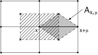
Figure 2: The rectangular hatched area as attributed to the site $x$ is defined by the dual sites (indicated by crosses) and is proportional to the shaded area $A_{x,\hat{\mu}}$ that corresponds to the link from $x$ to $x+\mu$.

The total lattice volume has to be split into lattice area elements attributed to the link contributions. These lattice area elements are constructed with help of the dual lattice, where each site may be defined as the barycenter of the plaquettes of the original lattice (cf. fig. 2). Links of the dual lattice are drawn between sites corresponding to neighboring plaquettes. Each link on the original lattice corresponds exactly to one link of the dual lattice.

For simplicity we make two approximations:

• We assume that all quadrangles are flat; in reality the four corners are not co–planar. In the thermodynamic limit the lattice becomes locally flat and the error vanishes.

• We neglect angular distortions and approximate each quadrangle by a rectangle; this allows us to write the area assigned to a lattice link $x$ as the product of the lengths of the dual link with that of the link itself, $A_{x,\hat{\mu}}=\frac{1}{2}\;l^{\prime}_{x,\hat{\mu}}\times l_{x,\hat{\mu}}$. The error introduced due to this approximation does not vanish in the thermodynamic limit and introduces slight distortions from the regular spherical surface. However, the curvature is still smeared out over the whole lattice, although somewhat non–uniformly. As will turn out later, that appears to be no serious problem for the finite size analysis.

This way the total lattice volume is distributed over all links.

With these approximations we find that the weight factors for the lattice geometry $S[N]$ are just the ratio of dual link length to the link length

$$w_{x,\hat{\mu}}\equiv l_{x,\hat{\mu}}^{\prime}/l_{x,\hat{\mu}}$$ (4)

equivalent to the factor suggested in [10] for triangulations.

For this particular sphere–like lattice we do not expect, that the thermodynamic limit value of the critical coupling is identical to that of the torus. Since we have introduced a change of the action affecting all links, $\beta_{c}$ will be renormalized. Still we expect universal behavior of the critical exponents, to be checked numerically.

The computer programs use index tables to deal with the lattice geometry. For the lattices $S[N]$ the weight factors are precalculated and tabulated. In our discussions we will refer to the lattice volume

$$V=\sum_{x,\mu}w_{x,\hat{\mu}}$$ (5)

as the typical size quantity. For lattices ${T\!O\,}$, ${P\!I\,}$ and ${S\!H\,}$ this is just the number of links. A length scale may be defined as $L\equiv\sqrt{V/2}$, such that its value is $N$ for a torus ${T\!O\,}[N]$.

In another study of the Ising model [3] regular honeycomb lattices folded to tetrahedron shapes have been used. There it was possible to obtain series expansions as well as Monte Carlo results. In [4] the Ising model was studied with Monte Carlo methods on triangulated random lattices with sphere–like topology. We compare these results with ours in the section 4.

3 Simulation details

In the Monte Carlo simulation we studied lattices with the base length $N=$ 16, 32, 64 and 128. (The torus results were determined up to $N=256$.) The lattices have the volumes given in table 1.

Base Length $N$	$T\!O\,$	$P\!I\,$	$S\!H\,$	$S$
16	512	1020	2700	2724.8
32	2048	4092	11532	11650.0
64	8192	16380	47628	48147.0
128	32768	65532	193548	195726.9

Table 1: The volumes $V$ as defined in the text; the equivalent linear extent $L=(V/2)^{\frac{1}{2}}$ ranges from 16 (for the torus) up to 313 (for the sphere).

For the updating of the spins we used the Swendsen–Wang cluster algorithm [11]. For each lattice size the bulk energy histograms were determined for various values of the coupling and then combined with help of the Ferrenberg–Swendsen multihistogram technique [12]. This leads to an optimal estimator for the distribution densities $\rho_{L}(E)$ for the partition function

$$Z_{L}(\beta)=\sum_{E}\rho_{L}(E)\exp(-\beta E)$$ (6)

and allows to determine various moments $\langle f(E)\rangle$. Of course the statistical accuracy deteriorates when one evaluates these quantities outside the domain of $\beta$–values, where one determined the histograms. Suitable overlap between the individual histograms is necessary for a reliable application of the method. We determined only the energy histograms and analyzed only observables in the even sector of the model and not the observables that involve the magnetization.

We measured the specific heat, the Challa–Landau–Binder cumulant [13] and another $4^{\mbox{\footnotesize th}}$ order cumulant suggested by Binder (cf. the review [14]):

$$c_{V}(\beta,L) = ~{}~{}\frac{1}{V}\langle(E-\langle E\rangle)^{2}\rangle\;,$$ (7)

$$V_{CLB}(\beta,L) = -\frac{1}{3}\frac{\langle(E^{2}-\langle E^{2}\rangle)^{2}\rangle}{\langle E^{2}\rangle^{2}}\;,$$ (8)

$$U_{4}(\beta,L) = \frac{\langle(E-\langle E\rangle)^{4}\rangle}{\langle(E-\langle E\rangle)^{2}\rangle^{2}}\;.$$ (9)

The positions and values of their respective extrema are used for the FSS analysis.

Eq. (6) defines implicitly an analytic continuation to complex values of $\beta$ not too far away from the real axis. Therefore it is possible to determine the nearby zeros of the partition function [15] in the complex $\beta$–plane, the so–called Fisher zeros [16]. As will be demonstrated below, in particular the imaginary part of the zero closest to the real axis provides a high quality estimator for the critical exponent $\nu$ with small corrections to the leading FSS behavior (cf. [17] for a recent high statistics study of the Ising model in 4D, where it was possible to identify the logarithmic corrections to scaling on basis of the Lee–Yang singularities [15]). So real and imaginary parts of the closest Fisher zeros provide further (even) observables.

For each lattice size we simulated the system at up to 20 different values of $\beta$ between 0.41 and 0.47. The integrated autocorrelation times for the energy varied between $\tau\approx 3-7$. For each size we produced between 2 and $5\times 10^{6}$ independent configurations. The errors were estimated with the jackknife algorithm, i.e. from the variation of the results for the analysis of subsamples of the raw data.

Throughout the discussion of the data we use $L\equiv\sqrt{V/2}$. The fit quality is expressed through the goodness of fit parameter $Q$.

4 Results and analysis

4.1 Finite size scaling and topology

From the usual scaling hypothesis [18, 19] one expects for the singular part of the free energy density the scaling behavior

$$f(\tau,L)=L^{-1/D}f(\tau L^{1/\nu},1)\;,$$ (10)

where $\tau=(1-\beta/\beta_{c})$ denotes the reduced coupling and $L$ is the length scale. From this one derives the scaling behavior of the cumulants. At a second order phase transition we expect (for $D=2$)

$$C_{max}(L) \simeq \left\{\begin{array}[]{ll}L^{\alpha/\nu}&(\mbox{for~{}}\alpha>0)\\ O(\ln L)&(\mbox{for~{}}\alpha=0)\end{array}\right.$$ (13)

$$V_{CLB,min}(L) \simeq \left\{\begin{array}[]{ll}L^{\alpha/\nu-2}&(\mbox{for~{}}\alpha>0)\\ L^{-2}\ln L&(\mbox{for~{}}\alpha=0)\end{array}\right.$$ (16)

$$U_{4,min}(L) \simeq \left\{\begin{array}[]{ll}O(1)+O(L^{-\alpha/\nu})&(\mbox{for~{}}\alpha>0)\\ O(1)+O(1/\ln L)^{2}&(\mbox{for~{}}\alpha=0)\end{array}\right.$$ (19)

$$\mbox{Im}\;z_{0}(L) \simeq L^{-1/\nu}$$ (20)

$$\beta_{c}(L)-\beta_{c} \simeq L^{-\lambda}$$ (21)

with Josephson’s law $\alpha=2-D\nu$. The asymptotic value of $U_{4}$ depends on the details of the distribution density $\rho(E)$ and is e.g. 3 for a Gaussian distribution. For the Ising model the Onsager solution gives $\nu=1$ and $\alpha=0$.

We denote by $\beta_{c}(L)$ our definitions for pseudocritical points: The positions of the extrema in the cumulants. The so–called shift–exponent $\lambda$ is for many models equal to $1/\nu$, but not necessarily so in general; this relation is not a necessary conclusion of FSS (cf. the discussion in [19]). We return to this issue in the discussion of the results.

A priori we know nothing about the absolute size of the multiplicative coefficients in the scaling formulas. They depend on the details of the lattice geometry and topology and on the boundary conditions.

The FSS behavior comes from the rescaling properties of the bulk quantities. The effect of changing the boundary properties may be responsible for further contributions. The non–homogeneous distribution of the curvature in our lattices ${P\!I\,}$ and ${S\!H\,}$ might also be responsible for additional (constant) terms in the total free energy.

Actually, since the total curvature is an invariant, there may be another contribution, which — relative to the bulk contribution $O(V)$ — becomes irrelevant in the thermodynamic limit. It has been shown [20], that the total free energy for finite 2D systems with non–singular metric and smooth boundaries has at criticality (in addition to boundary terms $O(L)$) an asymptotic contribution proportional to $\ln L$. The proportionality constant is a product of the central conformal charge and the Euler number (vanishing for the torus). Thus this contribution depends only on the topology of the system, not on the shape of the boundary.

All these contributions to the free energy are suppressed $O(1/L^{2})$ or $O(\ln{L}/L^{2})$ relative to the leading term. In the absence of a strict theory we therefore might expect corresponding additive corrections terms in the FSS relations (13) – (21).

4.2 Cumulant values and partition function zeros

The values of the cumulants at their respective pseudocritical points provide information on the critical exponents according to (13) – (19). As discussed, they may have geometry dependent corrections. However, in our data we find qualitatively excellent agreement with the scaling of the torus–results and no significant indication of geometry–corrections.

Fig. 3 shows that the specific heat scales with $\ln L$, as expected for $\alpha=0$. A power law fit gives a value for $\alpha$ compatible with 0 and has a larger $\chi^{2}$: The logarithmic behavior is preferred.

Comparing the results for the higher order cumulants $V_{CLB}$ and $U_{4}$ we also find excellent agreement with the torus results, if compared at the corresponding scales $L$, and with the expected scaling behavior for $\alpha=0$ according to (16) – (19). In particular the results for $V_{CLB}$ lie on top of a common curve for all geometries.

The finite size dependence of the positions of the partition function zeros confirms this observation. In fig. 4 the nearest Fisher zeros for sphere–like lattices are compared with those for toroidal lattice. The real part is substantially closer to the thermodynamic limit. Its scaling properties are discussed below together with the pseudocritical points derived from the cumulants.

The imaginary part of the closest Fisher zero appears to profit from the smallness of the deviation of the real part from the thermodynamic value. The log–log plot (fig. 5) demonstrates the excellent scaling signal and a fit of the form

$$\mbox{Im}\;z_{0}(L)=aL^{-1/\nu}$$ (22)

gives $\nu=0.9964(46)$ (goodness of fit $Q=0.39$) for ${P\!I\,}$, $\nu=0.9975(57)$ ($Q=0.77$) for ${S\!H\,}$ and $\nu=1.0023(54)$ ($Q=0.12$) for $S$ lattices. For all these lattices the result is in perfect agreement with the value $\nu=1$ of the toroidal lattice.

We conclude, that the imaginary part of the first partition function zero is an optimal observable for extracting the critical exponent $\nu$. It appears to be least affected by correction to scaling due to lattice topology and boundary effects.

In this light the excellent scaling behavior of the specific heat should not be too surprising, since the peak value is directly related to the vicinity of the closest Fisher zero. Since the partition function is proportional to the product of all zeros,

$$Z\propto\prod_{i}(\beta-z_{i})$$ (23)

the specific heat includes for its singular part the contribution

$$\sum_{i}\frac{1}{(\beta-z_{i})^{2}}\;.$$ (24)

The closest zero therefore contributes a term $\propto(\mbox{Im}\;z_{0})^{-2}$ to the peak value of $c_{V}$ [17].

The fact, that the closest zero approaches the real axis (with increasing lattice size) almost perpendicular is also clearly exhibited by the shape of the specific heat itself. In fig. 6 we compare the torus results with those for the cubic surface lattices for equivalent lattice volumes. The approach to the infinite volume case (Onsager solution) is in a much more symmetric way than for the torus lattice.

4.3 Pseudocritical points

We discuss here the pseudocritical values derived from

• the peak positions of the specific heat,

• the minima positions of the other cumulants $V_{CLB}$ and $U_{4}$,

• the real part of the position of the closest zero in the complex $\beta$–plane.

For the lattice geometries ${P\!I\,}$ and ${S\!H\,}$ we expect (see the discussion in sect. 2) that in the thermodynamic limit the critical values $\beta_{c}$ coincide with those of the torus, and we therefore present these results in direct comparison. For the lattice type $S$ the asymptotic value of the critical coupling will be somewhat different and we discuss these results separately.

4.3.1 ${P\!I\,}$  and ${S\!H\,}$  lattices

It turns out, that both lattice geometries have very similar behavior and agree (except for the smallest lattice ${P\!I\,}[16]$) even numerically with each other, if compared at corresponding volumes.

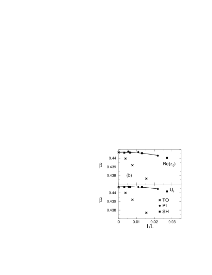
Figure 7: Results for the pseudocritical coupling vs. $L$ for (a) the specific heat $c_{V}$ and $V_{CLB}$, (b) the real part of the closest partition function zero and $U_{4}$, for pillow, dual cube and torus type lattices. The curves are fits according to (25) for the pillow and cubic surface lattices as described in the text.

As fig. 7 clearly exhibits, there is an obvious difference in the FSS behavior compared to the usual torus results. The overall size of the corrections to the thermodynamic value of the critical coupling are much smaller for the sphere–like lattices. The leading FSS behavior of $\beta_{c}(L)$ for large $L$ should follow (21). For the Ising model on a torus the shift exponent is $\lambda=1/\nu=1$ [9]. This leading behavior linear in $1/L$ is evident in the figure. However, for ${P\!I\,}$ and ${S\!H\,}$ another effect seems to blur this picture: A possible (but clearly very small) linear term is dominated by contributions nonlinear in $1/L$.

As discussed in [19] the leading linear term may vanish even for $N\times M$ torus geometry, depending on the ratio $N/M$. In particular it vanishes in the limit $M\to\infty$, where the leading behavior becomes $O(\ln L/L^{2})$ [9]. There are also other specific models and cases, where $\lambda\neq 1/\nu$ [19]. As mentioned below (21) also the topology may give rise to additional terms [20] in the free energy (per unit volume) proportional to the Euler number and to $O(\ln L/L^{2})$; it is unclear how these affect the pseudocritical points in our particular situation.

This observation, that the dominating behavior appears to be non–linear in $1/L$, was also made in a study of the Ising model for a honeycomb lattice on a tetrahedron surface [3]. Both, series and Monte Carlo results led to a value $\lambda=1.745(15)$ [3]. The value of $\nu$ obtained there from the correlation length and the specific heat agreed with the Onsager value.

We therefore fit our data for the pseudocritical points to

$$\beta_{c}(L)-\beta_{c} = aL^{-1}+bL^{-\lambda}\quad,$$ (25)

$$\beta_{c}(L)-\beta_{c} = aL^{-1}+bL^{-2}\ln{L}\quad,$$ (26)

with the Onsager value for $\beta_{c}=\frac{1}{2}\ln{(1+\sqrt{2})}$.

The data for each of the 4 definitions of pseudocritical coupling (from $c_{V}$, $V_{CLB}$, $U_{4}$ and $\mbox{Re}\;z_{0}$) appears to be consistent for both geometries ${P\!I\,}$ and ${S\!H\,}$. We therefore use one set of parameters $a$ and $b$ different for each definition but identical for the two geometries. The value of $\lambda$ is assumed to be universal for all definitions and both geometries. We fit to data for $N\geq 32$. The results according to (25) are given in table 2 and are plotted in fig. 7: they fit the data perfectly with a $\chi^{2}/d.f.\simeq 1.2$ $(Q=0.26)$.

Lattice	$\lambda$	Par.	$c_{V}$	$V_{CLB}$	$U_{4}$	Re $z_{0}$
${P\!I\,}$,${S\!H\,}$	1.76(7)	$a$	0.002(4)	0.000(13)	-0.011(5)	0.009(10)
		$b$	-0.83(18)	-4.29(96)	-0.37(13)	-0.45(24)
$S$	1.71(10)	$a$	0.028(10)	0.025(28)	0.032(11)	0.029(11)
		$b$	-0.62(13)	-3.34(86)	-0.24(14)	-0.29(13)

Table 2: Scaling law coefficients $a$, $b$ and exponent $\lambda$ for the various lattice geometries. Fits are according to (25) to data for $N=32\ldots 128$ for ${P\!I\,}$ and ${S\!H\,}$ and $N=16\ldots 128$ for $S$

As expected from looking at the data we find only a small contribution to the term $O(1/L)$, compatible with zero for all observable except for $U_{4}$. Removing this term altogether seems conceivable, although $\chi^{2}$ is quadrupled in this case. The second term clearly dominates. However, the resulting value $\lambda=1.76(7)$, although consistent with the results for the tetrahedron [3], is not stringent. In fact, allowing for the second ansatz (26) give almost the same fit quality and would be indistinguishable in the figure. Also fixing $\lambda$ to a value $2$ is still compatible with the data.

We conclude that we are in a situation where a possible leading FSS term $O(1/L)$ has an (almost or completely) vanishing coefficient and the subleading terms dominate. This resembles the Ising model on a cylinder with infinite extension in one direction. It cannot be decided, whether the corresponding term is of form (25) or (26).

4.3.2 Spherical surface lattices

Now we turn to the approximate spherical surface topology ($S$). Whereas for the pillow and cubic surface lattices the curvature is concentrated in 8 or 24 points here it is more or less uniformly distributed among all sites of the lattice. The total curvature (the Euler number) remains constant.

In fig. 8 the peak positions of the specific heat and the other cumulants are plotted together with fitted curves according to (25). Here $\beta_{c}$ is a free parameter, otherwise we follow the procedure discussed above, i.e. one common value of $\lambda$ but different parameters $a$ and $b$ depending on the observable. Since we have fewer data we include the data from the smaller lattices with $N=16$. This is also justified by the overall smaller deviations from the asymptotic value.

The resulting values are also given in table 2. We find a behavior in agreement with the other sphere–like lattices. The contribution of the term $O(1/L)$ is again very small and the non–linear term dominates again. The overall variation of the pseudocritical points with $L$ is for most observables smaller than for the other lattice geometries. The fitted critical temperature is $\beta_{c}=0.43883(3)$ with a $\chi^{2}/d.f.\simeq 0.5$ ($Q=0.81$). The value of $\lambda=1.71(10)$ is consistent.

Again the fit to (26) gives results of comparable quality and corresponding curves would be indistinguishable in the figure.

5 Conclusion

We have performed a high statistics Monte Carlo study of the Ising model on lattices of various size and different shapes, all with sphere–like topology. Our FSS analysis led to the following conclusions.

• We have found explicitly, that the Ising model on a spherical surface topology lies in the same universality class as the planar Ising model with periodic boundary conditions — topologically the surface of a torus. Our results demonstrate that universality holds, independent of the lattice geometry. This agrees with similar conclusions obtained for tetrahedral lattices [3] and random lattices [4] of sphere–like topology.

• However, some observables are not well suited to find the expected leading FSS behavior. Different observables vary in their sensitivity. Of the studied quantities (in the even sector of the Ising model) we find that the imaginary part of the Fisher zero closest to the real axis has the smallest (in fact: not identifiable within our accuracy) deviations from the leading FSS behavior. Related to this quantity, also the peak value of the specific heat scales according to the FSS formulas with the Onsager values for the critical exponents without further (identifiable) corrections. The values of the other cumulant have larger statistical errors but are also in agreement with the torus results.

• The change in the topology class influences the size of the FSS contributions. This appears to affect in particular the pseudocritical points. We find no significant contribution of $O(1/L)$, which is the dominant FSS term for the torus pseudocritical points (with a shift exponent $\lambda=1/\nu=1$). Instead we find that the FSS behavior is dominated by a term $O(L^{-\lambda})$ with a mean value $\lambda\simeq 1.74(6)$ (averaging the results for ${P\!I\,}$, ${S\!H\,}$ and $S$). A compatible value was obtained in an independent study for tetrahedral lattices [3]. The behavior seems to be universal for all sphere–like lattices, independent of the details of the geometry. This contribution is also consistent with a term $O(\ln L/L^{2})$; such a term describes the FSS of the specific heat peak position for the Ising model in cylinder geometry [9]. It also has been argued, that a term of that kind contributes to the free energy per unit volume for systems with non–zero Euler number [20]. Unfortunately this implies that none of these observables is qualified to derive the critical exponent $\nu$.

• In general we find that the studied sphere–like lattices have smaller corrections to the infinite volume behavior than one observes for the torus (i.e. periodic boundary conditions). The approach to the thermodynamic shapes is faster and in a more symmetric way.

• Our analysis of the Fisher zeros of the partition function is consistent with this picture. With increasing size the closest zero approaches the real axis almost perpendicular. (Note, that this behavior is a finite size behavior and is not identical to the asymptotic impact angle – defined e.g. as the angle between the first and second zero). The results for the spherical surface geometry appear to be closest to the thermodynamic behavior in general. For different lattice (sphere–like) geometries the FSS behavior is consistent if one chooses the size variable $L=\sqrt{V/2}$, where $V$ is the number of links. This choice appears to be preferable over the base length $N$.

In general our conclusion are consistent with other results on sphere–like lattices for the Ising model [3, 4] and with similar observations in other models [6], also in higher dimensional lattices [2].

How can one explain the more symmetric and seemingly faster approach to the thermodynamic limit, that occurs for the sphere–like lattices as compared to the torus? One may argue, that on the 2D torus there are two globally distinguished directions. As soon as the correlation length $\xi$ approaches some fraction of the linear size, the system notices the loss of its rotational invariance. Larger clusters may then span in the two distinguished directions of the lattice. On sphere–like surfaces (although there is local orientation) there are no globally distinguished directions. Rotational invariance holds to a larger extent and the behavior of the finite system is more symmetric around the critical point.

Acknowledgment

We are most grateful to J. Jersák, M. Lüscher and T. Neuhaus for many helpful suggestions and discussions. We appreciate stimulating conversations with H. Gausterer, A. Jakovac and W. Janke.

Figure 3: Specific heat peak values vs. $\ln L$ for lattices ${P\!I\,}$, ${S\!H\,}$, ${T\!O\,}$ and $S$. Here and in all the other figures the error bars are smaller than the symbols.

Figure 4: (a) Position of the partition function zero closest to the real axis in the complex $\beta$ plane for different lattices.The numbers indicate the base length $N$. The real part of the zeros are closer to their thermodynamic value for the sphere–like lattices than for the torus. In (b) we plot the results for the spherical surface lattices $S$.

Figure 5: Plot of $\ln(\mbox{Im}\;z_{0})$ vs. $\ln L$; the fit represents the leading FSS behavior.

Figure 6: Specific heat per unit volume vs. $\beta$ for ${T\!O\,}[37]$ and ${S\!H\,}[16]$; these lattices of similar volume are compared to the Onsager solution. One finds that the curve for the ${S\!H\,}$ lattice is more symmetric around $\beta_{c}$ than for the ${T\!O\,}$.

Figure 8: Peak positions of the cumulants on spherical surface lattices $S$. One can clearly see, that $\beta_{c}$ differs from the critical temperature on the torus $\beta_{c,TO}\approx 0.44068$. The curves are from fits to (25.) The error bars are smaller than the symbols.

References

- [1] C. B. Lang and T. Neuhaus, Nucl. Phys. B 431, 119 (1994).
- [2] J. Jersák, C. Lang, and T. Neuhaus, Nucl. Phys. B (Proc. Suppl.) 42, 672 (1995).
- [3] O. Diego, J. González, and J. Salas, J. Phys. A 27, 2965 (1994).
- [4] C. Holm and W. Janke, FUB-HEP 18/95, KOMA-95-81, hep-lat/9512002 to appear in Nucl. Phys. B (Proc. Suppl.) (1996).
- [5] H. Gausterer and C. B. Lang, Nucl. Phys. B455, 785 (1995).
- [6] C. Hoelbling, A. Jakovac, J. Jersák, C. B. Lang and T. Neuhaus, preprint UNIGRAZ-UTP-070995, hep-lat/9509009, to appear in Nucl. Phys. B (Proc. Suppl.) (1996).
- [7] L. Onsager, Phys. Rev. 65, 117 (1944).
- [8] B. Kaufman, Phys. Rev. 76, 1232 (1949).
- [9] A. E. Ferdinand and M. Fisher, Phys. Rev. 185, 832 (1969).
- [10] N. H. Christ, R. Friedberg, and T. D. Lee, Nucl. Phys. B210 [FS6], 337 (1982).
- [11] R. H. Swendsen and J.-S. Wang, Phys. Rev. Lett. 58, 86 (1987).
- [12] A. M. Ferrenberg and R. H. Swendsen, Phys. Rev. Lett. 61, 2635 (1988), Err., ibid. 63, 1658 (1989); ibid., Phys. Rev. Lett. 63, 1195 (1989).
- [13] M. S. S. Challa, D. P. Landau, and K. Binder, Phys. Rev. B 34, 1841 (1986).
- [14] K. Binder, in Computational Methods in Field Theory, Lecture Notes in Physics 409, edited by H. Gausterer and C. B. Lang (Springer-Verlag, Berlin, Heidelberg, 1992), p. 59.
- [15] C. N. Yang and T. D. Lee, Phys. Rev. 87, 404 (1952).
- [16] M. E. Fisher, in Lectures in Theoretical Physics, edited by W. E. Brittin (Gordon and Breach, New York, 1968), Vol. VIIC, p. 1.
- [17] R. Kenna and C. B. Lang, Nucl. Phys. B 393, 461 (1993), Err. ibid. B 411, 340 (1994); Phys. Rev. E49, 5012 (1994).
- [18] M. E. Fisher, in Critical Phenomena, Proc. of the 51th Enrico Fermi Summer School, Varena, edited by M. S. Green (Academic Press, New York, 1972). M. E. Fisher and M. N. Barber, Phys. Rev. Lett. 28, 1516 (1972). E. Brézin, J. Physique 43, 15 (1982). J. L. Cardy, in Finite–Size Scaling, edited by J. L. Cardy (North-Holland, Amsterdam, 1988), p. 1.
- [19] M. N. Barber, in Phase Transitions and Critical Phenomena, Vol. 8, edited by C. Domb and J. Lebowitz (Academic Press, New York, 1983), Vol. VIII, Chap. 2, p. 104.
- [20] J. L. Cardy and I. Peschel, Nucl. Phys. B300[FS22], 377 (1988).