QCD Function with Two Flavors of Dynamical Wilson Fermions
March 22, 1996)
Abstract
We test the asymptotic scaling behavior of state-of-the-art simulations of QCD with two flavors of light Wilson fermions. This is done by matching and masses on lattices of size and . We find that at matching is not possible over a range extending down to . The large lattice data at matches the small lattice values at leading to a shift , considerably larger than the perturbative prediction of . In both cases we conclude that the simulations are very far from the asymptotic scaling region.
1 Introduction
Assuming that a universal continuum limit of lattice qcd exists, measurements of some physical observable , such as a hadron mass, in a Monte Carlo computation will not depend on the details of the lattice discretization if the lattice spacing is small enough. The value of the observable, , obtained by numerical calculation in lattice qcd with Wilson fermions, depends only on the parameters appearing in the lattice action: the gauge coupling and the hopping parameter . The dimensionless quantity has been related to the dimensionful observable by multiplying by the appropriate power of the lattice spacing . As we approach the continuum limit the fact that is independent of is expressed by the renormalization group equation
where
The derivatives with respect to are taken at “constant physics.” As we have two independent relevant parameters we require two independent physical observables to use as renormalization conditions to fix these parameters; and should, of course, be independent of the choice of renormalization conditions.
In a perturbative expansion of about only the first two terms are independent of the details of the lattice regularization scheme. When the higher order terms are negligible one generally speaks of being in the asymptotic scaling regime. The aim of this work is to determine, for the realistic case of qcd with two flavors of light Wilson fermions, how close present simulations are to this asymptotic scaling regime.
In numerical simulations it is impractical to determine the -function, which correspond to an infinitesimal change of scale, directly. Rather we work with a finite change of scale. We consider two lattices, with sites in each direction and with lattice spacing , and with sites in each direction and lattice spacing . By fiat we assert that and represent the same physical volume, thus .
If we select some set of physical observables we have
where is the dimension of and is the corresponding dimensionless function measured on the lattice. In the continuum limit all these observables must become independent of the lattice, so for the two different lattices
We define the quantities
to be the change in the couplings needed to compensate for this change in the cutoff.
2 The -function
We expect the -function to become independent of in the continuum and chiral limits.111If we use continuum perturbation theory with dimensional regularization and the minimal subtraction renormalization scheme, then the BRS identities insure that all divergences are logarithmic, and thus must be independent of the quark mass. From this we may conclude that in the vicinity of the chirally symmetric continuum limit any dependence of the -function must arise from irrelevant lattice operators and be suppressed by some power of the lattice spacing.
The -function at fixed is defined by , and the two universal terms from perturbation theory are where
for qcd with flavors of light fermions.
The solution of these equations, expressed in terms of , is
after evaluating the integral we find that
which is the perturbative prediction for the change in needed to effect a change in scale by a factor .
has been thoroughly studied for pure gauge theory with the Wilson action (see [1] and references therein) and exhibits the well-known dip around . For qcd with dynamical fermions we are unaware of recent studies of . For staggered fermions, Blum et al. [2], determined the -function, needed for the computation of the equation of state for finite temperature qcd, from fits to hadron masses obtained at different couplings, and hence different lattice scales. They found significant deviations from asymptotic scaling that again would lead to a dip in .
3 Results
The -function for two flavors of Wilson fermions was computed earlier by some of us [3, 4]. The physical observables used for that purpose were and several Creutz ratios of Wilson loops.
The main conclusion then was that perturbative scaling was only expected to occur for . In those simulations the -like object was heavy, and it was thought at the time that this may have hidden the effects of the dynamical fermions in the system. Simulations with smaller are thus needed to clarify the issue.
In this work we concentrated on data available on lattices of size with two flavors of Wilson fermions with parameters and results shown in Table 1 [5, 6]. These were matched using lattices with the parameters and results for the interesting parameter region shown in Table 2.
| 5.3 | 0.1670 | 484 | 5 | 0.4540(20) | 0.6350(20) | 0.9620(40) | 0.715(5) | 0.4719(29) |
| 5.3 | 0.1675 | 417 | 3 | 0.3120(40) | 0.5230(40) | 0.7660(90) | 0.596(15) | 0.4073(71) |
| 5.5 | 0.1596 | 400 | 5 | 0.3754(27) | 0.4947(78) | 0.7644(48) | 0.759(11) | 0.4911(36) |
| 5.5 | 0.1600 | 400 | 5 | 0.3262(17) | 0.4606(28) | 0.7106(91) | 0.708(4) | 0.4591(57) |
| 5.5 | 0.1604 | 669 | 3 | 0.2666(20) | 0.4208(55) | 0.6326(56) | 0.634(8) | 0.4215(48) |
| 4.8 | 0.1890 | 130 | 0.6681(41) | 0.964(12) | 0.964(12) | 0.678(16) | 0.4038(51) |
|---|---|---|---|---|---|---|---|
| 4.8 | 0.1900 | 170 | 0.5814(35) | 0.897(7) | 1.522(26) | 0.6480(54) | 0.3820(64) |
| 4.8 | 0.1905 | 109 | 0.5110(48) | 0.896(28) | 1.362(26) | 0.571(19) | 0.3753(65) |
| 4.9 | 0.1840 | 189 | 0.7826(28) | 1.013(5) | 1.783(36) | 0.7722(36) | 0.4390(88) |
| 4.9 | 0.1845 | 190 | 0.7520(23) | 0.988(5) | 1.714(20) | 0.7609(33) | 0.4388(49) |
| 4.9 | 0.1850 | 110 | 0.6808(46) | 0.928(5) | 1.549(13) | 0.7334(44) | 0.4396(40) |
| 4.9 | 0.1855 | 272 | 0.6491(40) | 0.930(7) | 1.660(57) | 0.6982(63) | 0.391(13) |
| 4.9 | 0.1860 | 200 | 0.5636(47) | 0.872(10) | 1.451(31) | 0.6467(88) | 0.3886(88) |
| 4.9 | 0.1865 | 150 | 0.5018(59) | 0.852(20) | 1.55(11) | 0.590(13) | 0.324(22) |
| 4.9 | 0.1870 | 70 | 0.4981(65) | 0.816(20) | 1.395(23) | 0.611(15) | 0.3572(81) |
| 4.95 | 0.1815 | 80 | 0.8083(37) | 1.003(6) | 1.693(19) | 0.8059(44) | 0.4775(47) |
| 5.0 | 0.1800 | 30 | 0.7734(85) | 0.990(14) | 1.690(36) | 0.781(11) | 0.4578(95) |
| 5.0 | 0.1810 | 150 | 0.6321(53) | 0.875(7) | 1.462(19) | 0.7228(53) | 0.4325(65) |
| 5.0 | 0.1815 | 270 | 0.5145(83) | 0.814(9) | 1.342(19) | 0.632(12) | 0.3834(77) |
A preliminary report on this work was presented in [7].
The values of were chosen for hadron spectrum and other calculations largely based on the assumption that the presence of two fermion flavors renormalizes downwards by about from its quenched value, and thus we may not be far from the perturbative scaling regime at these parameter values.
For our test of scaling we used two hadron masses, and , as observables for matching with similar data generated on lattices of size at values of ranging from down to and many values.
The simulations used step sizes from to to insure a reasonable acceptance rate. The conjugate gradient residual used for the molecular dynamics steps was . Hadron measurements were made every trajectories. We found integrated autocorrelation times were typically of this order.
Quark propagators with wall sources and point sinks were computed in Coulomb gauge on time slices and . We determined the meson masses by a correlated single state cosh fit to two correlation functions with interpolating fields and ; our baryon correlation functions used only one interpolating field. The covariance and errors were determined via the bootstrap method. Fits were made through the center of the lattice with a starting time slice determined by the criterion , where is the number of degrees of freedom for a fit of mass . In all cases , the 1 standard deviation confidence level, was greater than .
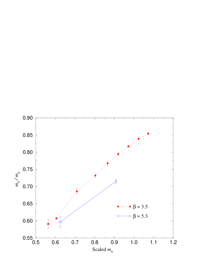
3.1 Non-Matching at
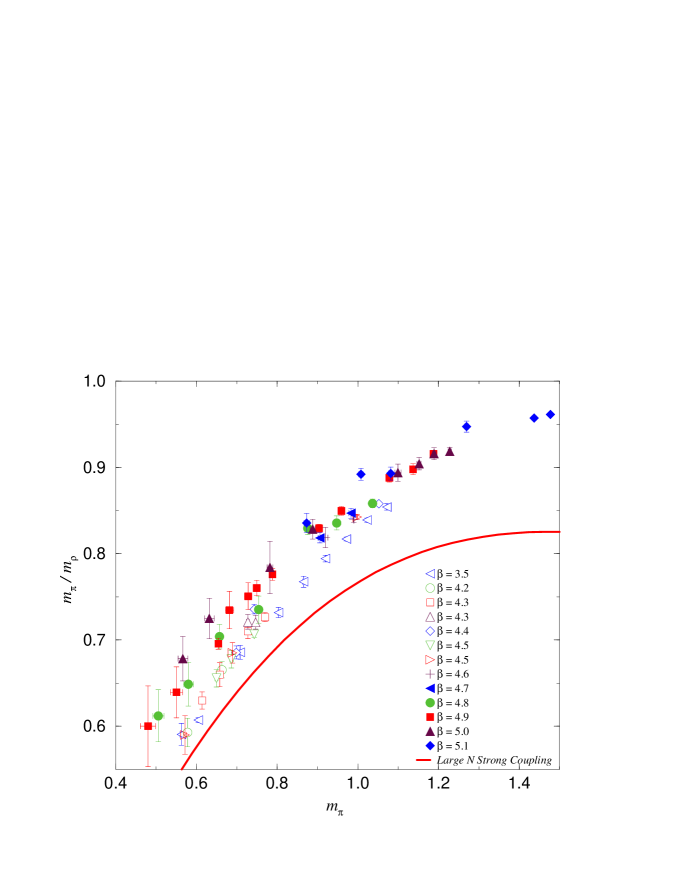
Our first result is the unmatchability of the data at . We find that must be larger than . Figure 1 shows the two points obtained at on the larger lattice (with appropriately scaled by a factor of 2) and the corresponding data for and on the smaller volume for . Data points obtained at larger values lie to the left of those from (see figure 5).
3.2 Matching at
Our second result is that at matching is possible. Figure 2 shows the matching with on the smaller lattice. It is interesting to note that all three points, at different values of , match with corresponding points at the same value of . For comparison similar points obtained at and on the smaller lattice are shown. For tends to be lower than the values at , whereas at they are higher. Two conclusions follow from this data: the first is that the data at is consistent with a value of , and second that this matching is the same for all three different values of used, indicating a independence of the -function.
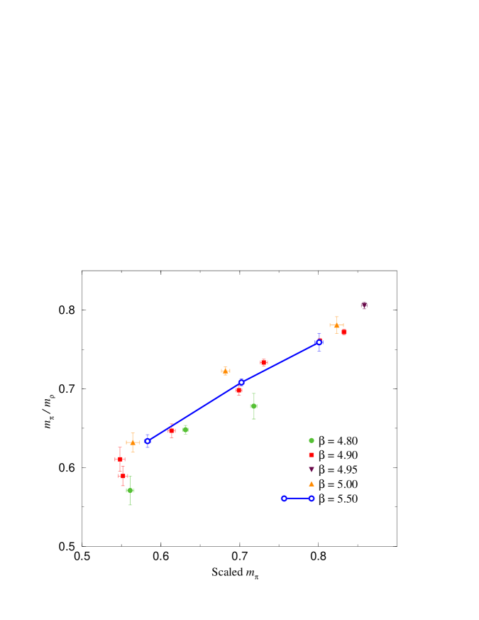
At the central matching value () we find , , and for large lattice values , , and respectively, thus giving an estimate of the integrated -function.
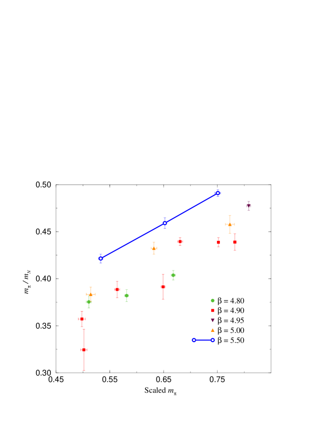
On the other hand, figure 3 shows that the the system is not in the scaling region because the pion-nucleon mass ratio does not match for the same values of and .
Another set of observables which we can match to determine are appropriate ratios of Wilson loops, just as was done for pure gauge theories [8]. We computed space-like planar Wilson loops on all our lattice configurations and evaluated ratios of two or four Wilson loops arranged such that the corner and perimeter singularities cancel between numerator and denominator,
We then determined from the condition
on the smaller lattice was tuned such that the mass on the smaller lattice was twice that on the larger lattice. In practice we interpolated (or extrapolated) linearly from two simulations on the smaller lattice with slightly different values of . Unfortunately, with our statistics the errors on the larger Wilson loops grew quickly and they were not useful for the ratio matching. With smaller Wilson loops dominating the ratios lattice artefacts in the matching become important. We tried to avoid this by considering tree level and one-loop improved ratios [8]. For the matching of the data, for example, depending on various “cuts” imposed on the ratios considered, such as the minimum perimeter and area of the Wilson loops and the maximum relative error, we obtained average values between and . This is somewhat smaller than the preferred value from the matching of , indicating again that we are not yet in the regime of a unique, observable independent -function.
The static quark potential provides us with another matching condition between the large and small lattices. We computed finite approximations to the static quark potential using time-like Wilson loops which were constructed using “APE”-smeared spatial links [9, 6]. On- and off-axis spatial paths were used with distances , , , and , with a positive integer. The “effective” potentials
were fitted using a correlated procedure with the spatial covariance estimated using the bootstrap method. The potential on the large lattice was fitted to the form222We note that we never observed string breaking.
the last term takes account of the lattice artifacts at short distance. Here, denotes the lattice Coulomb potential for the Wilson gluonic propagator.
In figure 4, we plot the potential for the lattice with and scaled to a spatial lattice of length . Also plotted are the potentials for the lattices with and , and and : the latter point only has the on-axis values shown. These points have nearly matching pion-rho ratios.
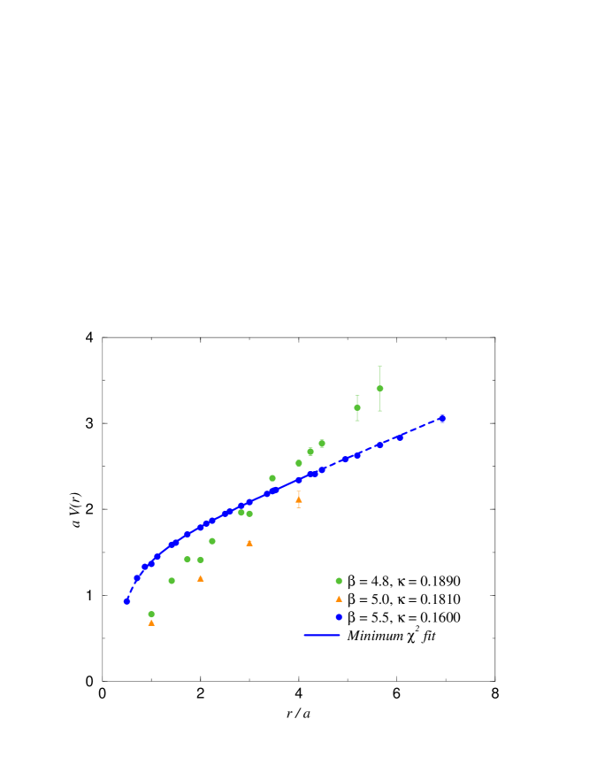
We can see that the potentials do not match the lattice. While we do not expect the constant to match between the fine and coarse lattices, it is clear that the slopes of the coarse lattice potentials are too large. The slope decreases with increasing , indicating that the shift required for matching the potential is smaller than that required for matching and closer to that of the Wilson loops ratios. We also see large violations of rotational symmetry in the coarse lattice potential compared to the finer lattice potential, indicating that the coarse lattice is at relatively strong coupling.
3.3 Parameter reduction at strong coupling
A third result is an approximate parameter reduction in the theory at strong coupling ( to ). Figure 5 includes all our data in this range of on the smaller lattice and shows that for the data is essentially a function of only a single parameter. Any change in may be compensated for by a change in . This is consistent with the large strong coupling result of Kawamoto and Smit [10], which for and gives
4 Conclusions
Combining the present results with those obtained earlier on smaller lattices [3] we find the -function shown in figure 6. It is similar to that found for pure lattice gauge theory with the Wilson gauge action. We are led to the conclusion that current dynamical simulations are being done at strong coupling.
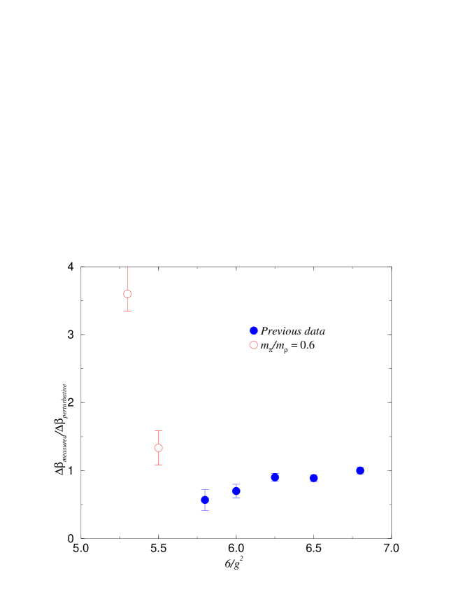
Indeed, not only do we find that for the -function does not agree with the perturbative predictions (asymptotic scaling), but that different renormalization conditions give different estimates for the -function: the shift which gives satisfactory matching for and fails to match , ratios of Wilson loops, or the potential. In other words we do not even observe a universal but non-perturbative -function (scaling).
One therefore may need to reassess estimates for parameters and hence the cost of future computations with dynamical Wilson fermions accordingly.
Acknowledgements
This research was supported by by the U.S. Department of Energy through Contract Nos. DE-FG05-92ER40742 and DE-FC05-85ER250000.
References
- [1] K. Akemi, M. Fujisaki, M. Okuda, Y. Tago, P. de Forcrand, T. Hashimoto, S. Hioki, O. Miyamura, T. Takaishi, A. Nakamura, and I. O. Stamatescu. Scaling study of pure gauge lattice QCD by Monte Carlo renormalization group method. Phys. Rev. Lett., 71:3063–3066, 1993.
- [2] T. Blum, Leo Karkkainen, D. Toussaint, and Steven Gottlieb. The function and equation of state for QCD with two flavors of quarks. Phys. Rev., D51:5153–5164, 1995.
- [3] K. M. Bitar, A. D. Kennedy, and P. Rossi. The QCD -function with dynamical Wilson fermions. In Andreas S. Kronfeld and Paul B. Mackenzie, editors, Lattice ’88, volume B9 of Nuclear Physics (Proceedings Supplements), pages 469–472, 1989. Proceedings of the 1988 Symposium on Lattice Field Theory, Fermilab.
- [4] Khalil M. Bitar, A. D. Kennedy, and Pietro Rossi. The QCD -function with dynamical Wilson fermions. Phys. Rev. Lett., 63:2713, 1989.
- [5] Khalil M. Bitar, Thomas A. DeGrand, Robert G. Edwards, S. A. Gottlieb, Urs M. Heller, A. D. Kennedy, John B. Kogut, A. Krasnitz, Weiqiang Liu, Michael C. Ogilvie, R. L. Renken, Pietro Rossi, D. K. Sinclair, R. L. Sugar, D. Toussaint, and K. C. Wang. Hadron spectrum and matrix elements in QCD with dynamical Wilson fermions at . Phys. Rev., D49(7):3546–3562, April 1994.
- [6] Khalil M. Bitar, Robert G. Edwards, Urs M. Heller, and A. D. Kennedy. Preprint, SCRI, 1996. In preparation.
- [7] Khalil M. Bitar, Robert G. Edwards, Urs M. Heller, A. D. Kennedy, and Pavlos Vranas. Towards the QCD function with dynamical Wilson fermions. In Frithjof Karsch, Jurgen Engels, Edwin Laermann, and Bengt Petersson, editors, Lattice ’94, volume B42 of Nuclear Physics (Proceedings Supplements), pages 796–798, 1995. Proceedings of the International Symposium on Lattice Field Theory, Bielefeld, Germany, 27 September–1 October 1994.
- [8] Anna Hasenfratz, Peter Hasenfratz, Urs Heller, and Frithjof Karsch. The function of the SU(3) Wilson action. Phys. Lett., 143B:193, 1984.
- [9] M. Albanese and al. Glueball masses and string tension in lattice QCD. Phys. Lett., 192B:163, 1987. (APE collaboration).
- [10] N. Kawamoto and J. Smit. Effective Lagrangian and dynamical symmetry breaking in strongly coupled lattice QCD. Nucl. Phys., B192:100, 1981.