Anti-Ferromagnetic Condensate in Yang-Mills Theory

Abstract

SU(2) gauge theory with competing interactions is shown to possess a rich phase structure with anti-ferromagnetic vacua. It is argued that the phase boundaries persist in the weak coupling limit suggesting the existence of different renormalized continuum theories for QCD.

and

1 Introduction

Non-renormalizable models are traditionally ignored in high energy physics due to their lack of predictive power. In fact, one needs infinitely many counter terms and renormalization conditions to render these theories well defined. In the framework of the renormalization group [1] one usually identifies the ultraviolet fixed point, where the correlation length diverges with the renormalized theory [2]. In the vicinity of the fixed point the renormalization group equations can be linearized. The resulting scaling law allows to define relevant, marginal or irrelevant operators. These are the eigen-operators of the linearized renormalization group equation with increasing, constant or decreasing coefficients as the cut-off is lowered. It is of central importance that the class of relevant and marginal operators is equivalent to the class of renormalizable operators. This can be seen from a comparison of two renormalized trajectories, one with relevant or marginal couplings, the other one with additional contributions from irrelevant operators. The trajectories approach each other at the infrared end of the region of linearizability. The difference between the two theories reduces to an overall scale factor only as the cut-off is moved towards the infrared. This shows that the presence of irrelevant operators prevents the trajectory to approach the fixed point as the cut-off is removed. In fact, if the irrelevant coupling constant decreases in the infrared direction, then it increases as the cut-off is enlarged.

Universality in the sense of independence on microscopical details of the system implies that effects of irrelevant coupling constants die out at physical scales. However, indications of continuum physics beyond the class of traditionally renormalizable theories do exist. One example to enlarge the class of theories, which characterize the physics of a given particle and symmetry pattern, is based on the presence of multiple fixed points [3]. Another, more conventional possibility exists, when strong anomalous dimensions arise from non-perturbative effects. These effects have been shown to change the sign of critical exponents from negative to positive values [4, 5]. For $RP^{N-1}$ models, the role of non-perturbative topological defect structures, which may survive the weak coupling limit and influence the universality class of the theory, is under vigorous discussion [6, 7, 8, 9].

In this paper we present indications that the non-perturbative generation of additional relevant operators leading to competing interactions might also be present in non-Abelian gauge theories. Competing interactions are also relevant for Yukawa models, where the existence of nontrivial fixed points and the crossover between universality classes has been investigated [10].

We begin with a brief review of the basic mechanism, the effect of higher order derivative terms, which are able to generate competing interactions on the semi-classical vacuum. In section 3 we discuss the possible phases of the gauge models with higher derivatives in the semi-classical picture. The Quantum Field Theoretical aspects of the anti-ferromagnetic phase are briefly commented in Section 4. Our lattice gauge model is introduced in section 5. In the following chapter we present numerical results and discuss the phase structure. The vital issue of the continuum limit is addressed in section 7. Finally we give a summary and conclude with some speculative remarks.

2 Non-Perturbative Effects at the Cut-off

The renormalization group functions, which determine the effective coupling constants are usually computed perturbatively. There are some non-asymptotically free models, where strong interactions at the cut-off modify the evolution of the coupling constants in a manner, which influences the long range structure of the vacuum. The formation of small positronium bound states in strong coupling massless QED [4] is an example, where a strong anomalous dimension generates new relevant operators [5]. Furthermore, the two dimensional Sine-Gordon model has a phase transition at strong coupling, where the normal ordering is not sufficient to remove the ultraviolet singularities [11]. Another description of this phase transition can be derived from the equivalence of the Sine-Gordon and the X-Y model. It turns out that the strong coupling phase of the Sine-Gordon theory is dual to the ionized vortex phase of the X-Y model [12]. In this phase the vortex fugacity becomes a new relevant coupling constant.

We want to address the question of condensate formation at the cut-off scale in non-Abelian gauge models. For simplicity we consider an SU(2) gauge model with additional higher derivative terms in the action. It is defined by the Lagrangian

$${{\cal L}}=-{1\over 4g^{2}}~{}F^{a}_{\mu\nu}\biggl{(}\delta^{ab}+{c_{2}\over\Lambda^{2}}{\cal D}^{2ab}+{c_{4}\over\Lambda^{4}}{\cal D}^{4ab}\biggr{)}F^{b\mu\nu}~{}~{},$$ (1)

where ${\cal D}^{ab}_{\mu}$ is the covariant derivative. There are two different ways of looking at this modified theory. One possibility is to start with a theory of elementary particles. In this case the cut-off has to be removed and the $\Lambda$-parameter must be identical to the cut-off in order to eliminate overall UV divergences. The new terms in the action can be regarded as a variant of the Pauli-Villars regulator. The theory is renormalizable in the framework of a perturbative expansion in $g^{2}$ and $c_{\alpha}$ around the configuration with $A_{\mu}(x)=0$ [13, 14], provided the one-loop level is regulated [15]. Another possibility is to consider a unified model, where a heavy particle is coupled to a Yang-Mills field. The elimination of the heavy particle generates new terms in the Lagrangian of eq.1. Consider a sequence of theories in particle physics, ${\cal T}_{k}$ with characteristic energy scales $\Lambda_{k}$, $\Lambda_{k+1}>\Lambda_{k}$ ($k=0,1,\cdots,N$), where ${\cal T}_{N}$ is the Theory of Everything (TOE) and ${\cal T}_{k}$ is an effective theory of ${\cal T}_{k+1}$ with cut-off ${\cal O}(\Lambda_{k+1})$. The particle exchange at the characteristic scale of ${\cal T}_{k+1}$ generates relevant and irrelevant operators for ${\cal T}_{k}$ according to the decoupling theorem [16]. Though irrelevant couplings are suppressed as ${\cal O}(\Lambda_{k}^{2}/\Lambda_{k+1}^{2})$, they are important because they represent physics beyond the scale $\Lambda_{k}$. In their absence high energy scaling would be described by ${\cal T}_{k}$ and the renormalized trajectory would end at the UV fixed point of ${\cal T}_{k}$. These irrelevant coupling constants are the physical regulators of ${\cal T}_{k}$. In this case no attempt is made to remove the cut-off of this effective theory.

An observable $A$ at momentum scale $\mu$ has a perturbative expansion:

$$A=\mu^{[A]}\sum_{klm}I_{klm}~{}g^{k}\biggl{(}c_{2}{\mu^{2}\over\Lambda^{2}}\biggr{)}^{l}~{}\biggl{(}c_{4}{\mu_{4}\over\Lambda^{4}}\biggr{)}^{m}~{}~{},$$ (2)

where $I_{klm}$  is a dimensionless loop integral. In the absence of infrared singularities observables are independent of $c_{2}$ and $c_{4}$ far away from the cut-off. This demonstrates the irrelevance of coupling constants with negative mass dimension. The important question now is, whether this argument, which is based on an expansion around the trivial vacuum, $A_{\mu}=0$, remains valid in the presence of an inhomogeneous condensate.

To answer this question, first consider the action corresponding to an instanton with scale parameter $\rho$ [17]

$$S_{inst}(\rho)={8\pi^{2}\over g^{2}}~{}\biggl{(}1-{\tilde{c}_{2}\over(\rho\Lambda)^{2}}+{\tilde{c}_{4}\over(\rho\Lambda)^{4}}\biggr{)}~{}~{},$$ (3)

where $\tilde{c}_{\alpha}=O(c_{\alpha})>0$. This action agrees with the renormalized value, $8\pi^{2}/g^{2}$, for large instantons. As the instanton size approaches the length scale $\Lambda^{-1}$ we find deviations from scale invariance and a minimum is reached in the vicinity of the cut-off,

$$S_{0}=S(\rho_{0})={8\pi^{2}\over g^{2}}\biggr{(}1-{\tilde{c}_{2}^{2}\over 4\tilde{c}_{4}}\biggr{)}~{}~{},$$ (4)

where

$$\rho_{0}=\Lambda^{-1}\sqrt{{2\tilde{c}_{4}\over\tilde{c}_{2}}}~{}~{}~{}~{}.$$ (5)

Since the mini-instanton action is not a simple polynomial of the coupling constants it generates a combination of $c_{2}$ and $c_{4}$, which is independent of the subtraction scale $\mu$ and the result depends on $c_{\alpha}$ in contrast to eq.2. The absence of the usual power suppression in the infrared region opens the possibility of an eventual modification of the universality class.

In order to find a regime of the coupling constants, where the mini-instantons dominate we increase $c_{2}$. At some critical value $c_{0}$ of $c_{2}$ the mini-instanton gas will dominate the path integral. Beyond this point $c_{2}>c_{0}$ we find negative values of the action given by eq.4. This is a radically new territory. The negative instanton action imposes frustration on the vacuum. It becomes energetically favorable to fill the vacuum with instantons. The resulting semi-classical ground state will be a crystal of instantons. For small $g^{2}$ the instanton lattice is densely packed and lattice vibrations are strongly suppressed. The translation and rotation invariance of this semi-classical vacuum will be broken just as in the case of an ionic lattice in solid state physics. As long as CP symmetry is preserved the total winding number of the vacuum vanishes. Then the crystal consists of alternating instantons and anti-instantons similar to an anti-ferromagnetic (AF) Néel state.

The matching between the topology of internal and external spaces is not essential in establishing the AF order, in contrast with discrete spin models. In fact, the eigenvalue of small fluctuations around $A_{\mu}=0$ with momentum $p$ in Feynman gauge is given by

$$\lambda(p^{2})=p^{2}\biggl{(}1-c_{2}{p^{2}\over\Lambda^{2}}+c_{4}{p^{4}\over\Lambda^{4}}\biggr{)}~{}~{}.$$ (6)

The instability, $\lambda(p^{2})<0$, occurs for momenta

$${1\over 2}-\sqrt{{c_{2}^{2}-4c_{4}\over 4c_{4}^{2}}}<{p^{2}\over\Lambda^{2}}<{1\over 2}+\sqrt{{c_{2}^{2}-4c_{4}\over 4c_{4}^{2}}}~{}~{}~{}~{}.$$ (7)

When $c_{2}>2\sqrt{c_{4}}$ this leads to a condensation of particles in this momentum range until their repulsive interactions stabilize the vacuum. The result will be a condensate with staggered order parameter in the middle of the Brillouin-zone, $p\approx\Lambda/2$.

3 Phase Structure

One expects three qualitatively different phases shown in fig.1 for a continuum theory with the Lagrangian of eq.1:

Figure 1: Size dependence of the instanton action in the three different phases of the gauge theory. Full and long dashed lines correspond to $c_{\alpha}=0$ and $c_{2}<0$, respectively, and belong to phase 1. The short dashed line stands for $c_{2}>c_{0}$, $c_{4}>0$, which corresponds to phase 2. The AF phase 3 is shown by a dotted line.

1. Classically scale invariant phase: $c_{\alpha}=0$. The theory should be in the same universality class as the one with $c_{2}<0$ and $c_{4}>0$. For this choice of the new coupling constants, $c_{\alpha}$, the saddle points, i.e. $A_{\mu}=0$ and instantons with cut-off independent size parameter are not influenced by $c_{\alpha}$ and remain in the infrared. As a consequence the usual argument for the irrelevance as explained in context of eq.2 applies. This is the usual phase of the Yang-Mills system known from dimensional regularization.

2. Mini-instanton phase: $c_{4}>0$, $c_{0}>{c^{2}_{2}\over c_{4}}>0$ and $S_{0}$ is small and positive. The path integral is dominated by instantons with size close to the cut-off. The saddle points in the ultraviolet regime generate different beta-functions and the physics changes discontinuously between phases one and two.

3. Anti-ferromagnetic phase: ${c^{2}_{2}\over c_{4}}>c_{0}$ so that $S_{0}<0$. The semi-classical vacuum is an instanton lattice with alternating topological charge. One finds this reminiscent of the Néel state of solid state physics at $p\approx\Lambda/2$. Further splitting into sub-phases without anti-ferromagnetic long range order is possible. Renormalizability is a highly non-trivial issue.

The usual attitude towards mini-instantons, alias topological defects [18], is to suppress them either by improving the action [19], or the definition of the winding number [20], in order to stay in phase one. The attempt to eliminate these modes originates from the naive semi-classical picture, where the configurations that dominate the path integral are solutions of the renormalized, cut-off independent equations of motion. But this is not necessarily so [21]. The d-dimensional lattice regulated path integral is saturated by configurations, whose variation from site-to-site is

$$\Delta\phi(x)=O(a^{1-{d\over 2}})~{}~{}~{}~{}.$$ (8)

This result is the real space equivalent to the momentum space power counting rule. For a free massless theory it can be derived from the path integral

$$\prod_{x}\int d\phi(x)~{}~{}\mbox{e}^{-{1\over 2}a^{d-2}\sum_{x,\mu}(\phi(x+\mu)-\phi(x))^{2}}~{}~{}~{}~{}.$$ (9)

The Gaussian integration yields eq.8, which leads to continuous but nowhere differentiable trajectories in quantum mechanics for $d=1$ [22], finite, cut-off independent discontinuities and non-trivial phase structure for $d=2$ [12], and Dirac delta singularities in higher dimensions [23]. It is a complicated dynamical issue, whether smoothness prevails for certain observables in quantum field theory.

Recent improvements [24], go so far as to try to cancel all power corrections to the scale invariant action. This certainly brings the improved lattice theory close to the renormalized trajectory of perturbative QCD known from dimensional regularization. Our strategy is just the opposite. We exploit the richness of gauge theories by varying the dynamics close to the cut-off and see, whether non-perturbative effects generate new quantum field theories.

It has been known that competing interactions create rich phase structure. An AF phase is found, where frustrations stabilized by the balance of repulsive and attractive forces form a densely packed lattice. Systems showing frustration have first been investigated in the framework of solid state physics [31], where it was found that the AF phase usually consists of several layered sub-phases. Recent results obtained for the four dimensional Ising model [32, 33], the three dimensional $Z_{3}$ [34] Potts model with ferromagnetic (FM) nearest neighbour (NN) and AF next to nearest neighbour (NNN) couplings can be considered as generic. Starting in the FM phase and increasing the strength of the AF coupling we enter a phase with AF order in one or two directions. Further increase of the AF coupling induces more directions to show AF behaviour. Completely AF order may or may not be reached for strong AF coupling depending on the matching of space-time and the internal dimensions. The AF phase has already been considered in ref. [35] where perturbative arguments for the existence of a non-trivial UV limit of the lattice $\phi^{4}$ theory were found.

4 Anti-Ferromagnetic Vacuum

The use of AF condensates in Quantum Field Theories deserves special attention due to additional difficulties with reflection positivity and the construction of the continuum limit. When eq.1 is considered as an effective theory obtained from the perturbative elimination of a particle with mass $M={\cal O}(\Lambda)$, the cut-off, $\Lambda$, is kept finite. This model has two phases, the usual one with $S_{0}>0$ and a frustrated phase where $S_{0}<0$. The length scale of the frustrated vacuum, i.e. the lattice spacing of the instanton-anti instanton crystal, ${\cal O}(\Lambda^{-1})$, is kept finite. It is difficult to describe the physics beyond the energy $\Lambda$, the heavy particle threshold, by an effective theory without the heavy particle as a dynamical degree of freedom. In this energy regime the propagating heavy particle and its open channels make the truncation of the effective action in eq.1 to ${\cal O}(\Lambda^{-4})$ a very poor approximation. To point out a systematic approach to this problem we remark that the time evolution is unitary in a positive definite Hilbert space for a well defined Quantum Field Theory. In the Euclidean domain this translates to reflection positivity [36]. A sufficient condition for reflection positivity of the single plaquette action $S=\sum_{j}c_{j}\sum_{x,\mu\nu}\mbox{Tr}_{j}(1-U_{\mu\nu}(x))$ where $\mbox{Tr}_{j}$ denotes the trace in a representation labeled by $j$ is that the coefficients of the traces are positive for each representation. The lattice regulated version of eq.1 contains negative coefficients in front of the traces in the Lagrangian and the issue of the reflection positivity is unclear.

We believe that the problem with unitarity has a deeper origin. In a renormalization procedure a blocking step unavoidably generates coupling constants with negative sign. These couplings represent interactions between remote sites on the lattice. Does this mean that the concept of unitarity or reflection positivity is not renormalization group invariant ? This might be so because even the transfer matrix formalism is lost after a blocking step due to the presence of higher order derivatives in the action. When degrees of freedom are eliminated in a quantum system pure states become mixed states and one should use the density matrix formalism. Higher order derivative terms responsible for the loss of the transfer matrix formalism represent correlations which are usually taken into account by the density matrix formalism. As long as they are irrelevant this mixing of different quantum states is negligible. In fact, in the ultraviolet scaling regime of the trivial or ferromagnetic vacuum where higher order derivatives are certainly irrelevant the effects of heavy modes eliminated by the blocking step are local and a violation of unitarity is observable only at short distances.

This lets us speculate that a generalization of unitarity or reflection positivity to AF systems is possible by relaxing these conditions in the ultraviolet region and demanding their strict validity only at physical length scales, i.e. in the continuum limit.

It has been long known that higher order derivatives can generate new degrees of freedom with negative norm which violate unitarity [37]. The violation of unitarity can be understood looking at the frequency integration in perturbative loop integrals. Higher powers of the momentum in the denominator lead to poles at complex frequencies giving non-unitary contributions. The usual strategy to recover unitarity is to fine tune the parameters of the theory so that the poles appear in complex conjugate pairs and the imaginary part of their contribution cancel [38, 39]. No violation of unitarity is detected at finite energy in the perturbative solution when the scale of the coupling constants of higher order derivatives, $\Lambda$, approaches infinity. Such a solution seems to support our suggestion above, namely to relax the strict conditions imposed at all scales. However, the vacuum considered in this paper is non-homogeneous and the argument of ref. [38, 39] is not sufficient to exclude the violation of unitarity.

We think that the problem with unitarity and reflection positivity can be solved for the AF vacuum. The AF phase has actually been observed in Solid State Physics for quantum systems. How does the anti-ferromagnetic Heisenberg model retain reflection positivity despite the negative sign of its coupling constant? An illuminating example is worked out in ref. [40] where the quantum mechanics of a $Z_{4}$ variable is considered. It is found that the transfer matrix, $T$, may have real but negative eigenvalues when the coupling is ”anti-ferromagnetic” in time. It is suggested to impose reflection positivity for the square of the transfer matrix, $T^{2}$, only. Note that $T^{2}$ describes the jump in time by the period length of the ”anti-ferromagnetic” vacuum in time. This agrees with our intuition: The AF vacuum reflects the presence of periodic structures in space or time. There should be no problem with unitarity if

• the vacuum is static, ”ferromagnetic”, or

• only those powers of the transfer matrix are taken into account whose time step is an integer multiple of the period length.

As a slight generalization of this conjecture we expect that the renormalized trajectory arising from a blocking procedure which preserves the AF order, [41], maintains reflection positivity.

The construction of the continuum limit, $\Lambda\to\infty$, of eq.1 raises the question of renormalizability. Although not required for realistic, i.e. effective theories, it simplifies ultraviolet scaling laws and eliminates the unphysical complications at high energies in the anti-ferromagnetic vacuum. However, in Quantum Field Theories with AF vacuum renormalizability has another important role. The inhomogeneous vacuum violates conservation laws related to external symmetries. The space-time symmetries of the continuum Quantum Field Theory are recovered as the length scales of both the anti-ferromagnetic condensate and the cutoff vanish.

The renormalized theory is defined at the critical point, where at least one of the correlation lengths of different particle sectors diverges. The selection of one sector with diverging correlation length and keeping the corresponding particle mass constant fixes the value of the cutoff. Other sectors, where the correlation length diverges slower or faster when the critical point is approached correspond to infinitely heavy or massless excitations, respectively. The physical content of the theory in this limit can depend on the direction in which the critical point is approached.

The continuum limit of an AF vacuum is a rather involved problem. Analytical methods based on an expansion around homogeneous or slowly varying field configurations are inadequate for its study. In fact, in the presence of an AF condensate the plaquettes differ from a constant configuration by a finite amount, so that $<A_{\mu}>=\Lambda O(g^{-1})$. Such an extremely strong field can modify the UV scaling laws verified rigorously in ref. [42].

The particle content of a theory can be studied by the help of Bloch-waves. The excitations above a vacuum which has $N_{0}$ degrees of freedom in an elementary cell give rise to $N_{0}$ dispersion relations, the bands in the language of Solid State Physics. There might be several particles corresponding to a single quantum field. Some of the bands may correspond to excitations whose mass diverges with the cut-off. These heavy particles decouple from the physics during the renormalization procedure. The others are renormalized and describe particle-like excitations with finite mass.

The renormalized AF vacuum possesses a condensate whose characteristic length approaches zero and becomes unresolvable for observables which are defined at finite scales. As a consequence, both the AF and the ferromagnetic vacuum appear homogeneous after renormalization. What distinguishes these phases are the excitations above the vacuum. The ultraviolet fixed point was studied in ref. [43] when only one particle mass was kept finite during the renormalization. The situation is similar to lattice fermions which form an anti-ferromagnetic vacuum [44]. If some of the particle modes acquire a mass proportional to the cut-off a generalization of the decoupling theorem, [16, 43], to anti-ferromagnetic vacua can be used to describe their effects on the particles remaining after renormalization. The renormalization can be studied in a perturbative expansion even when the mass of several particles is kept finite [45].

One expects new universality classes in the AF phase because the interactions between different particle modes of the same field operator are described by vertices which are delocalized within the elementary cell of the vacuum. A study of the two dimensional Ising model revealed new critical points and relevant operators in the AF phase compared to the disordered and ferromagnetic phases [41]. The negative eigenvalue of the transfer matrix mentioned above introduces a staggered mode at arbitrary distance. This gives an example how the ultraviolet structure of the vacuum may modify long range correlations.

5 Lattice Regulated Model

The lattice regulated version of the irrelevant operator $F^{a}_{\mu\nu}{\cal D}^{2n\/ab}F^{b\mu\nu}$ corresponds to a linear superposition of Wilson loops up to size $2n\times 2n$. Although it is straightforward to find a lattice version of the action defined in eq.1, we choose an even simpler, more local form of the lattice action. In fact, we do not have to rely on the tree level stability of instantons in a fully non-perturbative numerical computation. It is sufficient to use a modified action, which includes negative contributions from short scale fluctuations [35]. This can be achieved with an extended lattice action, which contains planar $1\times 1$, $1\times 2$ and $2\times 2$ loops,

$$S= c_{1} S_{1x1}+c_{2}S_{1x2}+c_{3}S_{2x2}$$

$$= c_{1} \sum_{x,\mu>\nu}{\mbox{Tr~{}}}\left(1-\raisebox{-5.69046pt}{ \begin{picture}(1.2,1.2)(-0.6,-0.6) \put(-0.5,-0.5){\line(1,0){1.0}} \put(0.5,-0.5){\line(0,1){1.0}} \put(0.5,0.5){\line(-1,0){1.0}} \put(-0.5,0.5){\line(0,-1){1.0}} \put(0.0,-0.5){\vector(1,0){0.0}} \put(0.5,0.0){\vector(0,1){0.0}} \put(0.0,0.5){\vector(-1,0){0.0}} \put(-0.5,0.0){\vector(0,-1){0.0}} \put(-0.5,-0.5){\circle*{0.2}} \put(-0.55,-0.55){\makebox(0.0,0.0)[tr]{\footnotesize$x$}} \put(-0.55,0.0){\makebox(0.0,0.0)[r]{\footnotesize$\nu$}} \put(0.0,-0.55){\makebox(0.0,0.0)[t]{\footnotesize$\mu$}} \end{picture}}\right)$$

$$+ c_{2} \sum_{x,\mu>\nu}\left[~{}{\mbox{Tr~{}}}\left(1-\raisebox{-5.69046pt}{ \begin{picture}(2.2,1.2)(-1.1,-0.6)\put(-1.0,-0.5){\line(1,0){2.0}} \put(-1.0,0.5){\line(1,0){2.0}} \put(-1.0,-0.5){\line(0,1){1.0}} \put(1.0,-0.5){\line(0,1){1.0}} \put(-0.5,-0.5){\vector(1,0){0.0}} \put(0.5,-0.5){\vector(1,0){0.0}} \put(-0.5,0.5){\vector(-1,0){0.0}} \put(0.5,0.5){\vector(-1,0){0.0}} \put(-1.0,0.0){\vector(0,-1){0.0}} \put(1.0,0.0){\vector(0,1){0.0}} \put(-1.0,-0.5){\circle*{0.2}}\put(0.0,-0.5){\circle*{0.2}}\put(1.0,-0.5){\circle*{0.2}} \put(-1.0,0.5){\circle*{0.2}}\put(0.0,0.5){\circle*{0.2}}\put(1.0,0.5){\circle*{0.2}} \put(-1.0,-0.55){\makebox(0.0,0.0)[tr]{\footnotesize$x$}} \put(-1.0,0.0){\makebox(0.0,0.0)[r]{\footnotesize$\nu$}} \put(0.0,-0.55){\makebox(0.0,0.0)[t]{\footnotesize$\mu$}} \end{picture}}\right)+{\mbox{Tr~{}}}\left(1-\raisebox{-14.22636pt}{ \begin{picture}(1.2,1.2)(-0.6,-0.6)\put(0.25,-0.5){\line(0,1){1.0}} \put(0.25,0.5){\line(-1,0){0.5}} \put(-0.25,0.5){\line(0,-1){1.0}} \put(0.2,0.0){\line(1,0){0.05}} \put(-0.25,-0.5){\circle*{0.1}} \put(-0.25,0.5){\circle*{0.1}} \put(0.25,-0.5){\circle*{0.1}} \put(0.25,0.5){\circle*{0.1}} \put(-0.25,0.0){\circle*{0.1}} \put(0.25,0.0){\circle*{0.1}} \put(-0.25,-0.35){\vector(0,-1){0.0}} \put(-0.25,0.15){\vector(0,-1){0.0}} \put(-0.1,0.5){\vector(-1,0){0.0}} \put(0.25,0.35){\vector(0,1){0.0}} \put(0.25,-0.15){\vector(0,1){0.0}} \put(-0.25,-0.5){\line(1,0){0.5}} \put(0.1,-0.5){\vector(1,0){0.0}} \put(-0.3,-0.55){\makebox(0.0,0.0)[tr]{\footnotesize$x$}} \put(-0.3,0.0){\makebox(0.0,0.0)[r]{\footnotesize$\nu$}} \put(0.0,0.8){\makebox(0.0,0.0)[t]{\footnotesize$\mu$}} \end{picture}}\right)\right]$$

$$+ c_{3} \sum_{x,\mu>\nu}{\mbox{Tr~{}}}\left(1-\raisebox{-14.22636pt}{ \begin{picture}(1.2,1.2)(-0.6,-0.6) \put(-0.5,-0.5){\line(1,0){1.0}} \put(0.5,-0.5){\line(0,1){1.0}} \put(0.5,0.5){\line(-1,0){1.0}} \put(-0.5,0.5){\line(0,-1){1.0}} \put(-0.5,-0.5){\circle*{0.1}} \put(-0.5,0.5){\circle*{0.1}} \put(0.5,-0.5){\circle*{0.1}} \put(0.5,0.5){\circle*{0.1}} \put(0.0,-0.5){\circle*{0.1}} \put(0.0,0.5){\circle*{0.1}} \put(0.5,0.0){\circle*{0.1}} \put(-0.5,0.0){\circle*{0.1}} \put(-0.25,-0.5){\vector(1,0){0.0}} \put(0.25,-0.5){\vector(1,0){0.0}} \put(0.5,-0.25){\vector(0,1){0.0}} \put(0.5,0.25){\vector(0,1){0.0}} \put(-0.25,0.5){\vector(-1,0){0.0}} \put(0.25,0.5){\vector(-1,0){0.0}} \put(-0.5,-0.25){\vector(0,-1){0.0}} \put(-0.5,0.25){\vector(0,-1){0.0}} \put(-0.55,-0.55){\makebox(0.0,0.0)[tr]{\footnotesize$x$}} \put(-0.55,0.0){\makebox(0.0,0.0)[r]{\footnotesize$\nu$}} \put(0.0,-0.55){\makebox(0.0,0.0)[t]{\footnotesize$\mu$}} \end{picture}}\right)\quad,$$ (10)

where our notation follows the definitions of ref. [25]. For completeness, we present the dependence of the action on a specific link. The action per link $U_{\mu}(x)$, which is needed in the heat-bath algorithm, is given by

$$S(U_{\mu}(x))=2~{}{\mbox{Re~{}}}{\mbox{Tr~{}}}[1-U_{\mu}(x)\tilde{U}_{\mu}(x)]\quad.$$ (11)

It contains the sum of the staples associated with the Wilson loops appearing in the extended action, eq.10,

$$\tilde{U}_{\mu}(x)=\sum_{{\nu}\atop{\nu\neq\mu}} c_{1} \left(~{}\raisebox{-5.69046pt}{ \begin{picture}(1.2,1.2)(-0.6,-0.6)\put(0.5,-0.5){\line(0,1){1.0}} \put(0.5,0.5){\line(-1,0){1.0}} \put(-0.5,0.5){\line(0,-1){1.0}} \put(0.5,0.0){\vector(0,-1){0.0}} \put(0.0,0.5){\vector(1,0){0.0}} \put(-0.5,0.0){\vector(0,1){0.0}} \put(-0.5,-0.5){\circle*{0.2}} \put(-0.55,-0.55){\makebox(0.0,0.0)[tr]{\footnotesize$x$}} \put(-0.55,0.0){\makebox(0.0,0.0)[r]{\footnotesize$\nu$}} \put(0.0,0.55){\makebox(0.0,0.0)[b]{\footnotesize$\mu$}} \end{picture}}+\raisebox{-5.69046pt}{ \begin{picture}(1.2,1.2)(-0.6,-0.6)\put(0.5,-0.5){\line(0,1){1.0}} \put(0.5,-0.5){\line(-1,0){1.0}} \put(-0.5,0.5){\line(0,-1){1.0}} \put(0.5,0.0){\vector(0,1){0.0}} \put(0.0,-0.5){\vector(1,0){0.0}} \put(-0.5,0.0){\vector(0,-1){0.0}} \put(-0.5,0.5){\circle*{0.2}} \put(-0.55,0.75){\makebox(0.0,0.0)[tr]{\footnotesize$x$}} \put(-0.55,0.0){\makebox(0.0,0.0)[r]{\footnotesize$\nu$}} \put(0.0,-0.55){\makebox(0.0,0.0)[t]{\footnotesize$\mu$}} \end{picture}}~{}\right)$$

$$+ c_{2} \left(\raisebox{-14.22636pt}{ \begin{picture}(1.2,1.2)(-0.6,-0.6)\put(0.25,-0.5){\line(0,1){1.0}} \put(0.25,0.5){\line(-1,0){0.5}} \put(-0.25,0.5){\line(0,-1){1.0}} \put(-0.25,0.0){\line(1,0){0.1}} \put(-0.1,0.0){\line(1,0){0.1}} \put(0.05,0.0){\line(1,0){0.1}} \put(0.2,0.0){\line(1,0){0.05}} \put(-0.25,-0.5){\circle*{0.1}} \put(-0.25,0.5){\circle*{0.1}} \put(0.25,-0.5){\circle*{0.1}} \put(0.25,0.5){\circle*{0.1}} \put(-0.25,0.0){\circle*{0.1}} \put(0.25,0.0){\circle*{0.1}} \put(-0.25,-0.15){\vector(0,1){0.0}} \put(-0.25,0.35){\vector(0,1){0.0}} \put(0.1,0.5){\vector(1,0){0.0}} \put(0.25,0.15){\vector(0,-1){0.0}} \put(0.25,-0.35){\vector(0,-1){0.0}} \put(-0.3,-0.55){\makebox(0.0,0.0)[tr]{\footnotesize$x$}} \put(-0.3,0.0){\makebox(0.0,0.0)[r]{\footnotesize$\nu$}} \put(0.0,0.8){\makebox(0.0,0.0)[t]{\footnotesize$\mu$}} \end{picture}}+\raisebox{-14.22636pt}{ \begin{picture}(1.2,1.2)(-0.6,-0.6)\put(-0.5,-0.25){\line(0,1){0.5}} \put(-0.5,0.25){\line(1,0){1.0}} \put(0.5,0.25){\line(0,-1){0.5}} \put(0.5,-0.25){\line(-1,0){0.5}} \put(0.0,-0.25){\line(0,1){0.1}} \put(0.0,-0.1){\line(0,1){0.1}} \put(0.0,0.05){\line(0,1){0.1}} \put(0.0,0.2){\line(0,1){0.1}} \put(-0.5,-0.25){\circle*{0.1}} \put(0.0,-0.25){\circle*{0.1}} \put(0.5,-0.25){\circle*{0.1}} \put(-0.5,0.25){\circle*{0.1}} \put(0.0,0.25){\circle*{0.1}} \put(-0.5,0.25){\circle*{0.1}} \put(-0.5,0.1){\vector(0,1){0.0}} \put(-0.15,0.25){\vector(1,0){0.0}} \put(0.35,0.25){\vector(1,0){0.0}} \put(0.5,-0.1){\vector(0,-1){0.0}} \put(0.2,-0.25){\vector(-1,0){0.0}} \put(-0.55,-0.3){\makebox(0.0,0.0)[tr]{\footnotesize$x$}} \put(-0.55,0.0){\makebox(0.0,0.0)[r]{\footnotesize$\nu$}} \put(-0.25,0.5){\makebox(0.0,0.0)[t]{\footnotesize$\mu$}} \end{picture}}+\raisebox{-14.22636pt}{ \begin{picture}(1.2,1.2)(-0.6,-0.6)\put(-0.5,-0.25){\line(0,1){0.5}} \put(-0.5,0.25){\line(1,0){1.0}} \put(0.5,0.25){\line(0,-1){0.5}} \put(0.0,-0.25){\line(-1,0){0.5}} \put(0.0,-0.25){\line(0,1){0.1}} \put(0.0,-0.1){\line(0,1){0.1}} \put(0.0,0.05){\line(0,1){0.1}} \put(0.0,0.2){\line(0,1){0.1}} \put(-0.5,-0.25){\circle*{0.1}} \put(0.0,-0.25){\circle*{0.1}} \put(0.5,-0.25){\circle*{0.1}} \put(-0.5,0.25){\circle*{0.1}} \put(0.0,0.25){\circle*{0.1}} \put(-0.5,0.25){\circle*{0.1}} \put(-0.5,0.1){\vector(0,1){0.0}} \put(0.35,0.25){\vector(1,0){0.0}} \put(-0.15,0.25){\vector(1,0){0.0}} \put(0.5,-0.05){\vector(0,-1){0.0}} \put(-0.35,-0.25){\vector(-1,0){0.0}} \put(0.1,-0.35){\makebox(0.0,0.0)[tr]{\footnotesize$x$}} \put(-0.55,0.0){\makebox(0.0,0.0)[r]{\footnotesize$\nu$}} \put(0.37,0.42){\makebox(0.0,0.0)[r]{\footnotesize$\mu$}} \end{picture}}+\right.$$

$$\left.~{}~{}\raisebox{-14.22636pt}{ \begin{picture}(1.2,1.2)(-0.6,-0.6)\put(0.25,-0.5){\line(0,1){1.0}} \put(0.25,-0.5){\line(-1,0){0.5}} \put(-0.25,0.5){\line(0,-1){1.0}} \put(-0.25,0.0){\line(1,0){0.1}} \put(-0.1,0.0){\line(1,0){0.1}} \put(0.05,0.0){\line(1,0){0.1}} \put(0.2,0.0){\line(1,0){0.05}} \put(-0.25,-0.5){\circle*{0.1}} \put(-0.25,0.5){\circle*{0.1}} \put(0.25,-0.5){\circle*{0.1}} \put(0.25,0.5){\circle*{0.1}} \put(-0.25,0.0){\circle*{0.1}} \put(0.25,0.0){\circle*{0.1}} \put(-0.25,-0.35){\vector(0,-1){0.0}} \put(-0.25,0.15){\vector(0,-1){0.0}} \put(0.1,-0.5){\vector(1,0){0.0}} \put(0.25,0.35){\vector(0,1){0.0}} \put(0.25,-0.15){\vector(0,1){0.0}} \put(-0.3,0.75){\makebox(0.0,0.0)[tr]{\footnotesize$x$}} \put(-0.3,0.0){\makebox(0.0,0.0)[r]{\footnotesize$\nu$}} \put(0.0,-0.55){\makebox(0.0,0.0)[t]{\footnotesize$\mu$}} \end{picture}}+\raisebox{-14.22636pt}{ \begin{picture}(1.2,1.2)(-0.6,-0.6)\put(-0.5,-0.25){\line(0,1){0.5}} \put(0.0,0.25){\line(1,0){0.5}} \put(-0.5,-0.25){\line(1,0){1.0}} \put(0.5,0.25){\line(0,-1){0.5}} \put(0.5,-0.25){\line(-1,0){0.5}} \put(0.0,-0.25){\line(0,1){0.1}} \put(0.0,-0.1){\line(0,1){0.1}} \put(0.0,0.05){\line(0,1){0.1}} \put(0.0,0.2){\line(0,1){0.1}} \put(-0.5,-0.25){\circle*{0.1}} \put(0.0,-0.25){\circle*{0.1}} \put(0.5,-0.25){\circle*{0.1}} \put(-0.5,0.25){\circle*{0.1}} \put(0.0,0.25){\circle*{0.1}} \put(-0.5,0.25){\circle*{0.1}} \put(-0.5,-0.1){\vector(0,-1){0.0}} \put(-0.15,-0.25){\vector(1,0){0.0}} \put(0.35,-0.25){\vector(1,0){0.0}} \put(0.5,0.0){\vector(0,1){0.0}} \put(0.25,0.25){\vector(-1,0){0.0}} \put(-0.55,0.5){\makebox(0.0,0.0)[tr]{\footnotesize$x$}} \put(-0.55,0.0){\makebox(0.0,0.0)[r]{\footnotesize$\nu$}} \put(0.25,0.5){\makebox(0.0,0.0)[t]{\footnotesize$\mu$}} \end{picture}}+\raisebox{-14.22636pt}{ \begin{picture}(1.2,1.2)(-0.6,-0.6)\put(-0.5,-0.25){\line(0,1){0.5}} \put(-0.5,-0.25){\line(1,0){1.0}} \put(0.5,0.25){\line(0,-1){0.5}} \put(0.0,0.25){\line(-1,0){0.5}} \put(0.0,-0.25){\line(0,1){0.1}} \put(0.0,-0.1){\line(0,1){0.1}} \put(0.0,0.05){\line(0,1){0.1}} \put(0.0,0.2){\line(0,1){0.1}} \put(-0.5,-0.25){\circle*{0.1}} \put(0.0,-0.25){\circle*{0.1}} \put(0.5,-0.25){\circle*{0.1}} \put(-0.5,0.25){\circle*{0.1}} \put(0.0,0.25){\circle*{0.1}} \put(-0.5,0.25){\circle*{0.1}} \put(-0.15,0.25){\vector(-1,0){0.0}} \put(-0.5,-0.1){\vector(0,-1){0.0}} \put(-0.15,-0.25){\vector(1,0){0.0}} \put(0.35,-0.25){\vector(1,0){0.0}} \put(0.5,0.1){\vector(0,1){0.0}} \put(0.1,0.5){\makebox(0.0,0.0)[tr]{\footnotesize$x$}} \put(-0.55,0.0){\makebox(0.0,0.0)[r]{\footnotesize$\nu$}} \put(-0.3,0.42){\makebox(0.0,0.0)[r]{\footnotesize$\mu$}} \end{picture}}\right)$$

$$+ c_{3} \left(\raisebox{-14.22636pt}{ \begin{picture}(1.2,1.2)(-0.6,-0.6)\put(0.0,-0.5){\line(1,0){0.5}} \put(0.5,-0.5){\line(0,1){1.0}} \put(0.5,0.5){\line(-1,0){1.0}} \put(-0.5,0.5){\line(0,-1){1.0}} \put(-0.5,-0.5){\circle*{0.1}} \put(-0.5,0.5){\circle*{0.1}} \put(0.5,-0.5){\circle*{0.1}} \put(0.5,0.5){\circle*{0.1}} \put(0.0,-0.5){\circle*{0.1}} \put(0.0,0.5){\circle*{0.1}} \put(0.5,0.0){\circle*{0.1}} \put(-0.5,0.0){\circle*{0.1}} \put(0.25,-0.5){\vector(-1,0){0.0}} \put(0.5,-0.25){\vector(0,-1){0.0}} \put(0.5,0.25){\vector(0,-1){0.0}} \put(-0.25,0.5){\vector(1,0){0.0}} \put(0.25,0.5){\vector(1,0){0.0}} \put(-0.5,-0.25){\vector(0,1){0.0}} \put(-0.5,0.25){\vector(0,1){0.0}} \put(-0.55,-0.55){\makebox(0.0,0.0)[tr]{\footnotesize$x$}} \put(-0.55,0.0){\makebox(0.0,0.0)[r]{\footnotesize$\nu$}} \put(0.2,-0.55){\makebox(0.0,0.0)[t]{\footnotesize$\mu$}} \end{picture}}+\raisebox{-14.22636pt}{ \begin{picture}(1.2,1.2)(-0.6,-0.6)\put(-0.5,-0.5){\line(1,0){0.5}} \put(0.5,-0.5){\line(0,1){1.0}} \put(0.5,0.5){\line(-1,0){1.0}} \put(-0.5,0.5){\line(0,-1){1.0}} \put(-0.5,-0.5){\circle*{0.1}} \put(-0.5,0.5){\circle*{0.1}} \put(0.5,-0.5){\circle*{0.1}} \put(0.5,0.5){\circle*{0.1}} \put(0.0,-0.5){\circle*{0.1}} \put(0.0,0.5){\circle*{0.1}} \put(0.5,0.0){\circle*{0.1}} \put(-0.5,0.0){\circle*{0.1}} \put(-0.25,-0.5){\vector(-1,0){0.0}} \put(0.5,-0.25){\vector(0,-1){0.0}} \put(0.5,0.25){\vector(0,-1){0.0}} \put(-0.25,0.5){\vector(1,0){0.0}} \put(0.25,0.5){\vector(1,0){0.0}} \put(-0.5,-0.25){\vector(0,1){0.0}} \put(-0.5,0.25){\vector(0,1){0.0}} \put(-0.25,-0.55){\makebox(0.0,0.0)[tr]{\footnotesize$\mu$}} \put(-0.55,0.0){\makebox(0.0,0.0)[r]{\footnotesize$\nu$}} \put(0.1,-0.55){\makebox(0.0,0.0)[t]{\footnotesize$x$}} \end{picture}}+\raisebox{-14.22636pt}{ \begin{picture}(1.2,1.2)(-0.6,-0.6)\put(-0.5,-0.5){\line(1,0){1.0}} \put(0.5,-0.5){\line(0,1){1.0}} \put(0.5,0.5){\line(-1,0){0.5}} \put(-0.5,0.5){\line(0,-1){1.0}} \put(-0.5,-0.5){\circle*{0.1}} \put(-0.5,0.5){\circle*{0.1}} \put(0.5,-0.5){\circle*{0.1}} \put(0.5,0.5){\circle*{0.1}} \put(0.0,-0.5){\circle*{0.1}} \put(0.0,0.5){\circle*{0.1}} \put(0.5,0.0){\circle*{0.1}} \put(-0.5,0.0){\circle*{0.1}} \put(-0.25,-0.5){\vector(1,0){0.0}} \put(0.25,-0.5){\vector(1,0){0.0}} \put(0.5,-0.25){\vector(0,1){0.0}} \put(0.5,0.25){\vector(0,1){0.0}} \put(0.25,0.5){\vector(-1,0){0.0}} \put(-0.5,-0.25){\vector(0,-1){0.0}} \put(-0.5,0.25){\vector(0,-1){0.0}} \put(-0.5,0.7){\makebox(0.0,0.0)[tr]{\footnotesize$x$}} \put(-0.55,0.0){\makebox(0.0,0.0)[r]{\footnotesize$\nu$}} \put(0.3,0.7){\makebox(0.0,0.0)[t]{\footnotesize$\mu$}} \end{picture}}+\raisebox{-14.22636pt}{ \begin{picture}(1.2,1.2)(-0.6,-0.6)\put(-0.5,-0.5){\line(1,0){1.0}} \put(0.5,-0.5){\line(0,1){1.0}} \put(0.0,0.5){\line(-1,0){0.5}} \put(-0.5,0.5){\line(0,-1){1.0}} \put(-0.5,-0.5){\circle*{0.1}} \put(-0.5,0.5){\circle*{0.1}} \put(0.5,-0.5){\circle*{0.1}} \put(0.5,0.5){\circle*{0.1}} \put(0.0,-0.5){\circle*{0.1}} \put(0.0,0.5){\circle*{0.1}} \put(0.5,0.0){\circle*{0.1}} \put(-0.5,0.0){\circle*{0.1}} \put(-0.25,-0.5){\vector(1,0){0.0}} \put(0.25,-0.5){\vector(1,0){0.0}} \put(0.5,-0.25){\vector(0,1){0.0}} \put(0.5,0.25){\vector(0,1){0.0}} \put(-0.25,0.5){\vector(-1,0){0.0}} \put(-0.5,-0.25){\vector(0,-1){0.0}} \put(-0.5,0.25){\vector(0,-1){0.0}} \put(0.25,0.7){\makebox(0.0,0.0)[tr]{\footnotesize$x$}} \put(-0.55,0.0){\makebox(0.0,0.0)[r]{\footnotesize$\nu$}} \put(-0.25,0.7){\makebox(0.0,0.0)[t]{\footnotesize$\mu$}} \end{picture}}\right)\quad.$$ (12)

The classical continuum limit yields the operator content [25, 26]

$$S_{1x1} = -\frac{g^{2}}{2N}\sum_{\mu>\nu}~{}[\frac{a^{4}}{2}~{}{\mbox{Tr~{}}}F_{\mu\nu}^{2}-\frac{1}{12}a^{6}~{}{\mbox{Tr~{}}}({\cal D}_{\mu}F_{\mu\nu})^{2}+{\cal O}(a^{8})~{}]$$ (13)

$$S_{1x2} = -\frac{g^{2}}{2N}\sum_{\mu>\nu}~{}[8\frac{a^{4}}{2}~{}{\mbox{Tr~{}}}F_{\mu\nu}^{2}-\frac{5}{3}a^{6}~{}{\mbox{Tr~{}}}({\cal D}_{\mu}F_{\mu\nu})^{2}+{\cal O}(a^{8})~{}]$$ (14)

$$S_{2x2} = -\frac{g^{2}}{2N}\sum_{\mu>\nu}~{}[16\frac{a^{4}}{2}~{}{\mbox{Tr~{}}}F_{\mu\nu}^{2}-\frac{16}{3}a^{6}~{}{\mbox{Tr~{}}}({\cal D}_{\mu}F_{\mu\nu})^{2}+{\cal O}(a^{8})~{}]$$ (15)

giving the sum

$$S= - \frac{g^{2}a^{4}}{~{}4N}~{}(c_{1}+~{}8c_{2}+16c_{3})~{}\sum_{x,\mu>\nu}~{}{\mbox{Tr~{}}}F_{\mu\nu}^{2}$$ (16)

$$+ \frac{g^{2}a^{6}}{24N}~{}(c_{1}+20c_{2}+64c_{3})~{}\sum_{x,\mu>\nu}~{}{\mbox{Tr~{}}}({\cal D}_{\mu}F_{\mu\nu})^{2}+{\cal O}(a^{8})~{}~{}.$$

Note that the action in eq.refeq:extac is bounded from below by the terms ${\cal O}(a^{8})$ for any sign of the coupling constants. The condition of having a given value of $g^{2}$ is

$$c_{1}+8c_{2}+16c_{3}=1$$ (17)

Naively the region of stability of negative plaquettes is given by

$$c_{1}+3c_{2}+2c_{3}<0$$ (18)

as can be seen in eq.12 from the number of staples attached to a given link. At tree level the ${\cal O}(a^{6})$ terms can be removed from the action eq.16 [29, 30] if

$$c_{1}+20c_{2}+64c_{3}=0~{}~{}~{}~{}.$$ (19)

Commonly used examples [26, 28, 27] of Symanzik improved actions are found for the combinations

$$S_{(1,2)}~{} = ~{}\frac{5}{3}S_{1x1}-\frac{1}{12}S_{1x2}~{}~{}~{},$$ (20)

$$S_{(2,2)}~{} = ~{}\frac{4}{3}S_{1x1}-\frac{1}{48}S_{2x2}~{}~{}~{}.$$ (21)

To continue it is convenient to change to a new coordinate system

$$c\left(u,\rho,\phi\right)_{\alpha}~{} = ~{}\hat{u}_{\alpha}+\rho~{}(\cos\phi~{}\hat{v}_{\alpha}+\sin\phi~{}\hat{w}_{\alpha})$$ (22)

$$\hat{u}_{\alpha} = (1,8,16)/\sqrt{321}$$

$$\hat{v}_{\alpha} = (8,-1,0)/\sqrt{65}$$

$$\hat{w}_{\alpha} = (16,128,-9)/\sqrt{16721}$$

in a coupling space with one classically relevant direction, $\hat{u}_{\alpha}$, and two classically irrelevant directions, $\hat{v}_{\alpha}$ and $\hat{w}_{\alpha}$. However, one should bear in mind that the division of the operator content of the action defined in eq.16

$$S~{}=~{}[\hat{u}_{\alpha}+\hat{v}_{\alpha}+\hat{w}_{\alpha}]~{}\cdot~{}(S_{1\times 1},S_{1\times 2},S_{2\times 2})$$ (23)

into relevant and irrelevant contributions is meaningful only in the usual FM phase corresponding to phase one of section 3 due to contributions ${\cal O}(a^{8})$, which become important in the AF phase.

6 Numerical Results

AF ordering is expected to show up as fast oscillating behaviour of certain correlation functions. A positive term in the action with extension of $n$ lattice spacings and a negative coefficient may generate AF short range order with period length up to $n$ lattice spacings even in the disordered phase. Thus, our simple action is expected to possess an AF ground state with period length of two lattice spacings.

A simple indicator for AF ordering can be defined by gauge invariant correlation function $\Gamma_{\mu\nu\alpha\beta}^{\rho}(x)$ of elementary plaquettes,

$$\Gamma_{\mu\nu\alpha\beta}^{\rho}(x_{n}=n~{}\hat{\rho})=<S_{\mu\nu}^{1\times 1}(0)~{}~{}S_{\alpha\beta}^{1\times 1}(n~{}\hat{\rho})>~{}~{}.$$ (24)

The function $\Gamma_{\mu\nu\alpha\beta}^{\rho}(x)$ measures correlations of plaquettes $S_{\mu\nu}^{1\times 1}$ orientated in the $\mu\nu$-plane along the $\rho$-axis. As a 2-dimensional example think of a checkerboard of positive and negative plaquettes. This configuration has 2 AF directions. In general, different layered sub-phases are characterized by the number of AF directions. However, one should bear in mind that this number may not identify the sub-phase uniquely, since different AF rearrangements are possible in a given set of planes.

$\Gamma_{\mu\nu\alpha\beta}^{\rho}(x)$ can be seen in fig.2, where the longitudinal ($\hat{\rho}\cdot\hat{\mu}=1$ or $\hat{\rho}\cdot\hat{\nu}=1$) and transverse ($\hat{\rho}\cdot\hat{\mu}=\hat{\rho}\cdot\hat{\nu}=0$) correlation functions $\Gamma_{\mu\nu\alpha\beta}(x)$ defined in eq.24 are shown in the FM and AF phase. The lattice size used in the computation was $8^{4}$ and the coupling constant was chosen to be $\beta=2.4$. When a range of the coupling constant $c_{2}$ is studied $c_{3}$ is always adjusted according to eq.17 to keep $\beta$ fixed. An AF phase is expected when one of the $c_{\alpha}$ becomes sufficiently negative and the resulting frustrations drive the system to develop oscillatory $\Gamma_{\mu\nu\alpha\beta}^{\rho}(x)$.

Figure 2: Longitudinal and transverse correlation functions of xy-plaquettes for $c_{2}=2.0$ (FM),$-0.4$ and $-0.5$ (AF), $c_{3}=1/16-c_{1}/16-c_{2}/2$ and $\beta=2.4$.

A convenient order parameter for the AF transition is the Fourier transform of the plaquette-plaquette correlation function at the cut-off,

$$\Gamma_{\mu\nu\alpha\beta}^{\rho}(p_{l}) = \sum_{j=0}~{}\Gamma_{\mu\nu\alpha\beta}^{\rho}(x_{j})~{}\exp{(\/i~{}p_{l}~{}x_{j})}$$ (25)

$$p_{l} = 2\pi l~{}/~{}L$$

$$x_{j} = jL~{}/~{}N~{}~{},$$

reminiscent of the staggered magnetization for spin models. Here $L=Na$  is the length of the lattice with spacing $a$. An AF condensate can be found as a maximum of the Fourier transform of the correlation functions at the upper edge of the Brillouin-zone, $p=\pi/a$. One has to keep track of the transverse and longitudinal correlation functions separately. We found that longitudinal correlation functions displayed the AF order earlier and with larger amplitude. Since it is impossible to predict, in which plane the AF ordering will take place we consider the maximum of the correlation functions

$$\Gamma(p)=\max_{\mu\nu\alpha\beta,\rho}~{}\mid~{}\Gamma_{\mu\nu\alpha\beta}^{\rho}(p)~{}\mid~{}~{}.$$ (26)

The dependence of $\Gamma(p)$ on $c_{2}$ is shown in fig.3. An abrupt change both for $p=0$ and $p=\pi/a$ suggests the existence of a transition in the region of $c_{2}\approx-0.4$. We see FM ordering above this point and AF or ferrimagnetic (FI) ordering below.

Figure 3: Normal ($p=0$) and staggered ($p=\pi/a$) order parameter as a function of $c_{2}$ for $\beta=2.4$, $c_{1}=-1$, and $c_{3}=1/16-c_{1}/16-c_{2}/2$.

The number of AF space-time directions can be read from the distributions of different Wilson loops in the action shown in figs.4 and 5. In fact, FM or AF order corresponds to single or double peaked histograms for plaquettes with orientation $\mu\nu$.

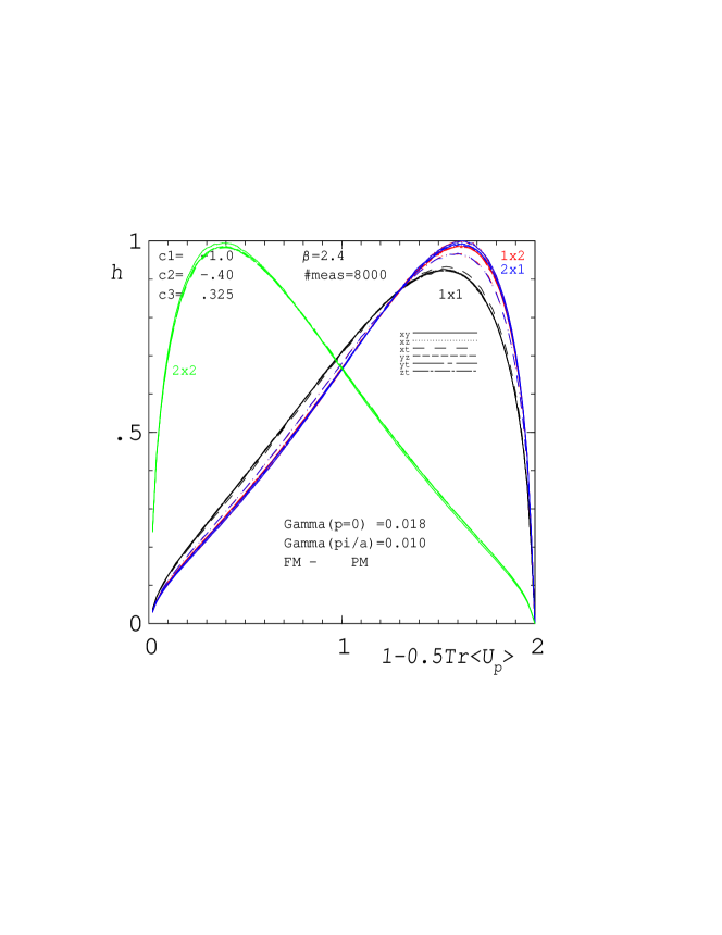
Figure 4: Histogram of Wilson loops in the action, $c_{2}=-0.4$.

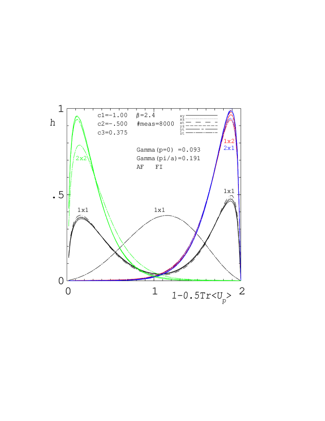
Figure 5: Histogram of Wilson loops in the action, $c_{2}=-0.5$.

One expects that the AF semi-classical vacuum can be constructed of link variables, which are elements of the center of the gauge group, analogous to a Néel state. This type of configuration satisfies the lattice equations of motion and saturates the action in the AF phase. However, in case of a mismatch between internal and external topology the competing interactions can be balanced by forming incommensurate structures [31] and the semi-classical vacuum will become even more complicated. The histogram in fig.4 shows that FM Wilson loops are concentrated around $\pm 1$ up to quantum fluctuations. This suggests a $Z_{2}$ valued semi-classical vacuum. On the contrary, AF planes also have non-center link variables $U\approx e^{i\pi\hat{n}_{j}\sigma_{j}/2}$, $\hat{n}_{j}\cdot\hat{n}_{j}=1$ demonstrated in fig.5 and the semi-classical vacuum shows a non-Abelian structure. Note that the finite value of our order parameter, given in lattice units, indicates the occurrence of an AF condensate, $<A_{\mu}>=\Lambda O(g^{-1})$, which is strong enough to modify the usual beta-function in the UV scaling regime, [42].

Figure 6: Action density for $\beta=2.4$, $c_{1}=-1.0$ as a function of $c_{2}$. The third coupling was always adjusted so that $c_{3}=1/16-c_{1}/16-c_{2}/2$. Different symbols denote contributions from the $1\times 1$, $1\times 2$ and $2\times 2$ Wilson loops to the action.

Figure 7: Total action. According to eq.10 the trivial configuration, $U_{\mu}(x)=1$, has vanishing total action. Parameter values correspond to fig.6.

The total action $S$ corresponding to fig.3 shown in fig.7 indicates that $S$ is negative, i.e. it lies below the value corresponding to the trivial vacuum, $A_{\mu}=0$, due to the negative coupling constants. Fluctuations detected by the operators, which multiply these coupling constants in the action carry negative energy and condense. The qualitative behaviour of the different terms of the action support the presence of an AF ordering with period length $2a$. In fact, the elongated, $1\times 2$ loops change sign and the $1\times 1$ plaquette average settles halfway between the maximum and minimum as we move into the new phase. At the same time the $2\times 2$ loops have a peak at the phase transition with the same asymptotic value in both phases. This indicates that the $2\times 2$ loops, which enclose two elementary cells, don’t see the AF ordering. In this case the total action became negative already before the transition.

For sufficiently large FM coupling we expect a series of phase transitions along orthogonal directions, $\hat{v}_{\alpha}$ and $\hat{w}_{\alpha}$, with increasing number of AF directions. For a fixed value of the overall coupling $\beta=4/g^{2}>0$ and $\rho=0$ the system is in the FM phase. Moving away from this point increasing $\rho$ at fixed $\beta>0$ we expect to reach a series of AF phase boundaries as the system becomes more and more frustrated. It is possible to parameterize the locations of the $n$-th phase transition as $c(\beta;~{}\rho_{n}(\beta,\phi),\phi)$. As $n$ increases more and more planes should show AF ordering. The topology of the phase boundaries is an interesting object for further investigations. It can consist of a system of concentric circles, $\rho_{n}(\beta,\phi)<\rho_{n+1}(\beta,\phi)$, or the phase boundary lines may touch each other, $\rho_{n}(\beta,\phi)=\rho_{n+1}(\beta,\phi)$ for certain $\phi$, or they can have end points. These end points might occur because the AF order depends on whether the $1\times 1$, $1\times 2$ or $2\times 2$ loop drives the instability.

First numerical evidence for a complicated topology of the phase boundary is shown in figs.4 and 5. The discontinuity of the order parameter in fig.3 suggests a first order phase transition and the distribution of the plaquette in fig.5 indicates that five planes became AF at the same critical point. It is possible that five phase boundary lines meet in this point.

7 Weak Coupling Limit

The phase transitions shown in the previous sections certainly change the infrared behaviour of the vacuum for finite value of the lattice spacing. In this section we are concerned with the AF order in the continuum limit, $a\to 0$. A complete systematical investigation of this limit is beyond the scope of this investigation which was focused on two points:

• the continuum limit is different in the AF phase than in the usual one with $c_{\alpha}=0$ and

• this difference can be understood only by assuming the existence of relevant operators different than $(F_{\mu\nu}^{a})^{2}$. This is similar to the case of the two dimensional Ising model where the the NNN coupling with AF sign is relevant in the non-homogeneous vacuum.

Let us first suppose that the system has a critical point and remains asymptotically free, i.e. the correlation length diverges for $\beta\to\infty$. The question is if the phase transitions found at finite $\beta$ persist in the limit $\beta\to\infty$?

Additional calculations of the order parameter at higher $\beta$ show the same structure as found earlier at $\beta=2.4$ (see fig. 8). At larger coupling $\beta$ the correlation $\Gamma(p)$ becomes even stronger. To confirm the stability of the transition we performed further studies, not shown in the picture, at $\beta=2.5$ on larger lattices of size $12^{4}$. Again the structure did not change and we found only very small finite size effects. Our numerical results indicate that the anti-ferromagnetic phase transition is controlled by the couplings $c_{1},c_{2}$ and $c_{3}$ almost independently from $\beta$. As a consequence it is plausible that the anti-ferromagnetic vacuum structure persists the continuum limit.

Figure 8: Comparison of the normal ($p=0$) and staggered ($p=\pi/a$) order parameter as a function of $c_{2}$ for $\beta=2.4$ (left) and $\beta=3.0$ (right), $c_{1}=-1$, and $c_{3}=1/16-c_{1}/16-c_{2}/2$. Note the different scale on the ordinates.

In the following it is instructive to look at the energy-entropy balance of SU(2) gauge theory with plaquette terms in the fundamental and adjoint representation [47]. For sufficiently large positive coefficient of the adjoint action, $\beta_{A}>\beta_{Acr}$, one finds a phase boundary separating the weak from the strong coupling regime. The transition is driven by a gas of fluxons. The fluxon gas can be constructed by first setting all link matrices to the identity and changing some of them to a non-trivial center element of the gauge group [46]. These configurations satisfy the lattice equations of motion for any action made of Wilson loops. They become unstable for $\beta_{A}<\beta_{Acr}$ [48]. Fluxons give rise to positive contributions to the action coming from the plaquette term in the fundamental representation. They are degenerate with the vacuum, $U_{\mu}(x)=1$, as far as the adjoint plaquette is concerned. The phase transition occurs when these lattice artifacts become suppressed as we approach the weak coupling regime. As a result of this suppression the phase transition has no relevance for the continuum theory.

The lesson from this generic example is that the local excitations have a chance to survive the limit, $\beta\to\infty$, if their energy does not suppress them. This is what happens in the AF phase because it occurs at negative value of the action density. Since the action density is bounded from below there must be AF solutions of the equations of motion at negative action, i.e. below the trivial vacuum, $A_{\mu}=0$. This semi-classical vacuum is highly non-trivial. The solutions of the lattice equations of motion with minimal value of the action are not yet known. It is useful to parameterize the coupling constants by polar angles $(\theta,\phi)$ of the infinite sphere $S_{2}^{c}$ as $c(\beta,\tan\theta,\phi)$ in the limit $\beta\to\infty$. Quantum fluctuations at the scale of the cut-off freeze out in this limit leaving the short range structure of the semi-classical vacuum unchanged because the modification can be expressed by a multiplicative constant in the action. According to fig.7, inhomogeneous classical solutions are energetically preferred against homogeneous ones for certain values of the parameters $\theta$ and $\phi$. Thus, the nontrivial, short-range order of the vacuum found at intermediate values of $\beta$ survives the limit $\beta\to\infty$. We expect that this change in the short range structure of the vacuum generates new phase transitions, i.e. non-analytical behaviour of densities as functions of the bare coupling constants.

According to the usual scenario there is only one relevant operator, $F^{2}_{\mu\nu}$, in four dimensional gauge theory and its coupling constant, $g^{2}$, is asymptotically free. The remaining coupling constants in eq.16 are irrelevant and may be kept constant as the cut-off is removed. The actual choice of the irrelevant coupling constants only influences the numerical value of the scale parameter, $\Lambda_{QCD}$. Our main point is that this picture is incomplete. Indeed, it also requires that the dynamics differs only by an overall scale on the FM and AF side of the phase transition on $S_{2}^{c}$. Such an equivalence between FM and AF phases is not observed even in simpler models because the two condensates couple differently to the particle modes. The difference between the phases should become even more pronounced when staggered quarks are introduced since they correspond to an AF vacuum [44] by themselves. Interactions between the excitations above the AF gauge vacuum and the staggered fermions may even be used to split the unwanted degeneracies and reduce the fermionic species doubling.

If we ask the question to what extent the usual scenario is modified by the extended action given by eq.16, the following cases are possible:

1. Renormalizable and Asymptotically Free: If asymptotic scaling prevails in the AF phase the continuum limit corresponds to $\beta=\infty$. The coupling constants, which are responsible for the AF condensate are relevant because they modify the theory by more than an overall change of scale. A higher dimensional operator may become relevant if its anomalous dimension is sufficiently negative. The lesson from the semi-classical approximation of ref. [17] is that the ratio of the coupling constants $c_{2}^{2}/c_{4}$ appears in the observables in addition to the usual polynomial terms, $c_{2}^{m}c_{4}^{n}$, arising from the perturbation expansion. This ratio which can be large even if the $c_{\alpha}$ are small may be the source of the large anomalous dimensions. The AF short distance structure of the vacuum is calculable in the framework of a saddle point expansion because $\beta$ is large. The long range order is lost due to the infrared slavery as in the integer spin AF Heisenberg chain [50]. The renormalization of the theory reveals new ultraviolet divergences due to the rapid oscillation in the semi-classical vacuum.

2. Renormalizable and Non-asymptotically Free: Due to changes in the ultraviolet structure of the theory asymptotic freedom may be lost. The continuum limit is already reached at finite value of $g^{2}$ and strong quantum fluctuations may introduce lattice defects and disorder. The vacuum is highly non-trivial both in the UV and the IR region.

3. Non-renormalizable: The model may loose all critical points in the coupling space and become non-renormalizable. It can be considered as an effective theory up to a certain scale, the UV Landau pole.

When either of these possibilities is realized a genuinely new phase of the underlying gauge theory is identified. To find out, which option is actually realized goes beyond the scope of the present paper and clearly requires further work.

8 Conclusion

We investigated the role of higher order derivatives in non-Abelian gauge theories. It was found that the relevance or irrelevance of such terms is a highly non-trivial issue, which cannot be settled on the basis of simple perturbative arguments, because higher order derivatives may enhance the contribution of configurations with characteristic scale close to the cut-off. We found numerical evidence that the semi-classical vacuum contains a condensate of modes close to the cut-off in a certain region of the coupling constant space. In this region the field strength tensor shows oscillatory behaviour and thereby displays AF, staggered ordering. We put forward an argument that at least one of the possibilities, the AF phase transition survives the removal of the cut-off or the theory looses asymptotic freedom, is realized.

The renormalization of models with an AF vacuum is highly non-trivial and cannot be covered by a simple extension of commonly used perturbative methods developed for homogeneous or slowly varying background fields. We do not, at the present, possess a procedure powerful enough to carry out the entire renormalization program. Nevertheless, we believe that the Bloch-wave formalism provides at least the framework in which this issue can ultimately be clarified. Our present result should be considered only as an indication of the possibility of constructing a new type of continuum Quantum Field Theory. A detailed analytical investigation is required to reach a comprehensive understanding of the importance of the anti-ferromagnetic vacuum structure.

The AF vacuum is generated by higher covariant derivative operators in then action. The relevance of operators depends on the global or long range structure of the vacuum. The lattice gauge theory defined by a modified plaquette action,

$$S_{\kappa}=\beta\sum_{x,\mu,\nu}\Theta\biggl{(}\kappa-{\mbox{Tr~{}}}\left(1-\raisebox{-5.69046pt}{ \begin{picture}(1.2,1.2)(-0.6,-0.6) \put(-0.5,-0.5){\line(1,0){1.0}} \put(0.5,-0.5){\line(0,1){1.0}} \put(0.5,0.5){\line(-1,0){1.0}} \put(-0.5,0.5){\line(0,-1){1.0}} \put(0.0,-0.5){\vector(1,0){0.0}} \put(0.5,0.0){\vector(0,1){0.0}} \put(0.0,0.5){\vector(-1,0){0.0}} \put(-0.5,0.0){\vector(0,-1){0.0}} \put(-0.5,-0.5){\circle*{0.2}} \put(-0.55,-0.55){\makebox(0.0,0.0)[tr]{\footnotesize$x$}} \put(-0.55,0.0){\makebox(0.0,0.0)[r]{\footnotesize$\nu$}} \put(0.0,-0.55){\makebox(0.0,0.0)[t]{\footnotesize$\mu$}} \end{picture}}\right)\biggr{)}~{}~{}{\mbox{Tr~{}}}\left(1-\raisebox{-5.69046pt}{ \begin{picture}(1.2,1.2)(-0.6,-0.6) \put(-0.5,-0.5){\line(1,0){1.0}} \put(0.5,-0.5){\line(0,1){1.0}} \put(0.5,0.5){\line(-1,0){1.0}} \put(-0.5,0.5){\line(0,-1){1.0}} \put(0.0,-0.5){\vector(1,0){0.0}} \put(0.5,0.0){\vector(0,1){0.0}} \put(0.0,0.5){\vector(-1,0){0.0}} \put(-0.5,0.0){\vector(0,-1){0.0}} \put(-0.5,-0.5){\circle*{0.2}} \put(-0.55,-0.55){\makebox(0.0,0.0)[tr]{\footnotesize$x$}} \put(-0.55,0.0){\makebox(0.0,0.0)[r]{\footnotesize$\nu$}} \put(0.0,-0.55){\makebox(0.0,0.0)[t]{\footnotesize$\mu$}} \end{picture}}\right)$$

as suggested in [51] belongs to the same universality class for any choice of the parameter $\kappa$ for $\beta>0$. This is certainly not true in the presence of higher order derivatives in the AF phase. In general, all higher order derivative terms in the action are irrelevant for the quantum fluctuations around the homogeneous vacuum, $A_{\mu}=0$. They may become relevant when the saddle point is not translation invariant [17, 41, 49].

Higher order terms of the Lagrangian are supposed to arise from the elimination of a heavy particle. The Peierls dimerisation in a 1-dimensional electron-phonon system is an example where vertices generated by a heavy fermion drive the effective theory into an AF phase. Similar phenomena may occur in higher dimensions as well [52].

This remark leads us to our last point, the striking similarity between the AF phase and solid state physics. In solid state physics, elimination of the ions generates higher order derivatives in the effective theory of photons and electrons. It is instructive to use our intuition from Solid State Physics to imagine the dynamics of excitations above an AF vacuum. It has been already mentioned that the unitarity is lost for theories with higher order derivatives. The effective theory of solids, involving electrons, photons and phonons is highly non-unitary at high energies, where ions appear as true degrees of freedom. Similarly, non-unitary aspects of the gauge theory are relevant only at energies, where AF ordering is destroyed by hard excitations.

Some well known phenomena are found in the AF phase. Consider massless QED with higher order terms in the photon action, which make the semi-classical photon vacuum AF. The electron spectrum develops forbidden zones in the spectrum due to destructive Bragg reflections. One can introduce a chemical potential for the fermion number such that the surface would be in the middle of a forbidden zone. The resulting $\gamma^{5}$ symmetrical gap in the spectrum can be interpreted as a mass gap if the level density is non-vanishing at the Fermi surface. In this way it is possible to have mass generation in a vacuum, which seems homogeneous for infrared observations. Another interesting effect may come from interactions between electrons and small fluctuations of the photon field around the inhomogeneous vacuum. Fluctuations of $A_{0}$ create the Coulomb interaction between electrons. By an appropriate fine tuning of the coupling constants of higher order terms in the action one can create an ”acoustic branch”, a massless mode of transverse photons even in the absence of a gap in the one electron spectrum. Such unscreened, long range force may be attractive and play the role of phonons in generating Cooper-pairs and super-conductivity in the vacuum.

9 Note Added

After completing the manuscript we noticed a preprint with similar starting point but different goals [53].

10 Acknowledgment

We thank V. Branchina, D. Dyakonov, J. Jersák and H. Mohrbach for useful discussions.

References

-
[1]
K.G. Wilson, J. Kogut, Phys. Rep. 12C (1974) 75;
K.G. Wilson, Rev. Mod. Phys. 47 (1975) 773; Rev. Mod. Phys. 55 (1983) 583. - [2] A. Hasenfratz and P. Hasenfratz, Ann. Rev. Nucl. Part. Sci. 35 (1985) 559.
- [3] S.B. Liao, J. Polonyi, Phys. Rev. D51 (1955) 4474.
-
[4]
P.I. Fomin, V.P. Gusynin and V.A. Miranskii, Phys. Rev. 78B (1978) 136;
V.A. Miranskii, Phys. Lett. 91B (1980) 421; Nucl. Phys. 90A (1985) 149;
V.A. Miranskii, Dynamical Symmetry Breaking in Quantum Field Theories, Singapore, World Scientific, (1994). - [5] C.N. Leung, S.T. Love and W.A. Bardeen, Nucl. Phys. B273 (1986) 649.
- [6] S. Caracciolo, R.G. Edwards, A. Pelissetto and A.D. Sokal, Nucl. Phys. B30 (Proc. Suppl.) (1993) 815.
- [7] H.G. Ballesteros, L.A. Fernández, V. Martin-Mayor and A. Munoz Sudupe, New Universality Class in three dimensions: the Antiferromagnetic model, e-Print Archive: hep-lat/9511003.
- [8] M. Hasenbusch, and Models in Two Dimensions, e-Print Archive: hep-lat/9507008.
- [9] F. Niedermayer, P. Weisz and Dong-Shin Shin, On the question of universality in and Lattice Sigma Models, e-Print Archive: hep-lat/9507005.
-
[10]
C. Frick and J. Jersák, Phys. Rev. D52 (1995) 340;
E. Focht, J. Jersák and J. Paul, Magnetic and chiral universality classes in a 3D Yukawa model, e-Print Archive: hep-lat/9509040. -
[11]
H. Neuberger, University of Tel-Aviv thesis (1976);
M. Bander, Univ. Calif. Irvine, Preprint (1975);
M. Halpern, Phys. Rev. D12 (1975) 1684;
H. Lehmann and J. Stehr, The Bose Field Structure associated with a free massive Dirac Field in one space Dimension, DESY Preprint, 76/29, June 1976;
B. Schroer and T. Truong, Phys. Rev. D15 (1977) 1684. - [12] K. Huang and J. Polonyi, J. Mod. Phys. A6 (1991) 409.
- [13] T. Reisz, Comm. Math. Phys. 116 (1988) 81, 573; 117 (1988) 79; Nucl. Phys. B318 (1989) 417.
- [14] J. Zinn-Justin, Quantum Field Theory and Critical Phenomena, Clarendon Press, Oxford (1979).
- [15] T.D. Bakeyev and A.A. Slavnov, Higher Covariant Derivative Regularization Revisited, e-Print Archive: hep-th/9601092.
-
[16]
T. Appelquist and J. Carazzone, Phys. Rev. D11 (1975) 2856;
T. Appelquist, J. Carazzone, H. Kluberg-Stern, M. Roth, Phys. Rev. Lett. 36 (1976) 768, 1161;
T. Appelquist and J. Carazzone, Nucl. Phys. B120 (1977) 77. - [17] V. Branchina, J. Polonyi, Nucl. Phys. B433 (1995) 99.
-
[18]
M. Lüscher, Nucl. Phys. B200 (1982) 61;
J. Polonyi, Phys. Rev. D29 (1984) 716. -
[19]
Y. Iwasaki and T. Yoshie, Phys. Lett. 130B (1983) 77;
S. Itoh, Y. Iwasaki and T. Yoshie, Phys. Lett. 147B (1984) 141. -
[20]
M. Lüscher, Comm. Math. Phys. 85 (1982) 39;
A. Phillips and D. Stone, Comm. Math. Phys. 103 (1986) 599;
J. Hoek, M. Teper and J. Waterhouse, Nucl. Phys. B288 (1987) 589. - [21] L.S. Schulman, Techiques and Applications of Path Integration, New York, Addison-Wesley, 1981.
- [22] J. Polonyi, Renormalization Group in Quantum Mechanics, Nucl. Phys. B42 (Proc. Suppl.) (1995) 926.
- [23] J. Polonyi, Contribution to Workshop on Quantum Infrared Physics, Paris, France, 6-10 June 1994, e-Print Archive: hep-th/9411215.
-
[24]
P. Hasenfratz and F. Niedermayer, Nucl. Phys. B414 (1994) 785;
T. DeGrand, A. Hasenfratz, P. Hasenfratz and F. Niedermayer, Nucl. Phys. B454 (1995) 587. - [25] M. Lüscher and P. Weisz, Comm. Math. Phys. 97 (1985) 59; [Erratum: 98 (1985) 443].
- [26] C.J. Morningstar, Phys. Rev. D48 (1993) 2265.
-
[27]
M. García Pérez, A. Gonzáles-Arroyo, J. Snippe and P. van Baal,
Nucl. Phys. B413 (1994) 535;
M. García Pérez, J. Snippe and P. van Baal, Testing Improved Actions, e-Print Archive: hep-lat/9607007. - [28] B. Beinlich, F. Karsch and E. Laermann, Nucl. Phys. B462 (1996) 415.
- [29] K. Symanzik, Nucl. Phys. B226 (1983) 187, 205.
- [30] M. Lüscher and P. Weisz, Phys. Lett. B158 (1985) 250.
- [31] W. Selke in Phase Transitions and Critical Phenomena, eds. C. Domb and J.L. Lebowitz, Academic Press, London (1992).
-
[32]
J.L. Alonso, et al.,
Non-classical exponents in the d=4 Ising model with
two couplings, e-Print Archive: hep-lat/9503016,
I. Campos, L.A. Fernandez and A. Tarancon, Antiferromagnetic 4-d O(4) Model, e-Print Archive: hep-lat/9606017. - [33] G. Parisi and J.J. Ruiz-Lorenzo, On the Four Dimensional Diluted Ising Model, e-Print Archive: cond-mat/9503016.
-
[34]
S. Caracciolo and S. Paternello, Phys. Lett. A126 (1988) 233;
M. Bernashi et al., Phys. Lett. B231 (1989) 157;
L.A. Fernandez et al., Phys. Lett. B217 (1989) 314;
R.V. Gavai and F. Karsch, Phys. Rev. B46 (1992) 944;
S.J. Ferreira and A.D. Sokal, Antiferromagnetic Potts Model on the Square Lattice, e-Print Archive: hep-lat/9405015. - [35] G. Gallavotti and V. Rivasseau, Phys. Lett. 122B (1983) 268.
- [36] K. Osterwalder and R. Schrader, Comm. Math. Phys. 31 (1973) 83; K. Osterwalder end E. Seiler, Ann. Phys. 110 (1978) 440.
- [37] A. Pais, G.E. Uhlenbeck, Phys. Rev. 79 (1950) 145.
- [38] T.D. Lee, G.C. Wick, Nucl. Phys. B9 (1969) 209; Phys. Rev. D2 (1970) 1033.
- [39] C. Liu, K. Jansen and J. Kuti, Nucl. Phys. B34 (Proc. Suppl.) (1994) 635; Nucl. Phys. B42 (Proc. Suppl.) (1995) 630.
- [40] Chung-I Tan and Zai-Xin Xi, Phys. Rev. D30 (1984) 455.
-
[41]
M. Nauenberg, B. Nienhuis, Phys. Rev. Lett. 33 (1974) 944;
Phys. Rev. Lett. 35 (1975) 477;
J.M.J. van Leeuwen, Phys. Rev. Lett. 34 (1975) 1056;
R.H. Swendsen, S. Krinsky, Phys. Rev. Lett. 43 (1979) 177;
S. Caracciolo, S. Paternello, Phys. Lett. A126 (1988) 233; - [42] J. Magnen, V. Rivasseau and R. Sénéor, Phys. Lett. B283 (1992) 90; Comm. Math. Phys. 155 (1993) 326.
- [43] V. A. Alessandrini, H. J. de Vega and F. Schaposnik, Phys. Rev. B10 (1974) 3906; B12 (1975) 5034.
-
[44]
E. Langmann and G.W. Semenoff, Phys. Lett. B297 (1992) 175;
M.C. Diamantini, P. Sodano, E. Langmann and G.W. Semenoff, Nucl. Phys. B406 (1993) 595. - [45] V. Branchina, H. Mohrbach and J. Polonyi, in preparation.
- [46] I.G. Halliday and A. Schwimmer, Phys. Lett. 101B (1981) 327.
-
[47]
G. Bhanot, M. Creutz, Phys. Rev. D24 (1981) 3212;
R. Dashen, U.M. Heller and H. Neuberger, Nucl. Phys. B215 (1983) 380. - [48] G. Bhanot, R. Dashen, Phys. Lett. 113B (1982) 299.
-
[49]
M. Bernaschi et al. Phys. Lett. B231 (1989) 157;
L.A. Fernandez et al. Phys. Lett. B217 (1989) 314. - [50] E. Fradkin, Field Theories of Condensed Matter Systems, Addison-Wesley, 1991.
- [51] J. Fingberg, U.M. Heller and V. Mitryushkin, Nucl. Phys. B435 (1995) 311.
- [52] V. Branchina, J. Polonyi, in preparation.
- [53] Y. Shamir, The Standard Model from a New Phase Transition on the Lattice, e-Print Archive: hep-lat/9512019.