The Kosterlitz–Thouless Universality Class

Abstract

We examine the Kosterlitz–Thouless universality class and show that essential scaling at this type of phase transition is not self–consistent unless multiplicative logarithmic corrections are included. In the case of specific heat these logarithmic corrections are identified analytically. To identify those corresponding to the susceptibility we set up a numerical method involving the finite–size scaling of Lee–Yang zeroes. We also study the density of zeroes and introduce a new concept called index scaling. We apply the method to the $XY$–model and the closely related step model in two dimensions. The critical parameters (including logarithmic corrections) of the step model are compatable with those of the $XY$–model indicating that both models belong to the same universality class. This result then raises questions over how a vortex binding scenario can be the driving mechanism for the phase transition. Furthermore, the logarithmic corrections identified numerically by our methods of fitting are not in agreement with the renormalization group predictions of Kosterlitz and Thouless.

1 Introduction

In lattice field theory one is interested in the phenomenon of phase transitions, where the quantity representing the length scale of relevant physics (correlation length or inverse mass gap) diverges. Typically, in spin models, the transition is between phases with and without long range order. In models with a temperature driven phase transition these phases are distinguished by negative and positive reduced temperature ($t$) respectively. A conventional phase transition is then characterised by a power–law divergence in the (infinite volume) correlation length near criticality (near $t=0$);

$$\xi_{\infty}\sim\mid t\mid^{-\nu}\quad.$$ (1.1)

1.1 The $XY$–Model

In two dimensional spin models with continuous symmetry group and continuous interaction Hamiltonian, the existence of a phase with conventional long range order is precluded by the Mermin–Wagner theorem [2]. Therefore there is no spontaneous magnetisation in $O(n)$–spin models for $n\geq 2$. Physically, the reason for this is that any long range order which would otherwise be present is destroyed by spin wave excitations in two dimensions.

In such models there can however exist topological long range order. Indeed, in a $d$-dimensional theory, if the order parameter lies in a space $G$, then topological defects of dimension $p$ can occur if the $(d-p-1)^{\rm{th}}$ homotopy group $\pi_{d-p-1}(G)$ is non trivial [3]. Thus the two dimensional $O(2)$–model can have point defects or vortices.

Kosterlitz and Thouless used approximate renormalization group [RG] methods to show the existence of a phase transition driven by the binding of such vortices in the two dimensional $XY$–model (which is also called the $O(2)$ non-linear $\sigma$–model or the two component Heisenberg model) at finite non-zero temperature [4, 5]. The two dimensional $XY$–model remains the generic model for the study of Kosterlitz–Thouless [KT] type phase transitions.

The partition function for the classical $n$–component Heisenberg model on a lattice $\Lambda$ of linear extent $L$ is

$$Z_{L}(\beta,h)=\int_{S_{n-1}}{\prod_{x\in\Lambda}{d{\vec{\sigma}}_{x}e^{\beta S+{\vec{h}}.{\vec{M}}}}}\quad,$$ (1.2)

where

$$S=\sum_{x\in\Lambda}\sum_{\mu=1}^{d}{\vec{\sigma}}_{x}.{\vec{\sigma}}_{x+\mu}\quad,\quad\quad{\vec{M}}=\sum_{x\in\Lambda}{\vec{\sigma}}_{x}\quad,$$ (1.3)

and where $\beta=1/kT$ is the (reduced) inverse temperature ($T$ being the temperature and $k$ the Boltzmann constant). The $n$–component spins ${\vec{\sigma}}_{x}$ have unit modulus and ${\vec{h}}$ is a (reduced) external field. This is the infinite bare coupling limit of the $O(n)$ $\phi^{4}$–model. It is believed that the $n$–component Heisenberg model is in the same universality class as the general $O(n)$ $\phi^{4}$–model.

The scenario proposed by Berezinskii [4] and Kosterlitz and Thouless [5] is that at temperatures above some critical value ($\beta<\beta_{c}$) the vortices and antivortices are unbounded and serve to disorder the system. The vortex chemical potential is a relevant variable. Decreasing the temperature ($\beta\nearrow\beta_{c}$) causes the vortices and antivortices to bind, thereby decreasing their relevance as dynamical degrees of freedom. The model remains critical (thermodynamic functions diverge) for all $\beta>\beta_{c}$ and the critical exponents are dependent on temperature. In terms of the reduced temperature, which is defined as

$$t=1-\frac{\beta}{\beta_{c}}\quad,$$ (1.4)

the leading critical behaviour of the correlation length, susceptibility and the specific heat is given in [5] as

$$\xi_{\infty}(\beta) \sim e^{bt^{-\nu}}\quad,$$ (1.5)

$$\chi_{\infty}(\beta) \sim \xi_{\infty}^{\tilde{\gamma}}\quad,$$ (1.6)

$$C_{\infty}(\beta) \sim \xi_{\infty}^{\tilde{\alpha}}+{\rm{constant}}\quad,$$ (1.7)

where for $t\rightarrow 0^{+}$, $\nu=1/2$, $\tilde{\gamma}=\gamma/\nu=2-\eta_{c}=7/4$ and $\tilde{\alpha}=\alpha/\nu=-d=-2$.

The exponential scaling behaviour of (1.5) is referred to as essential scaling to distinguish it from the (more usual) power-law behaviour of (1.1). Thus the ‘KT scenario’ means a phase transition (i) driven by a vortex binding mechanism and (ii) exhibiting essential scaling behaviour.

Although essential scaling is also often referred to as KT scaling, this (exponential) scenario was known to exist in certain models before the seminal work of [5]. In particular, the BCSOS and F- models are special cases of the $6$–vertex model and are exactly solvable in the absence of an external field [6]. This means that the even thermodynamic functions and in particular the free energy and the correlation length are exactly obtainable in these models. The latter has the form (1.5) (also with $\nu=1/2$) and the singular part of the free energy is

$$f^{\rm{BCSOS}}_{\infty}(\beta)\propto\xi_{\infty}^{-2}\quad.$$ (1.8)

This model has not been solved in the presence of an external field and the odd critical exponents ($\gamma$, $\eta$ and $\delta$) are not, therefore, rigorously determinable. (Neither are these critical exponents determinable from the usual scaling relations since they don’t all hold in the case of an essential critical point [5, 6]).

The reasoning presented by KT supporting an essential scaling scenario for the $XY$–model (see also [7, 8, 9, 10]) is non–rigorous and a primary concern of lattice (non-perturbative) field theory has been its verification. An unambiguous verification of all the KT predictions has until now however proved elusive. Recently, however, Hasenbusch et al. [11] numerically matched the RG trajectory of the dual of the $XY$–model to that of the BCSOS model. This provides further evidence that at least the even critical exponents of the $XY$–model are those given by KT.

Most Monte Carlo [MC] and high temperature expansion [TE] analyses of the $XY$–model have concentrated on the numerical determination of $\nu$ and $\eta$ from (1.5) and (1.6) as they stand. These determinations are notoriously difficult not least because multi-parameter fits are required. Commonly, $\beta_{c}$ is determined by fixing $\nu=1/2$ in (1.5). Typically, however, the subsequent fit to (1.6) yields a value significantly different from the KT prediction $\eta_{c}=1/4$. Unconstrained four-parameter fits are hampered by slow convergence problems due to extremely shallow valleys in the 4–parameter space [12] and also fail in general to quantitatively and unambiguously confirm the KT predictions. Table 1 demonstrates this by listing some of the more recent estimates for $\beta_{c}$ and $\eta_{c}$ from Monte Carlo [MC] and high temperature expansion [TE] methods.

Table 1: Estimates for $\beta_{c}$ and $\eta_{c}$ for the $XY$–model from a selection of papers. Those marked with an asterisk favour conventional as opposed to essential scaling behaviour.

Authors	Year	Method	$\beta_{c}$	$\eta_{c}$
Fernández et al. [13]	1986	MC (FSS)	$1.1$	$0.24(3)$
Seiler et al. [14] $~{}^{*}$	1988	MC	$1.01(1)$	$0.38(2)$
Gupta et al. [12]	1988	MC	$1.114(2)$	$0.34$
Wolff [15]	1989	MC	$1.12(7)$	$0.280(4)$
Biferale, Petronzio [16]	1989	MC(FSS)	$1.112(2)$	0.243(7)
Butera, Comi,Marchesini [17]	1989	TE	$1.112(6)$	0.300(25)
Ferer, Mo [18]	1990	MC(BSRG)	$1.115(10)$	$0.27(3)$
Hulsebos, Smit, Vink [19]	1990	MC(FSS)	$1.13$
Edwards, Goodman, Sokal [20]	1991	MC(FSS)	$1.130(15)$
Gupta, Baille [21]	1991	MCRG(FSS)	$1.119(5)$	$0.235(5)$
Butera, Comi [22]	1993	TE	$1.118(3)$	$0.27(2)$
Janke, Nather [23]	1993	MC(FSS)		$0.2389(6)$
Catterall, Kogut, Renken [24]	1993	MC(FSS)		$0.247(1)$
Butera, Comi [25]	1994	TE		$0.27(1)$
Schultka, Manousakis [26]	1994	MC(FSS)	$1.119(4)$
Hasenbusch, Marcu, Pinn [11]	1994	MC(BSRG)	$1.1197(5)$
Olsson [27]	1995	MC	$1.1209(1)$
Kim [28] $~{}^{*}$	1995	MC	$1.108(3)$
Campostrini et al. [29]	1995	TE	$1.118(4)$	$0.228(1)$

In a recent letter [30] we presented a very general theoretical argument showing that the essential scaling scenario is not self–consistent unless multiplicative logarithmic corrections are included. We believe that the measured values of $\eta_{c}$ in table 1 deviate from the theoretical value ($\eta_{c}=1/4$) because these logarithmic corrections have been ignored in these analyses (the only exception being [22]). Our assertion is that it is essential to take account of the possibility of multiplicative logarithmic corrections in any attempt to numerically verify an essential scaling scenario.

In [30] we also presented a new method involving the finite–size scaling [FSS] of the first Lee–Yang zero [31] whereby the critical point $\beta_{c}$ and the leading and logarithmic correction critical indices can be determined numerically from two parameter (straight line) fits. Here we wish to elaborate on these theoretical and numerical approaches and to extend our analysis to the first ten Lee–Yang zeroes.

1.2 The step Model

The step model or sgn $O(2)$ model is closely related to the $XY$–model [32, 33, 34, 35]. Its partition function is given by (1.2) with

$$S^{\rm{step}}=\sum_{x\in\Lambda}\sum_{\mu=1}^{d}\hbox{sgn}({\vec{\sigma}}_{x}\cdot{\vec{\sigma}}_{x+\mu})\quad.$$ (1.9)

The question of criticality of this model has, until now, been unresolved despite several analyses based on high temperature series and on numerical simulation [36, 37]. The interest in the model arises from its possible membership of the Kosterlitz–Thouless universality class. Like the $XY$–model, the step model has a configuration space which is globally and continuously symmetric. Unlike the $XY$–model, however, the interaction function is discontinuous and the Mermin–Wagner theorem [2] remains unproven for this case (see however [38]). Nonetheless, it is expected that if a phase transition exists in the step model, it should not be to a phase with long range order [33, 37, 39].

The KT phase transition of the $XY$–model is understood to be driven by the binding/unbinding of vortices. The energetics of vortex formation in the step model are, however, very different from the $XY$–model [35, 37, 39]. Since vortices with effectively zero excitation energy can be created at all non-zero temperatures, the usual KT argument does not naturally lead one to expect such a phase transition in the step model.

Sánchez–Velasco and Wills [37] presented evidence of critical behaviour starting at $\beta_{c}^{\rm{step}}=0.91\pm 0.04$. This was based on FSS of the spin susceptibility. Since the associated critical index $\eta(\beta_{c}^{\rm{step}})$ was significantly greater than that measured for the $XY$–model, it was concluded that the step and $XY$ models are not in the same universality class. In this paper we present evidence that the step model is not in fact critical at that temperature. However it is critical at lower temperatures with a critical index $\eta(\beta_{c}^{\rm{step}})$ compatible with the $XY$ value.

These results are consistent with the possibility that the $XY$– and step models belong to the one universality class. Since the KT vortex unbinding mechanism is not believed to be responsible for the phase transition of the step model, the same scenario has to be questioned in the $XY$–model. This is not the first time the KT scenario has been questoned. For earlier counter-evidence to both the physical KT picture as well as the quantitative essential scaling predictions see [41, 42, 43] and [14, 40]. Further criticisms of the conventional view are found in [44].

The accuracy afforded by the Lee–Yang zeroes study and the consideration of multiplicative logarithmic corrections are essential for the present analysis [45].

2 Lee–Yang Zeroes and Logarithmic Corrections to Scaling

The subject of partition function zeroes was introduced in 1952 by Lee and Yang [31] as an alternative way to understand the onset of criticality in statistical physics models. For a finite system the zeroes of the partition function are strictly complex (non–real). As $L$ is allowed to go to infinity one generally expects these zeroes to condense onto smooth curves. Zeroes in the plane of complex external magnetic field $h$ are refered to as Lee–Yang zeroes. Lee and Yang further showed that for certain Ising–type systems these zeroes are in fact restricted to the imaginary $h$ axis (the Lee–Yang theorem) [31]. Dunlop and Newman proved that the Lee–Yang theorem holds for the two dimensional $XY$–model [46]. While no specific proof exists for the step model, its similarities to the $XY$–model lead one to anticipate a similar locus of zeroes. In practice, one obtains numerical confirmation of this hypothesis by explicit determination of the locus.

In the symmetric phase, $t>0$, the Lee–Yang zeroes lie away from the real $h$-axis, pinching it only as $t\searrow 0$ (in the thermodynamic limit). For systems obeying the Lee–Yang theorem this pinching occurs at $h=0$, prohibiting analytic continuation from ${\rm{Re}}(h)<0$ to ${\rm{Re}}(h)>0$.

2.1 Lee–Yang Zeroes

Consider a partition function of the form

$$Z_{L}(\beta,h)=\frac{1}{{\cal{N}}_{L}}\sum_{\{\vec{\sigma}_{x}\}}{e^{\beta S+h{\hat{n}}.{\vec{M}}}}\quad,$$ (2.1)

where ${\hat{n}}$ is a unit vector defining the direction of the external magnetic field and $h$ is a scalar parameter representing its strength. The factor ${{\cal{N}}_{L}}$ ensures that $Z_{L}(0,0)=1$. Here $S$ and ${\vec{M}}$ are given by (1.3) or (1.9), $S$ taking real values from the interval $[-dL^{d},dL^{d}]$ ($dL^{d}$ is the number of links in $\Lambda$) and $M=(\hat{n}.\vec{M})$ taking the real values in $[-L^{d},L^{d}]$ ($L^{d}$ being the number of sites in $\Lambda$).

Suppose now that the $M$–range is binned such that there are $2N_{M}$ $M$–bins of width $\Delta_{M}={L^{d}}/{N_{M}}$. Defining the integrated spectral density $\rho_{L,\beta}^{(\Delta)}(M)$ as the number of configurations having given $M$– values, the partition function for this system can be written as

$$Z_{L}^{(\Delta)}(\beta,h)=\frac{e^{-hM_{\rm{max}}}}{{\cal{N}}^{(\Delta)}_{L}}\sum_{k=0}^{2M_{\rm{max}}/\Delta_{M}}{\rho_{L,\beta}^{(\Delta)}\left(k\Delta_{M}-M_{\rm{max}}\right)\left(e^{h\Delta_{M}}\right)^{k}}\quad,$$ (2.2)

where $M_{\rm{max}}=(N_{M}-\frac{1}{2})\Delta_{M}$ and where $k\in{{\mbox{\math N}}}$ and ${\cal{N}}^{(\Delta)}_{L}$ is such that $Z_{L}^{(\Delta)}(0,0)=1$. Thus $Z_{L}^{(\Delta)}(\beta,h)$ is proportional to a polynomial with real coefficients of order $2M_{\rm{max}}/\Delta_{M}$ in the ‘fugacity’ $z=\exp{(h\Delta_{M})}$ and as such has $2M_{\rm{max}}/\Delta_{M}$ zeroes in the complex $z$–plane.

For the Ising model (for example) $\Delta_{M}$ is the minimum change in the total magnetization upon flipping a single spin. There $\Delta_{M}=2$. In the $XY$–model the $M$–range is continuous, even for a finite system. However, when we come to the numerical analysis of the $XY$–model, the Monte Carlo integration method can only sample a discrete subset of the infinite range of configurations open to the system. It thus accesses only a discrete sample of $M$–values from the range $[-L^{d},L^{d}]$. If no binning is used in the numerical approach, then the minimum separation between two such $M$–values will play the rôle of $\Delta_{M}$ above. In any case, the partition function is still proportional to a polynomial in the fugacity. The real and imaginary parts of the partition function are separately periodic in ${\rm{Im}}(h)$ with period $2\pi/\Delta_{M}$. The pattern of Lee–Yang zeroes is itself therefore periodic in ${\rm{Im}}(h)$ with the same period.

2.2 Scaling and Corrections to scaling

Assume that the Lee–Yang theorem holds for the binned system. In terms of its zeroes,

$$z_{j}(\beta,L)=e^{i\Delta_{M}\theta_{j}(\beta,L)}\quad,$$ (2.3)

the partition function (2.2) is

$$Z_{L}^{(\Delta)}(\beta,h)=\frac{e^{-hM_{\rm{max}}}}{{\cal{N}}^{(\Delta)}_{L}}\rho_{L,\beta}^{(\Delta)}\left(M_{\rm{max}}\right)\prod_{j=1}^{2M_{\rm{max}}/\Delta_{M}}\left(z-z_{j}(\beta,L)\right)\quad.$$ (2.4)

Assume

$$f_{L}(\beta,h)=\lim_{\Delta_{M}\rightarrow 0}{f_{L}^{(\Delta)}(\beta,h)}=\lim_{\Delta_{M}\rightarrow 0}{L^{-d}\ln{Z_{L}^{(\Delta)}(\beta,h)}}\quad.$$ (2.5)

Zeroes on the unit circle in the complex fugacity plane correspond to zeroes on the imaginary $h$ axis. Following [50, 51, 52], we define the density of these zeroes as

$$g_{L}(\beta,\theta)=\frac{dG_{L}(\beta,\theta)}{d\theta}=L^{-d}\sum_{j=1}^{2M_{\rm{max}}}{\delta(\theta-\theta_{j}(\beta,L))}\quad.$$ (2.6)

Scaling in the Thermodynamic Limit

Using the symmetry and periodicity [30] of the pattern of zeroes one finds for the the free energy in the thermodynamic limit [47]

$$f_{\infty}(\beta,h)=f_{\rm{reg}}(\beta,h)-2\int_{\theta_{c}}^{\infty}{\frac{\theta}{h^{2}+\theta^{2}}G_{\infty}(\beta,\theta)d\theta}\quad.$$ (2.7)

where $\theta_{c}(\beta)$ is the Yang–Lee edge and is given by [48, 49]

$$g_{\infty}(\beta,\theta)=0{\rm{~{}~{}for~{}~{}}}-\theta_{c}(\beta)<\theta<\theta_{c}(\beta)\quad.$$ (2.8)

The zero field susceptibility is the second derivative of the free energy with respect to $h$,

$$\chi_{\infty}(\beta)=\left.\frac{\partial^{2}f_{\infty}}{\partial h^{2}}\right|_{h=0}=4\int_{\theta_{c}(\beta)}^{\infty}\theta^{-3}G_{\infty}(\beta,\theta)d\theta\quad.$$ (2.9)

Following [50, 51, 52, 30], the cumulative density of zeroes can be written in terms of the susceptibility and the Yang–Lee edge:

$$G_{\infty}(\beta,\theta)=\chi_{\infty}(\beta){(\theta_{c}(\beta))}^{2}\Phi\left(\frac{\theta}{\theta_{c}(\beta)}\right)\quad,$$ (2.10)

$\Phi(x)$ being some function of $x$ with $\Phi(\mid x\mid\leq 1)=0$.

The (singular part of the) specific heat is then

$$C^{\rm{sing}}_{\infty}(\beta)=\left.\frac{\partial^{2}f^{\rm{sing}}_{\infty}(\beta,h)}{\partial\beta^{2}}\right|_{h=0}=-2\int_{\theta_{c}(\beta)}^{\infty}\theta^{-1}\frac{d^{2}G_{\infty}\left(\beta,\theta\right)}{d\beta^{2}}d\theta\quad.$$ (2.11)

The above formulae are quite general and hold for any model provided only that it obeys the Lee–Yang theorem. To proceed from here we have to insert the (model–specific) critical behaviour. Instead of the conventional KT formula (1.6) and (1.7) assume, now, the following more general behaviour for the zero field susceptibility, the edge and for the singular part of the specific heat

$$\chi_{\infty}(\beta) \sim \xi_{\infty}^{\tilde{\gamma}}(\ln{\xi_{\infty}})^{\tilde{r}}\quad,$$ (2.12)

$$\theta_{c}(\beta) \sim \xi_{\infty}^{\lambda}(\ln{\xi_{\infty}})^{\tilde{p}}\quad,$$ (2.13)

$$C^{\rm{sing}}_{\infty}(\beta) \sim \xi_{\infty}^{\tilde{\alpha}}(\ln{\xi_{\infty}})^{\tilde{q}}\quad,$$ (2.14)

and

$$\gamma = \nu\tilde{\gamma}\quad\quad\quad\quad r=-\nu\tilde{r}\quad$$ (2.15)

$$\alpha = \nu\tilde{\alpha}\quad\quad\quad\quad q=-\nu\tilde{q}\quad.$$ (2.16)

Then (2.10) and (2.11) give

$$\xi_{\infty}^{\tilde{\alpha}-\tilde{\gamma}-2\lambda}(\ln{\xi_{\infty}})^{\tilde{q}-\tilde{r}-2\tilde{p}}\propto\left[c_{1}\frac{\ddot{\xi}_{\infty}}{\xi_{\infty}}+c_{2}\left(\frac{\dot{\xi}_{\infty}}{\xi_{\infty}}\right)^{2}\right]\left\{1+O\left(\frac{1}{\ln{\xi_{\infty}}}\right)\right\}\quad.$$ (2.17)

Inserting the leading KT behaviour for the correlation length (1.5) gives

$$\tilde{\alpha}=\tilde{\gamma}+2\lambda\quad,$$ (2.18)

and

$$\tilde{q}=\tilde{r}+2\tilde{p}+2\left(1+\frac{1}{\nu}\right)\quad.$$ (2.19)

Here we have the first indications that KT scaling behavoiur (1.5) – (1.7) is not self–consistent without multiplicative logarithmic corrections. If there are no logarithmic corrections then $\tilde{q}=\tilde{r}=\tilde{p}=0$ and (2.19) cannot hold.

Finite–Size Scaling

The finite–size scaling (FSS) hypothesis, first formulated in 1971 by Fisher and co-workers [53], is a relationship between the critical behaviour of thermodynamic quantities in the infinite volume limit and the size dependency of their finite volume counterparts. The general statement of FSS, which is expected to hold in all dimensions [54] is that if $P_{L}(\beta)$ is the value of some thermodynamic quantity $P$ at inverse temperature (coupling) $\beta$ measured on a system of linear extent $L$, then

$$\frac{P_{L}(\beta_{c})}{P_{\infty}(\beta)}={\cal{F}}_{P}\left(\frac{\xi_{L}(\beta_{c})}{\xi_{\infty}(\beta)}\right)\quad,$$ (2.20)

where $\xi_{L}(\beta)$ is the correlation length of the finite–size system. Here ${\cal{F}}_{P}$ is some $P$–dependent function of the scaling variable $x=\xi_{L}(\beta_{c})/\xi_{\infty}(\beta)$. Fixing the scaling variable, one has

$$\xi_{\infty}(\beta)\sim x^{-1}\xi_{L}(\beta_{c})\quad.$$ (2.21)

Luck has shown that for the two dimensional $XY$ model, $\xi_{L}(\beta_{c})$ is proportional to $L$ [55]. Therefore FSS for the susceptibility and the Yang–Lee edge is from (2.12) and (2.13)

$$\chi_{L}(\beta_{c}) \sim L^{\tilde{\gamma}}(\ln{L})^{\tilde{r}}$$ (2.22)

$$\theta_{1}(\beta_{c}) \sim L^{\lambda}(\ln{L})^{\tilde{p}}\quad.$$ (2.23)

Now, from (2.4) and (2.7) the magnetic susceptibility for a finite–size system is

$$\chi_{L}(\beta)=\left.\frac{\partial^{2}f_{L}}{\partial h^{2}}\right|_{h=0}=-L^{d}\sum_{j}{\frac{1}{\theta_{j}^{2}}}\quad.$$ (2.24)

If the lowest lying zeroes exhibit the same FSS behaviour [56], then

$$\chi_{L}(\beta)\sim-L^{-d}\theta_{1}(\beta)^{-2}\quad.$$ (2.25)

We provide numerical justification for this assumption in Sec. 4.1. Together, (2.22), (2.23) and (2.25) give

$$\lambda = -\frac{1}{2}(d+\tilde{\gamma})\quad,$$ (2.26)

$$\tilde{p} = -\frac{1}{2}\tilde{r}\quad,$$ (2.27)

whence

$$\tilde{\alpha}=-d\quad,$$ (2.28)

and

$$\tilde{q}=2\left(1+\frac{1}{\nu}\right)\quad.$$ (2.29)

Thus the KT result for the leading specific heat index $\alpha$ is recovered. However the correction index is $q=2(\nu+1)=3$, a non-trivial result. There are therefore multiplicative logarithmic corrections to the leading (KT) scaling behaviour of the singular part of the specific heat.

$$C^{\rm{sing}}_{\infty}\sim\xi_{\infty}^{-2}(\ln{\xi_{\infty}})^{6}\sim\xi_{\infty}^{-2}t^{-3}\quad.$$ (2.30)

The full specific heat has another (constant) term coming from the regular part of the free energy and since the leading critical index is negative any numerical verification of (2.30) is rendered very difficult if not impossible [57].

Integrating (2.30) twice with respect to $t$ gives the singular part of the free energy to be $f_{\infty}\sim\xi_{\infty}^{-2}$ as in (1.8). Thus we have indirectly verified hyperscaling for the two-dimensional $XY$–model and we have done this using the self-consistency of the essential scaling behaviour and finite–size scaling.

The above analytic considerations have yielded no information on the odd correction exponent $r$. The original renormalisation group analysis of Kosterlitz and Thouless [5], in fact, implicitly contained the prediction

$$r=-1/16$$ (2.31)

as noted by [22]. Subsequent analyses have concentrated on the $r=0$ form of the scaling behaviour (2.22) and the verification that $\eta(\beta_{c})=1/4$. Allton and Hamer [58] have conjectured that the deviation of their determination of $\eta$ from $1/4$ might be due to logarithmic corrections.

With $\nu=1/2$ and $\lambda=-2+\eta_{c}/2$ the FSS formula for the first Lee–Yang zero is

$$\theta_{1}(\beta_{c})\sim L^{\lambda}(\ln{L})^{r}\quad.$$ (2.32)

The study of this full scaling form and the numerical determination of $r$ is the subject of what follows.

3 Numerical Results

The Monte Carlo (MC) method is a stochastic method of importance sampling and an intrinsically non–perturbative approach to the calculation of path integrals and expectation values. In this section we wish to report on an application to the $XY$–model in an attempt to test independently the above scaling scenario.

In recent years the development of more efficient techniques has enhanced the quality and practicality of certain numerical calculations in bosonic spin systems. These improvements include

$\bullet$ the advent of non–local algorithms [15, 59] which greatly reduce critical slowing down,

$\bullet$ the rediscovery and development of the spectral density method which allows extrapolation away from the simulation point [60, 61],

$\bullet$ the use of multihistograms to extend the coupling range over which extrapolation of information is reliable [62, 63].

The aim of the present section is to present numerical evidence for the existence (or otherwise) of logarithmic corrections to scaling. We shall adopt a self-consistent strategy.

1. 1. Temporarily ignore the effect of logarithmic corrections and aim to extract the basic critical parameters $\beta_{c}$ and $\eta(\beta_{c})$. One verifies, from the scaling of $\chi_{L}(\beta)$, the existence of a critical region below some approximately determined temperature $T_{c}\equiv 1/\beta_{c}$ and that the effective values of $\tilde{\gamma}$ near this temperature include the expected KT value $2-\eta_{c}=7/4$.

   2. Assuming this value holds at $\beta_{c}$, use it to extract the so-called Roomany-Wyld beta-function approximant (3.38) which is then valid only at the critical point.

   3. Deduce $\beta_{c}$ from the zeroes of this function using the residual $L$ (finite–size) dependence to estimate systematic errors.

2. 1. Now use multi-histogramming techniques to study the scaling of Lee–Yang zeroes (with much higher precision) over a range of candidate $\beta_{c}$ values around the above best estimate.

   2. Verify that a critical region exists and that the leading behaviour is compatible with the KT value ($\lambda=-15/8$)

   3. Use the quality of the scaling fits to $\theta_{1}(\beta_{c})$ of (2.32) at each candidate $\beta_{c}$ to establish the possible existence of logarithmic corrections.

3.1 Simulation Details

A non–local algorithm based on that of Wolff [15] was used to simulate the $XY$– and step models at zero magnetic field ($h=0$) on square lattices of sizes $L=32,64,128$ and $256$. In the case of the step model, additional simulations were performed at $L=48$. The values of $\beta$ at which the simulations took place ($\beta_{o}$) were evenly spaced in steps of $0.02$ between $0.90$ and $1.20$ for the $XY$–model and with various degrees of spacing between $0.86$ and $1.40$ for the step model. At each simulation point, $100,000$ measurements of $S$ and $\vec{M}$ were made using (1.3) and (1.9).

In these isotropic two component models (with no external field) the orientation of the magnetization is not fixed in any direction. One uses for the magnetization its magnitude $M=\sqrt{M_{x}^{2}+M_{y}^{2}}$ where $M_{x}$ and $M_{y}$ are the $1$- and $2$-components of the magnetization in the two dimensional internal spin space [64].

3.2 Approximate Critical $\beta$ Determination

The expected finite–size scaling behaviour of critical systems can be used to locate critical points and determine critical parameters of an infinite system. A convenient method for accomplishing this [65, 66] is to extract an approximation to the Callan-Symanzik beta function [67] from the size dependance (in lattice units) of some physical quantity.

Consider the measurement of a physical quantity ${\cal Q}$ on a lattice of linear extent ${\cal L}=La$ where $a$ is the lattice spacing in physical units. The measurement of ${\cal Q}$ on the lattice at bare (dimensionless) coupling $\beta$ will result in some number expressed in lattice units: $Q_{L}(\beta)$. Renormalisation may be viewed [65] as varying the scale unit $a$ while maintaining physical quantities such as ${\cal L}$ and ${\cal Q}$ fixed at their physical (bulk) values. Thus, the lattice granularity $L={\cal L}/a$ varies when $a$ does. Fixed physics then requires that the bare coupling $\beta$ is correspondingly tuned and the measure of its response is just the Callan Symanzik [CS] beta function

$$B(\beta)=-\mu\beta^{-2}{{\partial\beta}\over{\partial\mu}},\qquad\mu\equiv{1\over a}\,.$$ (3.33)

Roomany-Wyld approximant

Roomany and Wyld [66] showed how, for ${\cal Q}\equiv{\cal{M}}=1/\xi$ (the mass-gap), one can readily extract an estimate of $B(\beta)$ from finite lattice measurements of $Q_{L}(\beta)\equiv m_{L}(\beta)=1/\xi_{L}(\beta)$. The generalisation to other physical quantities was made by Hamer and Irving [68].

To find a preliminary estimate for $\beta_{c}$ (step 1(a) above), we ignore logarithmic corrections and write FSS for the magnetic susceptibilty (from (2.22)) as

$$\chi_{L}^{\rm{approx}}\sim L^{{\gamma}\over{\nu}}\,.$$ (3.34)

We consider the physical, dimensionless combination

$${\cal P}\equiv{\chi}{\cal L}^{{\gamma}\over{\nu}}=L^{{\gamma}\over{\nu}}{\chi}a^{{\gamma}\over{\nu}}=L^{{\gamma}\over{\nu}}\chi_{L}(\beta)\,.$$ (3.35)

The corresponding CS equation is

$$d{\cal P}={{\partial{\cal P}}\over{\partial\beta}}d\beta+{{\partial{\cal P}}\over{\partial L}}dL=0$$ (3.36)

where $L$ is treated as a continuous variable, for the present. The corresponding beta function is then deduced as

$$B(\beta)=\beta^{-2}{{\partial\ln P}\over{\partial\ln L}}/{{\partial\ln P}\over{\partial\beta}}\,.$$ (3.37)

Numerical approximations to the derivatives are then applied as circumstances dictate. Using lattice sizes $L$ and $L^{\prime}$ to estimate the logarithmic derivative one obtains the generalised RW approximant

$$B_{Q}(t,L,L^{\prime})={{\phi_{Q}-\ln[Q_{L^{\prime}}(t)/Q_{L}(t)]/\ln(L^{\prime}/L)}\over{{1\over 2}{{\partial}\over{\partial t}}\ln[Q_{L^{\prime}}(t)Q_{L}(t)]}}$$ (3.38)

Classical numerical interpolation may be used to estimate the derivative appearing in the denominator.

Application to the XY–Model

The present application is to the determination of the critical point using finite lattice data for the susceptibility alone (ignoring multiplicative logarithmic corrections). Following through the above arguments for the expected beta function critical behaviour, one finds

$$B(t)\approx{{t^{\nu+1}}\over{b\nu}}\,.$$ (3.39)

This is independent of $\gamma$ but the construction of the numerical approximant (3.38) requires its knowledge ($\phi_{Q}=\gamma/\nu$). There are two further complications

• the presence of logarithmic corrections has been ignored up to this point

• there are several arguments to show that $\tilde{\gamma}\equiv 2-\eta$ is weakly dependent on $t$. The KT prediction is that, at $t=0$ ($\beta=\beta_{c}$), $\eta={1\over 4}$.

Thus the RW beta function will only be even approximately valid at the location of the critical point. Since it should vanish there, this is good enough to locate the critical point subject to the assumed value of the index $\tilde{\gamma}$.

Results

The above has been carried out for the XY–model using lattice sizes $L=32,64,128$ and $256$. Specifically, the effective $\tilde{\gamma}(T,L)$ has been extracted from 3 pairs of consecutive $L$ values using the scaling implied by (3.34). The difference between effective values was monitored and seen to vanish above $\beta\equiv 1/T\simeq 1.1$. The average values were also montitored and seen to pass through $1.75$ at the same place. Statistical errors were estimated assuming that those of the input $\chi_{L}(\beta)$ data are Gaussian and independent.

Next, treating $\tilde{\gamma}=1.75$ as constant in the neighborhood of $\beta=1.1$, the RW approximant to the beta function was calculated for consecutive pairs of available $L$ values. As expected, these vanished at stable values of $\beta$ as shown in Fig. 1. The estimates of critical $\beta$, which we now denote $\beta_{\rm{RW}}$, were determined by numerical interpolation and statistical errors determined as above. The values are shown in Table 2.

Table 2: Preliminary $\beta_{\rm{RW}}$ estimate from RW approximant zeroes.

	$XY$–Model		step Model
$L/L^{\prime}$	$\beta_{\rm{RW}}$	stat. err.	$\beta_{\rm{RW}}^{\rm{step}}$	stat. err.
32/48	—	—	1.1977	0.0095
48/64	—	—	1.2089	0.0094
32/64	1.1040	0.0014	—	—
64/128	1.1045	0.0014	1.2104	0.0052
128/256	1.1064	0.0011	1.2184	0.0068

The spread of values with the choice of $L,L^{\prime}$ used to determine them is clearly very small and can be used to estimate a systematic error (within the approximation of ignoring multiplicative logarithmic corrections). We estimate

$$\beta_{\rm{RW}}=1.106\pm.002\pm.002\,.$$ (3.40)

where the errors are respectively statistical and systematic.

We emphasise that we ignore logarithmic corrections in this section and $\beta_{\rm{RW}}$ is therefore only a preliminary or approximate estimate for $\beta_{c}$.

Application to the Step Model

A similar analysis was performed for the step model using lattice sizes $L=32,48,64,128$ and $256$. The RW approximant results are also shown in Table 2 and the corresponding $\beta_{\rm{RW}}^{\rm{step}}$ estimates in Fig. 1b. Although the data are somewhat noisier, the behaviour of the step model is strikingly similar to that of the XY-model. The preliminary estimate of critical $\beta$ is

$$\beta^{\rm{step}}_{\rm{RW}}=1.21\pm 0.01\pm 0.01\,.$$ (3.41)

3.3 Lee–Yang Zeroes and Numerical Test of Scaling Scenario

3.3.1 Determination of Lee–Yang Zeroes

When the external field is complex ($h=h_{r}+ih_{i}$), the partition function (1.2) can be rewritten

$$Z_{L}(\beta,h_{r}+ih_{i})={\rm{Re}}Z_{L}(\beta,h_{r}+ih_{i})+i{\rm{Im}}Z_{L}(\beta,h_{r}+ih_{i})\,,$$ (3.42)

where

$${\rm{Re}}Z_{L}(\beta,h_{r}+ih_{i}) = \frac{1}{\cal{N}}\sum_{\{{\vec{\sigma}}_{x}\}}{e^{\beta S+h_{r}M}\cos{(h_{i}M)}}\,,$$

$$= Z_{L}(\beta,h_{r})\langle\cos{(h_{i}M)}\rangle_{\beta,h_{r}}\,,$$ (3.43)

and

$${\rm{Im}}Z_{L}(\beta,h_{r}+ih_{i}) = \frac{1}{\cal{N}}\sum_{\{{\vec{\sigma}}_{x}\}}{e^{\beta S+h_{r}M}\sin{(h_{i}M)}}\,,$$

$$= Z_{L}(\beta,h_{r})\langle\sin{(h_{i}M)}\rangle_{\beta,h_{r}}\,.$$ (3.44)

According to the Lee–Yang theorem the zeroes are on the imaginary $h$–axis ($h_{r}=0$) where $\langle\sin{(h_{i}M)}\rangle_{\beta,h_{r}}$ vanishes and so the Lee–Yang zeroes are simply the zeroes of

$${\rm{Re}}Z_{L}(\beta,ih_{i})\propto\langle\cos{(h_{i}M)}\rangle_{\beta,0}\,.$$ (3.45)

Thus the Lee–Yang zeroes are easily found and at no stage is a simulation with complex action involved.

Errors were calculated using the straightforward bootstrap method where the data for each $\beta_{o}$ are resampled $N_{\rm{boot}}=100$, times (with replacement) leading to $N_{\rm{boot}}$ estimates for $\theta_{1}$, from which the variance and bias can be calculated. In fact, to take account of any correlation present in the 100,000 values of $S$ and $M$ at each $\beta_{0}$, the following method of error determination was (also) used.

At each $\beta_{0}$ the 100,000 data are split into $N_{\rm{split}}$ subsets each containing $100,000/N_{\rm{split}}$ data. The bootstrap method is then applied to each of these $N_{\rm{split}}$ subsets using $N_{\rm{boot}}=50$ in each case. If the data is strongly correlated or if the error is strongly dependent on whatever correlation is present, the dependence of the error on $N_{\rm{split}}$ should be visible. In fact, plots of the relative error in the position of the zero against $N_{\rm{split}}$ at each $\beta_{0}$ and at each $L$ reveal little or no $N_{\rm{split}}$ dependency. Thus the data are highly uncorrelated and the error estimates reliable. Moreover, within the range of $\beta_{0}$–values studied, there appears to be only a weak dependence of the relative errors on $\beta_{0}$ (the relative errors decrease slightly with increasing $\beta$ as the zero approaches the real axis) and none discernable on $L$. For the $XY$–model these relative errors are 0.0003 for the lowest lying zeroes, increasing to 0.0020 for the 15th zeroes while for the step model they increase from 0.0004 to 0.0030.

Multihistograms and the Spectral Density Method

In order to be able to find the Lee–Yang zeroes at temperatures other than the simulation points $\beta_{0}$, we employ a multihistogram reweighting technique (the spectral density method [60, 61, 62, 63]) which accomodates extrapolation between $\beta_{0}$ values. In view of the large amounts of data now involved it is necessary to introduce binning. For the spectral density $\rho_{L}^{(\Delta)}(S,M)$ Sec.2.1 we bin the raw histograms in a $500\times 100$ array. The results for the Lee–Yang zeroes turn out to be very stable with respect to the bin sizes. Altering the number and size of bins has only a tiny effect on the position of the zero (well within the eventual errors).

3.3.2 The $XY$–Model

Scaling of Lowest Lee–Yang Zeroes

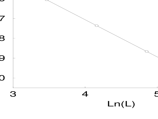
Figure 2: Leading FSS of the First Lee–Yang Zeroes $h_{1}(L)$ for the $XY$–model at $\beta=1.11$.

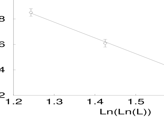
Figure 3: Corrections to FSS of the First Lee–Yang Zeroes for the $XY$–model at $\beta=1.11$.

We begin our analysis with the first Lee–Yang zeroes at the preliminary critical coupling estimate $\beta_{\rm{RW}}\simeq 1.11$. In Fig. 2 we plot the logarithm of the position of the first Lee–Yang zero against the logarithm of the lattice size $L$, at $\beta=1.11$. In the absence of any corrections, the slope should give the leading power–law exponent $\lambda$. In fact at $\beta=1.11$ the slope is $\lambda_{\rm{eff}}=-1.8778(2)$. The deviation from the KT value of $-15/8=-1.875$ can be attributed to (a) the presence of logarithmic corrections and/or (b) the possibility that $\beta=1.11$ is not in fact the critical point. As a preliminary investigation of (a) we identify the correction exponent $r$ in (2.32), by plotting $\ln{(\theta_{1}L^{15/8})}$ against $\ln{(\ln{L})}$ in Fig. 3. A straight line is identified. Its slope is $-0.012(1)$ giving evidence for a non–zero value of $r$, albeit not in agreement with the renormalization group predictions of $-1/16=-0.0625$ from [5].

The above estimate $\beta_{\rm{RW}}\simeq 1.11$ for the critical coupling came from an analysis in which the possibility of the existence of logarithmic corrections was ignored. At this point, we must allow for the possibility of the true critical coupling $\beta_{c}$ being different than $\beta_{\rm{RW}}$. To systematically investigate the extent to which the above conclusions depend on the measurement of $\beta_{c}$, we now study the above FSS (fits for $\lambda_{\rm{eff}}$) and corrections to FSS (fits for $r$) as a function of the assumed critical beta.

In Fig. 4a we plot $\lambda_{\rm{eff}}$ coming from fits to the leading FSS behaviour as a function of $\beta$. Fig. 4b gives the corresponding $\chi^{2}$ per degree of freedom [$\chi^{2}/{\rm{dof}}$] for these fits. Not all fits yield an acceptable $\chi^{2}/{\rm{dof}}$. To be conservative, we take ‘acceptable’ to mean

$$\chi^{2}/{\rm{dof}}\quad{\rm{\raisebox{-3.22916pt}{ {\small\shortstack{$<$ \\ $\sim$}} }}}\quad 2\quad,$$ (3.46)

which corresponds to a minimum confidence level of 14%. For Fig. 4 we have acceptable values of $\chi^{2}/{\rm{dof}}$ only for $\beta$ $>$ $\sim$ $1.107$. The figure indicates that FSS sets in above this value. I.e., the system remains critical for $\beta$ $>$ $\sim$ $1.107$.

This range of critical $\beta$ values corresponds to $\lambda_{\rm{eff}}$ $<$ $\sim$ $-1.8761(2)$. This range of critical $\beta$ values does not include that for which the KT value of $-15/8=-1.875$ is recovered (Fig. 4 gives $\lambda_{\rm{eff}}\simeq-1.875$ at $\beta\simeq 1.105$ with $\chi^{2}/{\rm{dof}}\simeq 3.4$). Thus we can conclude that ignoring logarithmic corrections gives deviation from the KT value of $-15/8=-1.875$ for $\lambda$.

Next we investigate how our conclusions regarding the correction exponent $r$ depend on the critical coupling. Fig. 5 gives the results from fits to $r$ from (2.32) and the corresponding $\chi^{2}/{\rm{dof}}$. we see that acceptable values are possible only for $1.107$ $<$ $\sim$ $\beta_{c}$ $<$ $\sim$ $1.119$. The $r=0$ solution again corresponds to $\beta_{c}\simeq 1.105$ and $\chi^{2}/{\rm{dof}}\simeq 3.4$. Similary, we find that a fit with $r=-1/16$ would correspond to $\beta_{c}\simeq 1.138$ and $\chi^{2}/{\rm{dof}}\simeq 13$.

Therefore we have numerical evidence challenging the detailed quantitative predictions of Kosteritz and Thouless. In summary, the results of the analysis of the first Lee–Yang zeroes of the $XY$–model is that assuming the KT value $\eta=1/4$, we find non-zero logarithmic corrections to scaling and a corresponding estimate of the critical temperature:

$$r=-0.02(1)\,,\qquad\beta_{c}=1.113(6)\,.$$ (3.47)

KT Versus Power Law Scaling Scenario

The KT essential scaling scenario was called into question in [14] where numerical evidence in support of conventional power law scaling behaviour in the $Z(10)$ clock model was given. While this model is expected to be in the same universality class at the $XY$–model (same critical indices) it may have a different critical coupling $\beta_{c}$ hindering a comparison with our numerical results. However a recent paper by Kim [28] also claims to favour a convential as opposed to KT phase transition in the $XY$–model.

It is extremely difficult to distinguish between KT and power law scaling on the basis of numerical methods alone [20]. Power law scaling for the thermodynamic functions (with additive power law corrections) would lead to (2.28) being replaced by Josephson’s law

$$\alpha=2-\nu d\quad,$$ (3.48)

and the FSS of the zeroes (2.32) by

$$\theta_{1}(\beta_{c})=a_{1}L^{\lambda}\left(1+a_{2}L^{a_{3}}\right)\quad,$$ (3.49)

for some $a_{1}$, $a_{2}$ and $a_{3}$. If $\nu>1$ the singular part of the specific heat decreases with lattice size as in the KT case (2.30). Thus Josephson’s law may not be a numerically useful criterion for distinguishing between the two scaling scenarios.

The leading FSS of $\theta_{1}$ in (3.49) is the same as for the KT case (2.32) and ignoring corrections leads to the same conclusions regarding $\lambda_{\rm{eff}}$. However, as seen above, it is essential to include corrections to correctly identify $\beta_{c}$. Ignoring corrections would lead us to conclusions similar to [28]. The numerical analysis of [28] applies to $\xi$ and $\chi$. There, $\eta(\beta)$ is measured by fitting to the FSS formula $\chi_{L}\sim L^{2-\eta(\beta)}$ (ignoring multiplicative logarithmic corrections). Good fits ($\chi^{2}/{\rm{dof}}<0.5$) were reported for $\beta>1.105$. Using

$$\lambda=-2+\eta/2\quad,$$ (3.50)

the corresponding $\lambda_{\rm{eff}}$ can be found. These are listed and compared to our own results (when corrections are ignored) in Table 3. The agreement is impressive.

Table 3: Comparison of our results for $\lambda_{\rm{eff}}$ (ignoring multiplicative logarithmic corrections) to [27].

$T$	$\beta=1/T$	$\eta$ from [28]	$\lambda_{\rm{eff}}$ from [28]	Our $\lambda_{\rm{eff}}$	Our $\chi^{2}/{\rm{dof}}$
0.910	1.099	0.2600(10)	-1.8700(10)	-1.8712(2)	9.0
0.905	1.105	0.2520(05)	-1.8740(05)	-1.8750(2)	3.4
0.900	1.111	0.2450(05)	-1.8770(05)	-1.8778(2)	0.8
0.890	1.1236	0.2310(10)	-1.8840(10)	-1.8838(2)	0.2

In [28] the critical point is located by finding a coupling, $\beta_{\rm{P}}$, where $\chi_{L}\sim L^{2-\eta(\beta)}$ holds for $\eta=1/4$. The result is $1.105<\beta_{\rm{P}}<1.111$ with ‘most probably’ $\beta_{\rm{P}}=1.1062(6)$ ($T_{c}=0.9040(5)$). This compares well to our result $r=0$ (no corrections) at $\beta\simeq 1.105$. Using this as the critical coupling, [28] reports that fits to $\xi$ in (1.5) give an unacceptable $\chi^{2}/{\rm{dof}}$. In the light of our analysis this is hardly surprising. The system is still in fact in the high temperature phase and criticality has not been reached – $\beta_{\rm{P}}$ is not the true critical coupling.

Examination of power law scaling in [28] in the form of a four parameter fit to $\xi_{\infty}=At^{-\nu}(1+bt^{w})$ yields a reasonable $\chi^{2}/{\rm{dof}}$. We attempted a three parameter fit to (3.49) and found acceptable $\chi^{2}/{\rm{dof}}$ over a range of values for $\beta$ but believe this to be attributable to the fact that it is easy to make a three parameter fit to only 4 data points. So while we cannot logically exclude a power law scaling scenario on the basis of our numerical results neither can the (modified) KT scaling scenario be excluded on the basis of [28].

The lesson here is that it is essential to include consideration of logarithmic corrections to KT scaling in order not to be led to the wrong value of $\beta_{c}$ upon which conclusions are highly sensitive.

3.3.3 The Step Model

Scaling of Lowest Lee–Yang Zeroes

The analysis began with a rough search for the leading critical behaviour predicted by (2.32). An independent test was also made using the (less accurate) susceptibility data and (2.22). Both methods indicated critical behaviour setting in for $\beta$ $>$ $\sim$ $1.2$.

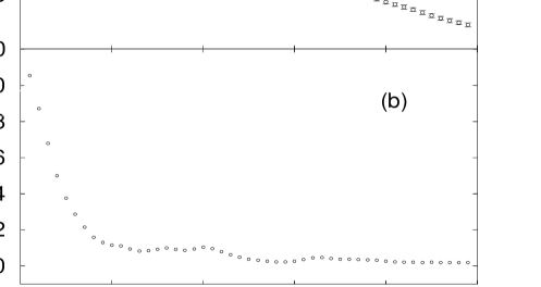
Figure 6: Test of the Expected Leading Critical Behaviour for the step model: (a) The effective exponent $\lambda_{\rm{eff}}^{\rm{step}}$ (slope of a straight line fit) and (b) the corresponding $\chi^{2}/{\rm{dof}}$ versus $\beta$.

In Fig. 6 we display the results for the effective exponent $\lambda_{\hbox{eff}}^{\rm{step}}$ as a function of $\beta$ together with the corresponding $\chi^{2}/{\rm{dof}}$. Acceptable fits are only found for $\beta_{c}^{\rm{step}}\raisebox{-3.22916pt}{ {\small\shortstack{$>$ \\ $\sim$}} }1.185$. We note that the corresponding values of $\lambda_{\hbox{eff}}^{\rm{step}}$ ($\raisebox{-3.22916pt}{ {\small\shortstack{$<$ \\ $\sim$}} }-1.8715(2)$) include that ($-15/8=-1.875$) corresponding to the KT prediction.

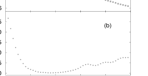
Figure 7: Logarithmic corrections for the step model: (a) the logarithmic correction exponent $r^{\rm{step}}$ to the Yang–Lee edge is shown as a function of the assumed critical coupling $\beta_{c}^{\rm{step}}$ and (b) the corresponding $\chi^{2}/{\rm{dof}}$.

Again, the evidence for critical behaviour is the existence of a range of acceptable chi-squared values for a linear fit. In view of the similarity of $\lambda_{\hbox{eff}}^{\rm{step}}$ to the expected KT value, we now proceed to test the further hypothesis that the step model is in fact in the same universality class as the $XY$–model. We assume the behaviour (2.32) with $\lambda^{\rm{step}}=-15/8$ and search for corrections in Fig. 7. We find acceptable fits for $1.195\leq\beta_{c}^{\rm{step}}\leq 1.295$ with $0.009\geq r\geq-0.034$.

The range of acceptable $r$ values includes that found earlier for the $XY$–model and that corresponding to no logarithmic corrections ($r=0$). Again, this range excludes the prediction $r=-1/16$ coming from the approximate renormalisation group treatment of the $XY$–model [5]. Thus we conclude that the present data are compatible with the step model being in the same universality class as the $XY$–model. We do not, however, exclude other possibilities.

In summary,

$$XY{\rm{-Model:}} 1.107\raisebox{-3.22916pt}{ {\small\shortstack{$<$ \\ $\sim$}} }\beta_{c}\raisebox{-3.22916pt}{ {\small\shortstack{$<$ \\ $\sim$}} }1.119\quad, -0.01\raisebox{-3.22916pt}{ {\small\shortstack{$>$ \\ $\sim$}} }r\raisebox{-3.22916pt}{ {\small\shortstack{$>$ \\ $\sim$}} }-0.03\quad,$$ (3.51)

$${\rm{Step~{}Model:}} 1.195\raisebox{-3.22916pt}{ {\small\shortstack{$<$ \\ $\sim$}} }\beta_{c}^{\rm{step}}\raisebox{-3.22916pt}{ {\small\shortstack{$<$ \\ $\sim$}} }1.295\,, 0.01\raisebox{-3.22916pt}{ {\small\shortstack{$>$ \\ $\sim$}} }r^{\rm{step}}\raisebox{-3.22916pt}{ {\small\shortstack{$>$ \\ $\sim$}} }-0.03\,.$$ (3.52)

3.3.4 Higher Order Corrections

We have shown that a FSS analysis ignoring multiplicative logarithmic corrections leads to deviation from the KT prediction $-15/8$ for $\lambda$ or, equivalently, $1/4$ for $\eta(\beta_{c})$. When multiplicative logarithmic corrections are taken into account the results are compatible with $\eta(\beta_{c})=1/4$ but, now, the leading logarithm exponent $r$ is not that given by KT.

In the same spirit, it is conceivable that numerical measurement of these leading logarithmic corrections may become compatible with the KT RG predictions ($r=-1/16$) if higher order corrections are accounted for.

Keeping higher order (additive) corrections in the RG treatment of the magnetic susceptibility modifies the right hand side of (2.12) by [9, 10]

$$\left\{1+O\left(\frac{\ln{\ln{\xi_{\infty}}}}{\ln{\xi_{\infty}}}\right)\right\}\quad.$$ (3.53)

The FSS behaviour of the Yang–Lee edge is now expected to be (from (2.25))

$$\theta_{1}(\beta_{c})=a_{1}L^{\lambda}(\ln{L})^{r}\left\{1+a_{2}\frac{\ln{\ln{L}}}{\ln{L}}\right\}\quad.$$ (3.54)

Unbiased four parameter fits are hampered by the convergence problems mentioned in section 1.1. However, if we again accept the leading scaling behaviour $\lambda=-15/8$, two parameter fits to $a_{1}$ and $a_{2}$ in (3.54) yield unacceptable $\chi^{2}/{\rm{dof}}$ if $r$ is $-1/16$ in both the $XY$– and step models. In fact, $\chi^{2}/{\rm{dof}}$ ranges from $13$ to $2$ as $\beta$ decreases from $1.14$ to $1.10$ in the $XY$–model and from $9$ to $2.5$ as $\beta$ decreases from $1.40$ to $1.17$ in the step model, indicating that such fits may become acceptable for very low $\beta$ in both cases. (Note that in the case of the $XY$–model such low $\beta$ is outside the range of $\beta_{c}$–measurements in table 1). On the other hand, if we fix $r=-0.02$ we find $\chi^{2}/{\rm{dof}}{\rm{\raisebox{-3.22916pt}{ {\small\shortstack{$<$ \\ $\sim$}} }}}2$ over the whole $\beta$–range in both models.

4 Analysis of Higher Index Zeroes

In the calculation leading to (2.25) we assumed that the low index zeroes have the same FSS behaviour. We now wish to (a) check that assumption, (b) redo the whole analysis for each index $j=2,\dots,10$ separately and (c) introduce a new concept we call ‘index scaling’ and apply it to these first ten zeroes. In fact we can determine up to fifteen zeroes for each lattice size. However the errors for the highest index zeroes become too large to allow reliable analysis.

4.1 Analyses of Individual Higher Index Zeroes

Table 4: The results of the $\lambda_{\rm{eff}}$–analysis for the $j$–index zeroes for the $XY$– and step models: The criterion (3.46) holds for each $j$ for $\beta$ above and $\lambda$ below the values listed.

	$XY$–Model		step Model
$j$	$\beta$	$\lambda_{\rm{eff}}$	$\beta$	$\lambda_{\rm{eff}}$
01	1.107	-1.8761(2)	1.185	-1.8715(2)
02	1.107	-1.8761(2)	1.185	-1.8716(2)
03	1.106	-1.8754(2)	1.180	-1.8716(2)
04	1.106	-1.8753(2)	1.185	-1.8717(2)
05	1.104	-1.8741(2)	1.190	-1.8725(2)
06	1.103	-1.8735(2)	1.200	-1.8739(2)
07	1.103	-1.8735(2)	1.215	-1.8757(2)
08	1.103	-1.8735(2)	1.215	-1.8757(2)
09	1.100	-1.8717(2)	1.195	-1.8735(2)
10	1.100	-1.8717(2)	1.185	-1.8722(2)

Table 5: The Results of the $r$–Analysis for the $j$–Index Zeroes for the $XY$– and step models: The criterion (3.46) holds for each $j$ for the following $\beta$ ranges and corresponding $r$ range.

	$XY$–Model		step Model
$j$	$\beta$	$r$	$\beta$	$r$
01	1.107–1.119	-0.005(1) – -0.030(1)	1.195–1.295	0.009(1) – -0.034(1)
02	1.106–1.120	-0.002(1) – -0.032(1)	1.195–1.295	0.009(1) – -0.034(1)
03	1.106–1.120	-0.002(1) – -0.031(1)	1.195–1.295	0.008(1) – -0.034(1)
04	1.105–1.119	0.001(1) – -0.029(1)	1.195–1.295	0.008(1) – -0.034(1)
05	1.104–1.117	0.004(1) – -0.024(1)	1.200–1.295	0.005(1) – -0.034(1)
06	1.104–1.116	0.004(1) – -0.022(1)	1.205–1.295	0.002(1) – -0.034(1)
07	1.104–1.116	0.004(1) – -0.022(1)	1.210–1.300	-0.001(1) – -0.035(1)
08	1.103–1.116	0.007(1) – -0.021(1)	1.210–1.300	0.001(1) – -0.035(1)
09	1.102–1.119	0.009(1) – -0.026(1)	1.200–1.310	0.004(1) – -0.038(1)
10	1.100–1.122	0.014(1) – -0.031(1)	1.190–1.350	0.009(1) – -0.047(1)

We repeat the analysis of (2.32) for each index separately for $j=2,\dots,10$ and for both the $XY$– and step models. The results of the analyses for $\lambda_{\rm{eff}}$ are sumarized in Table 4. For the $XY$–model the analysis applied to individual higher index zeroes ($j$ $>$ $\sim$ $4$) appears to accomodate the $RG$ result $\lambda=-1.875$. However higher index zeroes are less accurately determined than lower index ones and the $j=1$ results remain the most accurate.

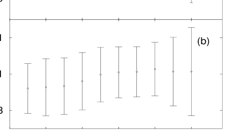
Figure 8: Minimum and maximum acceptable (a) $\beta$ and (b) correction exponent $r$ from the $r$–analysis with criterion (3.46) for the $XY$–model.

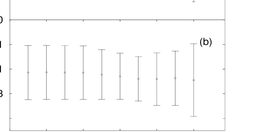
Figure 9: Minimum and maximum acceptable (a) $\beta$ and (b) correction exponent $r$ from the $r$–analysis with criterion (3.46) for the step model.

Accepting $\lambda=-1.875$ and looking for corrections from applications of the $r$–analysis to each index $j$ separately gives the results summarized in Table 5. Acceptable fits are obtained only in the $\beta$ range given and lead to the listed ranges for $r$. These $\beta$ and $r$ ranges are graphically represented in Fig. 8 (for the $XY$–model) and Fig. 9 (for the step model). Although in both models the higher index zeroes individually allow for $r=0$, at no stage (up to $j=10$) do we find results compatable with the RG result $-1/16=-0.0625$. So the higher index zeroes analysed individually yield the same information with decreasing accuracy as $j$ increases providing further strong evidence of the validity of our earlier conclusions.

Finally, analyses of higher order (additive) corrections for the individual higher index zeroes yield the same qualitative results as those presented in sec. 3.3.4.

4.2 Analysis of the Density of Zeroes (Index Scaling)

The last section demonstrates the success of FSS applied to each zero separately. We can now be confident that the lowest lying zeroes scale in the same way with lattice size $L$ and that this scaling behaviour is

$$\theta_{j}(\beta_{c})\sim L^{\lambda}(\ln{L})^{r}\quad.$$ (4.55)

In this paragraph we wish to report an attempt to combine the scaling behaviour of the various indexed zeroes.

The density of zeroes for the finite (binned) system is given in (2.6) as a sum over delta functions,

$$g_{L}(\beta,\theta)=L^{-d}\sum_{j=1}^{N}\delta(\theta-\theta_{j}(\beta,L))\quad,$$ (4.56)

where $N$ is the total number of zeroes. The corresponding cumulative density function $G$ is a step function with

$$G_{L}(\beta,\theta)=\frac{j}{N}\quad\quad\quad{\rm{if}}\quad\theta\in(\theta_{j},\theta_{j+1})\quad.$$ (4.57)

This function can be smeared by replacing the delta functions of (4.56) by Gaussians

$$g_{L}(\beta,\theta)=\frac{1}{N}\sum_{j=1}^{N}{\frac{1}{\sqrt{2\pi}\sigma_{j}(L)}e^{-\frac{1}{2}\left(\frac{\theta-\theta_{j}(\beta,L)}{\sigma_{j}(L)}\right)^{2}}}\quad,$$ (4.58)

where $\sigma_{j}(L)$ is some appropriate quantity giving the spread of the Gaussian around the $j^{\rm{th}}$ zero. The cumulative density function is then a sum of error functions

$$G_{L}(\beta,\theta)=\frac{1}{2N}\sum_{j=1}^{N}{\left(1+{\rm{erf}}{\left(\frac{\theta-\theta_{j}}{\sqrt{2}\sigma_{j}}\right)}\right)}\quad.$$ (4.59)

If $\sigma_{j}(L)$ is small enough then

$$G_{L}(\beta,\theta_{j})=\frac{2j-1}{2N}\quad.$$ (4.60)

In the thermodynamic limit (2.10) gives

$$G_{\infty}(\beta,\theta)\sim\xi_{\infty}^{-d}\Phi\left(\frac{\theta}{\theta_{c}(\beta)}\right)\quad.$$ (4.61)

The corresponding FSS formula is

$$G_{L}(\beta_{c},\theta)\propto L^{-d}\Phi\left(\frac{\theta}{\theta_{1}(\beta_{c})}\right)\quad.$$ (4.62)

Comparing with (4.60) and using $N\propto L^{d}$,

$$\frac{\theta_{j}}{\theta_{1}}=\Phi^{-1}\left(\Phi(1)(2j-1)\right)\quad.$$ (4.63)

The density of zeroes in the thermodynamic limit is

$$g_{\infty}(\beta,\theta)=\frac{dG_{\infty}(\beta,\theta)}{d\theta}=\xi_{\infty}^{-d}\theta_{c}^{-1}\Phi^{\prime}\left(\frac{\theta}{\theta_{c}(\beta)}\right)\quad.$$ (4.64)

In a numerical high temperature and high field study, Kortman and Griffiths showed that, for Ising models in the high temperature phase, this density exhibits power law behaviour as a function of the distance of $\theta$ away from the edge [49],

$$\Phi^{\prime}\left(\frac{\theta}{\theta_{c}(\beta)}\right)\sim\left|1-\frac{\theta}{\theta_{c}(\beta)}\right|^{\sigma}\quad.$$ (4.65)

At $\beta=\beta_{c}$, $\sigma=1/\delta$ where $\delta$ is the usual magnetization index. This index governs the response of the magnetization to the presence of a weak external magnetic field,

$$M\sim h^{\frac{1}{\delta}}\quad.$$ (4.66)

One therefore is led to expect

$$\Phi(x)\sim(1-x)^{\frac{\delta+1}{\delta}}\quad,$$ (4.67)

or,

$$\Phi^{-1}(y)-1\sim y^{\frac{\delta}{\delta+1}}\quad.$$ (4.68)

There are additive higher order corrections to formulae (4.61)–(4.66). Now, (4.63) gives

$$\frac{\theta_{j}}{\theta_{1}}=c_{1}+c_{2}(2j-1)^{\frac{\delta}{\delta+1}}\quad,$$ (4.69)

for some $c_{1}$ and $c_{2}$ which incorporate the higher order corrections. Using the standard scaling relation

$$\delta=\frac{d+2-\eta}{d-2+\eta}\quad,$$ (4.70)

we can express the leading behaviour in terms of $\lambda$

$$\frac{\theta_{j}}{\theta_{1}}=c_{1}+c_{2}(2j-1)^{-\frac{\lambda}{d}}\quad.$$ (4.71)

Again, one expects there to be additive volume dependent corrections to this formula.

Nonetheless, to leading order the $L$–dependence drops out of the ratio of the $j^{\rm{th}}$ to $1^{\rm{st}}$ zeroes. This opens up the possibility of a new type of scaling technique – the use of the dependency of this ratio on the index $j$ to find critical indices. If successful, this method could be applied in parallel to traditional FSS. The advantage would be that one doesn’t need enormous lattices to eliminate finite–size effects, nor does one need a large range of lattice sizes to exploit FSS. In cases where only one lattice size is available, index scaling may, in principle, still yield a result.

We can check the form (4.69) in one dimension. From the exact solution to the one dimensional Ising model with periodic boundary conditions, the Lee–Yang zeroes are given by [31]

$$\cos{(2\theta_{j})}=-u^{2}+(1-u^{2})\cos{\left(\frac{2j-1}{L}\pi\right)}\quad,$$ (4.72)

where $u=\exp{(-2\beta)}$. In one dimension the critical point is at zero temperature or $u_{c}=0$. Then the LY zeroes are at

$$\theta_{j}(\beta_{c})=\pm\frac{2j-1}{2L}\pi\quad.$$ (4.73)

Then,

$$\frac{\theta_{j}}{\theta_{1}}=2j-1\quad,$$ (4.74)

which is of the form (4.69) with $\delta=\infty$, the correct value for $\delta$ in one dimension. There is no exact solution to the Ising model in the presence of an external field in two or more dimensions.

The $XY$–Model

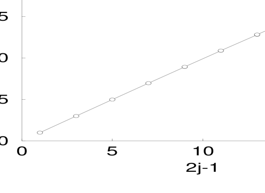
Figure 10: Index scaling in the $XY$–model at $\beta_{c}=1.115$. The errors are smaller than the symbols. Each symbol is in fact an overlap of four data points coming from the four lattice sizes demonstrating excellent $L$–collapse.

In Fig. 10 we test (4.71) for the two dimensional $XY$–model at $\beta_{c}=1.115$. The plot involves ten LY zeroes for each of the four lattice sizes – forty data points in all. As expected, no $L$–dependence is visible. Fitting to

$$\frac{\theta_{j}}{\theta_{1}}=c_{1}+c_{2}(2j-1)^{c_{3}}$$ (4.75)

gives, however, $c_{3}=0.9827(3)$, 5% away from the expected value $-\lambda/d=0.9375$ and a rather poor $\chi^{2}/{\rm{dof}}$ ($8.7$). The line in Fig. 10 is this best fit to (4.75).

In an early paper on the scaling of partition function zeroes [56] it was suggested that the scaling variable is in fact $j/L^{d}$. When we plot $h_{j}(L)$ against $j/L^{d}$ we find the data does not collapse onto a smooth curve. A later paper showed that this dependency only holds for high index zeroes [69]. Indeed our result

$$\theta_{j}=\theta_{j}\left(\frac{2j-1}{L^{d}}\right)$$ (4.76)

asymptotically approaches that of [56] at high $j$. However, the poor $\chi^{2}/{\rm{dof}}$ for the fit to the form (4.75) indicates that while it might be nearer the truth than [56], (4.76) is also not the full story .

Table 6: The Results of the index scaling Analysis small ranges of $j$.

$j$	$c_{3}$
2-5	0.991(1)
3-6	0.986(1)
4-7	0.981(1)
5-8	0.977(1)
6-9	0.973(1)
7-10	0.969(2)

To see how $c_{3}$ depends on the $j$–indices used, we make fits to (4.75) for $j=2-5$, $3-6$ and so on to $7-10$. We have a three parameter fit to $4\times 4=16$ data points in each case. The fits are now of good quality ($\chi^{2}/{\rm{dof}<1}$) and the results for $c_{3}$ are summarised in Table 6. The j–dependence indicates that (4.75) can only be true asymptotically and encourages further investigation into the the full scaling form. A similar picture is found for the step model.

5 Conclusions

We have presented a very general (model independent) theoretical method to test the self–consistency of the scaling behaviour of odd and even thermodynamic functions. Application of this method to the KT scaling predictions for the two dimensional $XY$–model reveals that multiplicative logarithmic corrections cannot be ignored. In the case of specific heat these logarithmic corrections were identified analytically. The corrections corresponding to the magnetic susceptibility were identified numerically from the scaling behaviour of the lowest Lee–Yang zeroes.

The theoretical and numerical techniques we have developed are fully independent of the physics of the phase transition. The conventional picture is that the $XY$–model phase transition is driven by a vortex binding mechanism [4, 5]. This is in contrast to the customary picture of the step model [32, 33, 34, 35, 36, 37, 39]. Here, while the configuration space is the same as that of the $XY$–model, vortex formation is not believed to be energetically favourable given the discontinuous nature of the interaction function. If the $XY$–model phase transition is truely driven by a vortex interaction mechanism and if a phase transition exists at all in the step model then, barring a remarkable coincidence, they are expected to belong to different universality classes (different scaling behaviour).

Application of our numerical techniques to the two dimensional step model reveals the critical parameters (including logarithmic corrections) to be compatable with those of the $XY$–model. This is a strong indicaton that both models do in fact belong to the same universality class. This conclusion is reinforced by analysis of higher index zeroes.

This result raises questions on how the vortex binding scenario can be the driving mechanism for the phase transition in the $XY$–model. Furthermore, the multiplicative logarithmic corrections identified numerically by the analysis of up to the first ten Lee–Yang zeroes are not in agreement with the renormalization group predictions of Kosterlitz and Thouless.

Note

Since the preprint version of this paper first appeared, other authors have reanalysed their data to look for logarithmic corrections in the two dimensional $XY$–model. In particular, Janke [71] has applied FSS to the Villain version and found $r=-0.027(1)$ in agreement with our result. High temperature measurements [71] give $r=+0.0560(17)$, close to Patrascioiu and Seiler’s result $r=+0.077(46)$ [72] and $r=+0.042(5)$ to $+0.05(2)$ from Campostrini et al. [73].

We wish to thank W. Janke, E. Klepfish and C.B. Lang for stimulating discussions.

Figure 1: The Roomany–Wyld beta function approximants for (a) the $XY$–model and (b) the step model. The symbols $\Box$, $\circ$, $\times$ and $\bullet$

are in order of increasing lattice size.

Figure 4: Test of the Expected Leading Critical Behaviour for the $XY$–model: (a) The effective exponent $\lambda_{\rm{eff}}$ (slope of a straight line fit) and (b) the corresponding $\chi^{2}/{\rm{dof}}$ versus $\beta$.

Figure 5: Logarithmic corrections for the $XY$–model: (a) the logarithmic correction exponent $r$ to the Yang–Lee edge is shown as a function of the assumed critical coupling $\beta_{c}$ and (b) the corresponding $\chi^{2}/{\rm{dof}}$.

References

- [1]
- [2] N.D. Mermin and H. Wagner, Phys. Rev. Lett. 22 (1966) 1133.
- [3] S. Coleman in New Phenomena in Subnuclear Physics, Proc. 13th International School of Subnuclear Physics, Erice, ed. A. Zichichi (Plenum Press, NY, 1977) 297.
- [4] V. Berezinskii, Zh. Eksp. Teor. Fiz. 59 (1970) 907 [Sov. Phys., JETP 32 (1971) 493]; Zh. Eksp. Teor. Fiz. 61 (1971) 1144 [Sov. Phys., JETP 34 (1971) 610].
- [5] J. Kosterlitz and D. Thouless, J. Phys. C6 (1973) 1181; J. Kosterlitz, J. Phys. C7 (1974) 1046.
- [6] R.J. Baxter, ‘Exactly Solved Models in Statistical Physics’, Academic Press, (1982).
- [7] J.V. José, L. Kadanoff, S. Kirkpatrick and D.R. Nelson, Phys. Rev. B 16 (1977) 1217.
- [8] P.B. Wiegmann, J. Phys. C 11 (1978) 1583.
- [9] D.J. Amit, Y.Y. Goldschmidt and G. Grinstein, J. Phys. A 13 (1980) 585.
- [10] A.B. Zisook and L.P. Kadanoff, J. Phys. A 13 (1980) L379; L.P. Kadanoff and A.B. Zisook, Nucl. Phys. B 180[FS2] (1981) 61.
- [11] M. Hasenbusch, M. Marcu and K. Pinn, Physica A 208 (1994) 124.
- [12] R. Gupta, J. De Lapp, G. Batrouni, G.C. Fox, C.F. Baillie and J. Apostolakis, Phys. Rev. Lett. 61 (1988) 1996.
- [13] J.F. Fernández, M.F. Ferreira and J. Stankiewicz, Phys. Rev. B 34 (1986) 292.
- [14] E. Seiler, I.O. Stamatescu, A. Patrascioiu and V. Linke, Nucl. Phys. B 305 [FS23] (1988) 623.
- [15] U. Wolff, Phys. Rev. Lett. 62 (1989) 361; Nucl. Phys. B 322 (1989) 759.
- [16] L. Biferale and R. Petronzio, Nucl. Phys. B 328 [FS28] (1989) 677.
- [17] P. Butera, m. Comi and G. Marchesini, Phys. Rev. B 33 (1986) 4725; P. Butera, m. Comi and G. Marchesini, Phys. Rev. B 40 (1989) 534.
- [18] M. Ferer and Z. Mo, Phys. Rev. B 42, (1990) 10769.
- [19] A. Hulsebos, J. Smit, J.C. Vink, Nucl. Phys. B 356 (1991) 775.
- [20] R.G. Edwards, J. Goodman and A.D. Sokal, Nucl. Phys. B 354 (1991) 289.
- [21] R. Gupta and C.F. Baille, Nucl. Phys. B (Proc. Suppl.) 20 (1991) 669; Phys. Rev. B 45 (1992) 2883.
- [22] P. Butera and M. Comi, Phys. Rev. B 47 (1993) 11969.
- [23] W. Janke and K. Nather, Phys. Lett. A, 157, (1991) 11; Phys. Rev. B 48 (1993) 7419.
- [24] S.M. Catterall, J.B. Kogut and R.L. Renken, Nucl. Phys. B 408 (1993) 427.
- [25] P. Butera and M. Comi, Phys. Rev. B 50, (1994) 3052.
- [26] N. Schultka and E. Manousakis, Phys. Rev. B 49 (1994) 12071.
- [27] P. Olsson, Phys. Rev. B 52 (1995) 4511; ibid. 4526.
- [28] J.-K. Kim UCLA preprint 1995 (hep-lat/9502002), to appear in Phys. Lett. A.
- [29] M. Campostrini, A. Pelissetto, P. Rossi and E. Vicari, Nucl. Phys. B (Proc. Suppl.), 47 (1996) 755.
- [30] R. Kenna and A.C. Irving, Nucl. Phys. B (Proc. Suppl.) 42 (1995) 773; Phys. Lett. B 351 (1995) 273.
- [31] C. N. Yang and T. D. Lee, Phys. Rev. 87 (1952) 404; ibid. 410.
- [32] A.J. Guttmann, G.S. Joyce and C. J. Thompson, Phys. Lett. A 38 (1972) 297.
- [33] A.J. Guttmann and G.S. Joyce, J. Phys. C 6 (1973) 2691.
- [34] I-H. Lee and R.E. Shrock, Phys. Rev. B 36 (1987) 3712.
- [35] I-H. Lee and R.E. Shrock, J. Phys. A 21 (1988) 2111.
- [36] A. Nymeyer and A.C. Irving, J. Phys. A 19 (1986) 1745.
- [37] E. Sánchez-Velasco and P. Wills, Phys. Rev. B 37 (1988) 406.
- [38] A. Patrascioiu and E. Seiler, J. Stat. Phys. 69 (1992) 573.
- [39] A.J. Guttmann and A. Nymeyer, J. Phys. A 11 (1978) 1131.
- [40] A. Patrascioiu and E. Seiler, Phys. rev. Lett. 60 (1988) 875.
- [41] J. Zittartz, Z. Phys. B 23, (1976) 55, 63.
- [42] A. Luther and D.J. Scalpino, Phys. Rev. B 16, (1977) 1356.
- [43] F. Fucito and S. Solomon, Phys. Lett. B134, (1984) 235.
- [44] A. Patrascioiu and E. Seiler, Phys. Rev. Lett. 74 (1995) 1920; Nucl. Phys. B (Proc. Suppl.) 42 (1995) 826.
- [45] A.C. Irving and R. Kenna, Phys. Rev. B 53 (1996), 11568.
- [46] F. Dunlop and C.M. Newman, Commun. Math. Phys. 44 (1975) 223.
- [47] M. Salmhofer, Nucl. Phys. B (Proc. Suppl.) 30 (1993) 81; Helv. Phys. Acta 67 (1994) 257.
- [48] G. Gallavotti, S. Miracle–Sole and D.W. Robinson, Phys. Lett. 25A (1967) 493; Commun. Math. Phys. 10 (1968) 311.
- [49] P. Kortmann and R. Griffiths, Phys. Rev. Lett. 27 (1971) 1439.
- [50] R. Abe, Prog. Theor. Phys. 37, 1070 (1967) 1070; Prog. Theor. Phys. 38, 72; ibid. 322; ibid. (1967) 568.
- [51] M. Suzuki, Prog. Theor. Phys. 38, (1967) 289; ibid. 1225; ibid. 1243; Prog. Theor. Phys. 39, (1968) 349.
- [52] R. Kenna and C.B. Lang, Phys. Rev. E49 (1994) 5012.
- [53] M.E. Fisher and A.E. Ferdinand, Phys. Rev. Lett. 19 (1967) 169; M.E. Fisher and M.N. Barber, Phys. Rev. Lett. 28 (1972) 1516; M.E. Fisher, in Critical Phenomena, Proc. 51th Enrico Fermi Summer School, Varena, ed. M.S. Green (Academic Press, NY, 1971).
- [54] R. Kenna and C.B. Lang, Phys. Lett. B 264 (1991) 396; Nucl. Phys. B (Proc. Suppl.) 30 (1993) 697; Nucl. Phys. B 393 (1993) 461; Err. ibid. B 411 (1994) 340.
- [55] J.M. Luck, J. Phys. A15 (1982) L169.
- [56] C. Itzykson, R.B. Pearson, and J.B. Zuber, Nucl. Phys. B 220, 415 (1983); C. Itzykson and J.M. Luck, Progress in Physics, Critical Phenomena (1983 Brasov Conference) Birkhäuser, Boston Inc. 11, (1985) 45.
- [57] M. N. Barber, in Phase Transitions and Critical Phenomena, edited by C. Domb and J. Lebowitz (Academic Press, New York, 1983), Vol. VIII.
- [58] C. Allton and C. Hamer, J. Phys. A 21 (1988) 2417.
- [59] R.H. Swendsen and J.-S. Wang, Phys. Rev. Lett. 58 (1987) 86; J.-S. Wang and R.H. Swendsen, Physica A 167 (1990) 565.
- [60] E. Marinari, Nucl. Phys. B 235[FS 11] (1984) 123.
- [61] A.M. Ferrenberg and R.H. Swendsen, Phys. Rev. Lett. 61 (1988) 2635; Computers in Physics, Sep/Oct 1989.
- [62] P.B. Bowen et al., Phys. Rev. B 40 (1989) 7439.
- [63] K. Kajantie, L. Kärkkäinen and K. Rummukainen, Nucl. Phys. B 357 (1991) 693.
- [64] K. Binder and D. Stauffer, in Applications of the Monte Carlo Method in Statistical Physics, edited by K. Binder (Springer, Berlin, 1987), 1.
- [65] M.P. Nightingale, Physica 83A (1976) 561.
- [66] H. Roomany and H.W. Wyld, Phys. Rev. D21 (1980) 3341.
- [67] C.G. Callan, Jr., Phys. Rev. D 2 (1970) 1541; K. symanzik, Commun. Math. Phys. 18 (1970) 227.
- [68] A.C. Irving and C. Hamer, Nucl. Phys. B 230[FS10] (1984) 361; C. Hamer and A.C. Irving, J. Phys. A 17 (1984) 1649.
- [69] M. L. Glasser, V. Privman, and L. S. Schulman, J. Stat. Phys. 45, (1986) 451; Phys. Rev. B 35, (1987) 1841.
- [70] K.–C. Lee, Phys. Rev. Lett. 73, 2801 (1994).
- [71] W. Janke, preprint KOMA-96-17 (hep-lat/9609045), to appear in Phys. Rev. B.
- [72] A. Patrascioiu and E. Seiler, Phys. Rev. B. 54 (1996) 7177.
- [73] M. Campostrini, A. Pelissetto, P. Rossi and E. Vicari, Phys. Rev. B. 54 (1996) 7301.