A microscopic semiclassical confining field equation for $U(1)$ lattice gauge theory in 2+1 dimensions

Abstract

We present a semiclassical nonlinear field equation for the confining field in 2+1–dimensional $U(1)$ lattice gauge theory (compact QED). The equation is derived directly from the underlying microscopic quantum Hamiltonian by means of truncation. Its nonlinearities express the dynamic creation of magnetic monopole currents leading to the confinement of the electric field between two static electric charges. We solve the equation numerically and show that it can be interpreted as a London relation in a dual superconductor. (UFTP preprint 405/1996)

1 Introduction

In the last few years, several studies of confinement in lattice gauge theories have succeded in observing not only the confinement potential [1, 2], but also the formation of flux tubes between two static charges [3, 4]. The most promising mechanism for this effect is the dual superconductor hypothesis [5, 6, 7] which assumes that the electric field is confined by magnetic monopole currents forming the walls of the flux tube, just like superconducting electric currents confine the magnetic field in an ordinary superconductor. The monopoles are presumed to originate dynamically from the periodicity of the Hamiltonian as tunneling effects between neighboring minima [8, 9]. Abelian monopoles occur naturally in $U(1)$ lattice gauge theory (compact QED). As $U(1)$ is a subgroup of $SU(2)$ and $SU(3)$, so-called “Abelian” monopoles (monopoles in the maximally Abelian projection) [10] may also play a role in the QCD mechanism of confinement. The dynamic creation of magnetic monopoles and their description by a London relation has been observed in several studies [11, 12, 13, 14, 15] based on DeGrand and Toussaint’s identification prescription [11] for monopoles.

Recently, Zach et. al. [17] demonstrated that confinement of the electric field in $U(1)$ lattice gauge theory can be effectively described by the Maxwell-London equations of a dual superconductor. This model has only a single parameter, the London penetration length. It is, however, phenomenological in the sense that it is not derived from the underlying microscopical lattice system.

Most studies have employed Wilson’s Euclidean picture of lattice gauge theory [16], simulating it as a statistical system using Monte Carlo methods. While this offers easy access to the confining potential (string tension) by measuring the expectation value of a Wilson loop, and to the monopole density by means of the DeGrand-Toussaint prescription, measurements of the fields involves a more complex correlation function (basically between a loop and a plaquette) and thus more statistical fluctuations.

An alternative approach is to make use of the Kogut-Susskind Hamiltonian formulation [18], considering the theory as a quantum system with many degrees of freedom and applying methods from many-body theory as developed in e.g. computational chemistry or nuclear physics [19, 20, 21, 22, 23, 24]. In particular, the Hamiltonian formulation provides more easily for a semiclassical static solution than the Euclidean version.

In the following, we perform an ab initio derivation of a semiclassical field equation in $2+1$ dimensions that incorporates the prime feature of the gauge group $U(1)$—the periodicity of the action that leads to the dynamic creation of effective monopole currents. The resulting nonlinear field equation exhibits confinement of the electric field caused by magnetic monopole currents. It is microscopic in the sense that it is formulated in terms of the plaquette variables (i.e. the vortex potential of the electric field) and does not make use of phenomenologically introduced monopole fields.

We first review the formulation of classical electrodynamics on the lattice. After introducing the Kogut-Susskind Hamiltonian, we move to the plaquette representation (which only exists without constraints in 2+1 dimensions) and then perform a truncation of the Hilbert space to obtain a governing equation for plaquette wavefunctions. By studying single-plaquette solutions, we are led to an effective field equation in terms of the plaquette variables. Its linearized form is the London relation. The numerical solution shows confinement of the electric field. We discuss the consequences of this for the confinement of charges in lattice gauge theories.

2 Derivation of the effective field equations

2.1 Classical electrodynamics on the lattice

We are interested in the distribution of the electric field $E_{l}$ on the links $l$ of a 2-dimensional rectangular lattice in the presence of static charges. In the continuum, the electric field is determined by two conditions

$$\vec{\nabla}\cdot\vec{E}(\vec{r})=\rho_{e}(\vec{r})\quad,$$ (1)

$$\vec{\nabla}\times\vec{E}(\vec{r})=0\quad.$$ (2)

The first is Gauss’ law, expressing that the electric charge density is the source of the electric field, the second Stokes’ law that there are no closed lines of force (when we consider the static case without currents). These two equations determine the electric field completely. If the field exhibits confinement, one or both of them have to be modified. As the first equation is linked to gauge invariance of the theory (which is not violated), the only possible modification is to replace the zero on the right-hand side of the curl equation by a quantity $-J$, interpreted as the density of magnetic monopole currents.

On the lattice, the electric field is represented by its flux $E_{l}$ along the directed links $l$. Gauss’ law then becomes a condition on the link fields $E_{l}$ joined at a site $s$

$$\sum_{l}\epsilon_{s,l}E_{l}=\rho_{l}$$ (3)

where $\epsilon_{s,l}$ is $+1$ if the link $l$ leads away from site $s$, $-1$ if it leads to site $s$, and zero otherwise. In other words, the difference of inbound and outbound flux at any site equals the charge at this site.

Stokes’ law turns into a condition on each plaquette $p$,

$$\sum_{l}\epsilon_{p,l}E_{l}=-J_{p}$$ (4)

where $\epsilon_{p,l}$ is $+1$ or $-1$ if the directed link $l$ counts positively or negatively, resp., when going counter-clockwise around the plaquette. This condition states that the electric flux around a plaquette is generated by magnetic monopole currents.

2.2 Quantum electrodynamics on the lattice

In quantum field theory, the electromagnetic field is governed by the Kogut-Susskind Hamiltonian [18] for the gauge group $U(1)$:

$$H=-\frac{1}{2}\sum_{l\in\mbox{\scriptsize links}}\frac{\partial^{2}}{\partial^{2}\Theta_{l}}+\lambda\sum_{p\in\mbox{\scriptsize plaquettes}}\left(1-\mbox{Re}\,e^{i\Theta_{p}}\right)\quad,$$ (5)

where $\lambda=1/g^{4}$, $\Theta_{l}$ is the group parameter associated with the link $l$, and $\Theta_{p}$ the counter-clockwise sum of the link parameters around the plaquette $p$,

$$\Theta_{p}=\sum_{l}\epsilon_{p,l}\Theta_{l}\quad.$$ (6)

The Hamiltonian operates on a Hilbert space spanned by basis states

$$\mbox{$|\Theta\rangle$}=\prod_{l\in\mbox{\scriptsize links}}\mbox{$|\Theta_{l}\rangle$},\qquad-\pi\leq\Theta_{l}<\pi\quad.$$ (7)

The first (kinetic) term in eq. (5) is associated with the electric field, the second (potential) term with the magnetic field. Without the nonlinearity introduced by the higher-order terms of the cosine in the magnetic field term, this Hamiltonian would describe the motion of (nonrelativistic) particles in a harmonic potential (noncompact QED). In compact QED, the harmonic potential is replaced by a periodic potential that can be effectively described, as we shall see, by the dynamic creation of monopole currents.

As we are interested in the electric field, it is advantageous to switch to eigenstates of the momentum operator

$$\hat{n}_{l}=-i\frac{\partial}{\partial\Theta_{l}}$$ (8)

given by

$$\mbox{$\langle\Theta_{l}|n_{l}\rangle$}=e^{in_{l}\Theta_{l}}\quad.$$ (9)

The Hilbert space will then be spanned by basis states $|n\rangle$ whose label $n$ stands for a set of integer numbers $n_{l}$, one for each link $l$:

$$\mbox{$|n\rangle$}=\prod_{l\in\mbox{\scriptsize links}}\mbox{$|n_{l}\rangle$},\quad n_{l}\in{\bf Z}\quad.$$ (10)

In this representation, the Hamiltonian can be written

$$H=\frac{1}{2}\sum_{l\in\mbox{\scriptsize links}}\hat{n}^{2}_{l}+\lambda\sum_{p\in\mbox{\scriptsize plaquettes}}\left(1-\frac{1}{2}\hat{U}_{p}-\frac{1}{2}\hat{U}^{+}_{p}\right)\quad,$$ (11)

where $n$ represents the momentum operator (8) with the matrix element

$$\mbox{$\langle n^{\prime}|\hat{n}|n\rangle$}=n\,\delta_{n,n^{\prime}}\quad,$$ (12)

and the group element operator $\hat{U}_{p}$

$$\hat{U}_{p}=e^{i\Theta_{p}}$$ (13)

with the matrix elements

$$\mbox{$\langle n^{\prime}|\hat{U}_{p}|n\rangle$}=\delta_{n^{\prime},n+p}\quad,\qquad\mbox{$\langle n^{\prime}|\hat{U}^{+}_{p}|n\rangle$}=\delta_{n^{\prime},n-p}\quad,$$ (14)

where $n^{\prime}-p$ represents the configuration $n^{\prime}$ with all links in the plaquette $p$ raised or lowered by one unit according to whether they count positively or negatively when traversing the links of the plaquette counter-clockwise.

Note that the periodicity of the action has now transformed into the discretization of the dynamic variable $n$. This is the only nonlinearity in this equation.

The Hamiltonian (11) commutes with the operators

$$\hat{G}_{s}=\sum_{l\in\mbox{\scriptsize links}}\epsilon_{s,l}\hat{n}_{l},\qquad s\in\mbox{sites}$$ (15)

that generate gauge transformations at the lattice sites $s$. In the electric field representation, these operators are diagonal and their eigenvalues give the total electric field flux out of the sites $s$. By means of Gauss’ law (3), they are associated with static charges sitting at the lattice sites $s$. The eigenstates of the Hamiltonian separate into different sectors, each associated with a certain distribution of integer charges over the lattice sites. We are especially interested in the string sector with two opposite charges a certain distance away from each other.

In the strong-coupling limit $\lambda\to 0$, the Hamiltonian is dominated by the electric term. The lowest eigenstate in the string sector is the shortest path of raised links connecting the two charges. As the magnetic contribution is switched on by raising $\lambda$, perturbations are created from the original ground state by the action of the plaquette raising and lowering operators $U_{p}^{+}$ and $U_{p}$.

2.3 Plaquette representation

In two dimensions, self-duality of the lattice allows us to introduce new variables $m_{p}$ associated with plaquettes $p$ to replace the link variables $n_{l}$ by the relation

$$n_{l}=\sum_{p}\epsilon_{p,l}m_{p}+N_{l}$$ (16)

As there are exactly two plaquettes $p$ for which $\epsilon_{p,l}$ is nonzero, namely the plaquettes to the left ($\epsilon_{p,l}=1$) and to the right ($\epsilon_{p,l}=-1$) of the link $l$, (16) expresses each link as the difference of the two adjacent plaquettes. The corresponding continuum relation is

$$\vec{E}=\nabla\times\vec{m}+\vec{N}$$ (17)

where the vector field $\vec{m}$ is in the $z$-direction such that $\vec{E}$ is in the $x$-$y$-plane. Thus $\vec{m}$ is the vortex potential of the electric field. Gauss’ law is automatically satisfied

$$\vec{\nabla}\cdot\vec{E}=\vec{\nabla}\cdot\vec{N}=\rho_{e}$$ (18)

given an appropriate choice of $\vec{N}$ as a representative for the sector of the theory, e.g. a Dirac string for the two-charge sector. There is a residual gauge invariance under global shifts of the $m_{p}$.

The original Hilbert space is represented by the direct product of the set of all plaquette variable configurations $m_{p}$ and one configuration $N_{l}$ representative for each sector of the theory. It thus allows us to focus our attention on one sector by fixing $N_{l}$ while admitting all configurations $m_{p}$.

Turning first to the classical equations (3) and (4), we note that, while Gauss’ law is automatically satisfied, Stokes’ law becomes

$$4m_{p}-\sum_{(pp^{\prime})}m_{p^{\prime}}+N_{p}\equiv-\Delta_{L}m_{p}+N_{p}=-J_{p}$$ (19)

where the sum runs over all neighbors $p^{\prime}$ of the plaquette $p$, $\Delta_{L}$ is the lattice Laplace operator on an unit lattice, and $N_{p}$ is defined as the lattice curl of $N_{l}$

$$N_{p}=\sum_{l}\epsilon_{p,l}N_{l}\quad.$$ (20)

In particular, if $N_{l}$ is a string connecting two static charges, $N_{p}$ is $+1$ on the plaquettes just above the string and $-1$ just below the string.

The quantum Hamiltonian in the plaquette representation reads

$$H=2\sum_{p}\hat{m}_{p}^{2}-\sum_{(pp^{\prime})}\hat{m}_{p}\hat{m}_{p^{\prime}}+\frac{1}{2}\sum_{l}N_{l}^{2}+\sum_{p}\hat{m}_{p}N_{p}+\lambda\sum_{p}\left(1-\frac{1}{2}\hat{U}_{p}-\frac{1}{2}\hat{U}^{+}_{p}\right)$$ (21)

where $(pp^{\prime})$ sums over neighboring plaquettes $p^{\prime}$. We note that, while the diagonal (potential) part of (21) is quadratic and thus amenable to a Gaussian’ solution, the operators $U_{p}$ are highly nonlinear as they implicitly contain higher powers of the derivative operator. This, of course, is an expression of the fact that $m$ is confined to integer values which, in turn, results from the periodicity of the original $U(1)$ action and will ultimately give rise to a modification of Stokes’ equation. We also note that this restriction is enforced by the definition of $\hat{U}_{p}$ alone so that we may consider $m$ a continuous variable.

2.4 Truncation

To solve the eigenvalue problem of eq. (21), we truncate the eigenvalue equation to states that are direct products of single-plaquette states,

$$\mbox{$|\Psi\rangle$}=\prod_{p}\mbox{$|\psi_{p}\rangle$}\quad.$$ (22)

To find the governing equation for plaquette $q$, we project onto the state

$$\mbox{$|\Psi^{\prime}_{q}\rangle$}=\prod_{p\neq q}\mbox{$|\psi_{p}\rangle$}\quad.$$ (23)

This leads to the relation

$$\langle\Psi^{\prime}_{q}|H|\Psi\rangle = \left(\sum_{p\neq q}\mbox{$\langle\psi_{p}|H_{p}|\psi_{p}\rangle$}+\sum_{p\neq q}\sum_{p^{\prime}\neq q}\mbox{$\langle\psi_{p}\psi_{p^{\prime}}|H_{pp^{\prime}}|\psi_{p}\psi_{p^{\prime}}\rangle$}\right)\,\mbox{$|\psi_{q}\rangle$}$$ (24)

$$+ H_{q}\mbox{$|\psi_{q}\rangle$}+\sum_{p\neq q}\mbox{$\langle\psi_{p}|H_{qp}+H_{pq}|\psi_{p}\psi_{q}\rangle$}$$

$$= E\mbox{$|\psi_{q}\rangle$}$$

where the Hamiltonian was decomposed according to

$$H=\sum_{p}H_{p}+\sum_{pp^{\prime},p\neq p^{\prime}}H_{pp^{\prime}}+H_{0}$$ (25)

($H_{0}$ accounts for the constant part in the Hamiltonian). In this approximation, we find as the governing equation for the plaquette wavefunction $|\psi_{p}\rangle$

$$\left[2\hat{m}_{p}^{2}-\sum_{(pp^{\prime})}\hat{m}_{p}\langle m_{p^{\prime}}\rangle+\hat{m}_{p}N_{p}+\lambda\left(1-\frac{1}{2}\hat{U}_{p}-\frac{1}{2}\hat{U}^{+}_{p}\right)\right]\mbox{$|\psi_{p}\rangle$}=E_{p}\mbox{$|\psi_{p}\rangle$}\quad,$$ (26)

that is, a single-plaquette equation with the next-neighbor interaction replaced by a mean-field term. The single-plaquette energy $E_{p}$ is related to the total energy by

$$E_{p}=E-\sum_{q\neq p}\langle H_{q}\rangle-\sum_{q\neq p}\sum_{q^{\prime}\neq p}\langle H_{qq^{\prime}}\rangle-H_{0}\quad.$$ (27)

Summing over all $E_{p}$ would double-count the next-neighbor interactions. The correct ground-state energy is given by the expectation value of the Hamiltonian. However, since we have dropped all correlations between plaquettes, its value in this approximation cannot be trusted.

This approach can be extended to basis functions defined on a blocked lattice, as would be required for a renormalization group analysis.

2.5 Single-plaquette solutions

We rewrite the single-plaquette equation

$$H_{\rm s.p.}=2\hat{m}^{2}-J\hat{m}+\lambda\left(1-\frac{1}{2}\hat{U}-\frac{1}{2}\hat{U}^{+}\right)$$ (28)

introducing a generic source term $-J\hat{m}$ that accounts for both the original source term and for the next-neighbor interaction:

$$J_{p}=\sum_{(pp^{\prime})}\langle m_{p^{\prime}}\rangle-N_{p}=\Delta_{L}m_{p}+4m_{p}-N_{p}\quad.$$ (29)

We shall discuss this equation by considering its solution in the strong- and the weak-coupling limit.

In the strong-coupling limit $\lambda\to 0$, the Hamiltonian reduces to

$$2\hat{m}^{2}-J\hat{m}\quad.$$ (30)

As it is diagonal in $m$, eigenfunctions are concentrated on a single value of $m$:

$$\mbox{$\langle m|\psi_{n}\rangle$}=\delta_{n,m}\quad.$$ (31)

The state associated to the lowest eigenvalue is found by minimizing the energy over the integer numbers:

$$E_{\rm min} = \mbox{min}_{m\in{\bf Z}}(2m^{2}-Jm)=-\frac{J_{0}^{2}}{8}+\frac{(J-J_{0})J_{0}}{4}$$

$$m_{\rm min} = \left[\frac{J}{4}+\frac{1}{2}\right]\equiv\frac{J_{0}}{4}$$ (32)

where $[x]$ denotes the smallest integer not larger than $x$ and thus $J_{0}$ the multiple of $4$ closest to $J$.

In the weak-coupling limit $\lambda\to\infty$, we assume that the ground-state wave function $\langle m|\psi\rangle$ is spread out sufficiently wide that it can be approximated by a Gaussian:

$$\mbox{$\langle m|\psi\rangle$}\approx N\exp\left(-\frac{(m-m_{0})^{2}}{4\sigma}\right)$$ (33)

with a normalization constant $N$, first moment $m_{0}$ and second moment $\sigma$. We have

$$\mbox{$\langle m|U|\psi\rangle$}=\mbox{$\langle m+1|\psi\rangle$}=e^{-(1+2(m-m_{0}))/4\sigma}\mbox{$\langle m|\psi\rangle$}$$ (34)

and thus

$$\langle m|H|\psi\rangle = 2m^{2}-Jm$$ (35)

$$+ \lambda\left[1-\frac{1}{2}e^{-1/4\sigma}\left(e^{(m-m_{0})/2\sigma}+e^{-(m-m_{0})/2\sigma}\right)\right]\mbox{$\langle m|\psi\rangle$}$$

$$= E\mbox{$\langle m|\psi\rangle$}\quad.$$

Assuming that $\sigma\gg 1$ and considering values of $m$ in the vicinity of $m_{0}$, we can assume $|(m-m_{0})/\sigma|\ll 1$ and expand the exponentials. Keeping terms up to $1/\sigma^{2}$, we find the eigenvalue equation

$$2m^{2}-Jm+\lambda\left[1+\frac{1}{8\sigma}-\left(1+\frac{(m-m_{0})^{2}}{8\sigma^{2}}\right)\right]=E\quad.$$ (36)

To satisfy this equation for any $m$, we set

$$\sigma=\frac{\sqrt{\lambda}}{4}\quad,\qquad m_{0}=\frac{J}{4}\quad.$$ (37)

The eigenvalue is

$$E=\sqrt{\lambda}-\frac{J^{2}}{8}\quad.$$ (38)

We thus find both in the strong- and weak-coupling limit that the expectation value of the plaquette variable $m$ is approximately

$$\mbox{$\langle\psi|m|\psi\rangle$}\equiv\langle m\rangle\approx\frac{J}{4}\quad.$$ (39)

However, while this becomes exact in the weak-coupling limit, in strong coupling the wave function feels the restriction of $m$ to integers. Fig. 1 shows the deviation of the numerically calculated expectation value of $m$ from the weak-coupling expression as $J$ is varied. It exhibits a sawtooth shape in strong-coupling that is softened to a sine-like shape in the intermediate range. The cause of the deviation is the restriction of $m$ to integer values which is a direct consequence of the periodicity of the action.

Figure 1: Deviation of the expectation value of the plaquette variable $\langle m\rangle$ from its weak-coupling limit as a function of the external source $J$ at different couplings $\lambda$. This quantity is a measure for the nonlinearity of the system.

We can thus parametrize the nonlinearity of the single-plaquette Hamiltonian by writing

$$\langle m_{\rm approx.}\rangle=\frac{J}{4}-\alpha\sin\left(\frac{\pi}{2}J\right)\quad.$$ (40)

The parameter $\alpha$ is a function of $\lambda$ and vanishes in the weak-coupling limit. In the strong-coupling limit $\lambda\to 0$, we find instead

$$\langle m_{\rm s.c.}\rangle=\frac{J}{4}-\frac{J-J_{0}}{4}$$ (41)

where $J_{0}$ again is the closest multiple of 4 to $J$.

2.6 Effective field equation

An effective field equation can be obtained by substituting eq. (29) into eq. (40), leading to

$$m_{p}=\frac{1}{4}\sum_{pp^{\prime}}m_{p^{\prime}}-\frac{1}{4}N_{p}-\alpha\sin\frac{\pi}{2}\left(\sum_{pp^{\prime}}m_{p^{\prime}}+N_{p}\right)$$ (42)

where we dropped the expectation value brackets for $m_{p}$. This is equivalent to

$$-\Delta_{L}m_{p}+N_{p}=-J_{p}=-4\alpha\sin\left[\frac{\pi}{2}\left(\Delta_{L}m_{p}+4m_{p}-N_{p}\right)\right]\quad.$$ (43)

We recognize on the left-hand side Stokes’ law (19). Consequently, the new term on the right-hand side represents $J_{p}$, the density of monopole currents. It depends nonlinearly on itself and on the plaquette variable $m_{p}$. In actual calculations, we use the numerical result from Fig. 1 in place of the sine. The periodicity of the right-hand side with respect to $m_{p}$ assures the residual gauge invariance under a global integer shift.

To get a first impression of the meaning of eq. (43), we linearize the sine. This gives after some algebra

$$\left(-\Delta_{L}+\frac{8\pi\alpha}{1-2\pi\alpha}\right)\,m_{p}+N_{p}=0\quad.$$ (44)

Using Stokes’ law (19), this is in continuum notation

$$-\vec{J}+\frac{8\pi\alpha}{1-2\pi\alpha}\vec{m}=0\quad.$$ (45)

By taking the curl, one obtains

$$\vec{E}=\frac{1-2\pi\alpha}{8\pi\alpha}\,\vec{\nabla}\times\vec{J}_{m}+\vec{N}$$ (46)

which is a London relation between the electric field and the monopole current (cf. eq. (4) and (5) of [12] and eq. (15) of [17]; note also that the Dirac string on the right-hand side comes in naturally in our formulation). The London penetration length is in this approximation

$$\sqrt{\frac{1-2\pi\alpha}{8\pi\alpha}}\quad.$$ (47)

It duly diverges as $\alpha\to 0$ (weak-coupling limit). At a critical value of

$$\alpha_{\rm crit}=\frac{1}{2\pi}$$ (48)

the London penetration length becomes zero and then imaginary, thus signalling the breakdown of the linearizing approximation. At this point, eq. (46) reduces to

$$\vec{E}=\vec{N}\quad,$$ (49)

i.e. the electric field is the Dirac string.

In the strong-coupling limit, we can use without the linearization eq. (41) for the right-hand side. This leads to

$$-\Delta_{L}m_{p}+N_{p}=-(\Delta_{L}m_{p}+4m_{p}-N_{p})+4\left[\frac{\Delta_{L}-N_{p}+m_{p}}{4}+\frac{1}{2}\right]$$ (50)

or equivalently

$$m_{p}=\left[\frac{\Delta_{L}m_{p}-N_{p}+4m_{p}}{4}+\frac{1}{2}\right]\quad.$$ (51)

The brackets again indicate rounding down to an integer. This equation is in particular satisfied for $m_{p}\equiv 0$, which again corresponds to

$$\vec{E}=\vec{N}\quad,$$ (52)

i.e. the Dirac string.

3 Numerical solution and Discussion

The nonlinear partial differential equation (43) can be solved numerically in certain circumstances. We used a simple iterative method in which the equation is solved by simultaneous over-relaxation for a fixed right-hand side. The right-hand side is then adjusted to the new values of $\langle m_{p}\rangle$, and the process repeated until convergence. We found that this method converges provided that the lateral extension of the lattice (i.e. the $y$ dimension) is not too large; otherwise spontaneous oscillations set in. In particular, the difficult part here is the strong-coupling region that is highly nonlinear.

Fig. 2–6 show the electric field calculated from eq. (43) for different values of $\lambda$ at a constant string length of 40 lattice units. The lattice size was between $60\times 100$ at weak coupling and $60\times 22$ at strongest coupling. The solution varies between the string-like strong-coupling limit and the Coulomb-like weak-coupling limit.

Figure 2: Electric field $E_{x}$ across the string axis for different values of $\lambda$

Figure 3: Electric field $E_{x}$ along the string axis for different values of $\lambda$

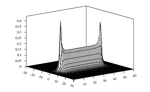
Figure 4: Electrical field strength $|\vec{E}|$ at $\lambda=2$

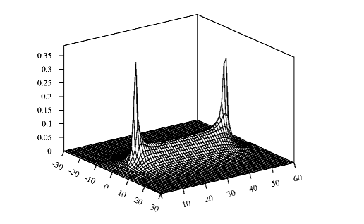
Figure 5: Electrical field strength $|\vec{E}|$ at $\lambda=4$

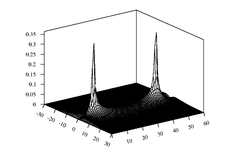
Figure 6: Electrical field strength $|\vec{E}|$ at $\lambda=8$

The actual density of monopole charges in a cut through the string is shown in fig. 7. Their concentration is largest just next to the string axis where the field is confined, and then drops sharply. This justifies the interpretation that the monopole charges create a “wall” that confines the electric field.

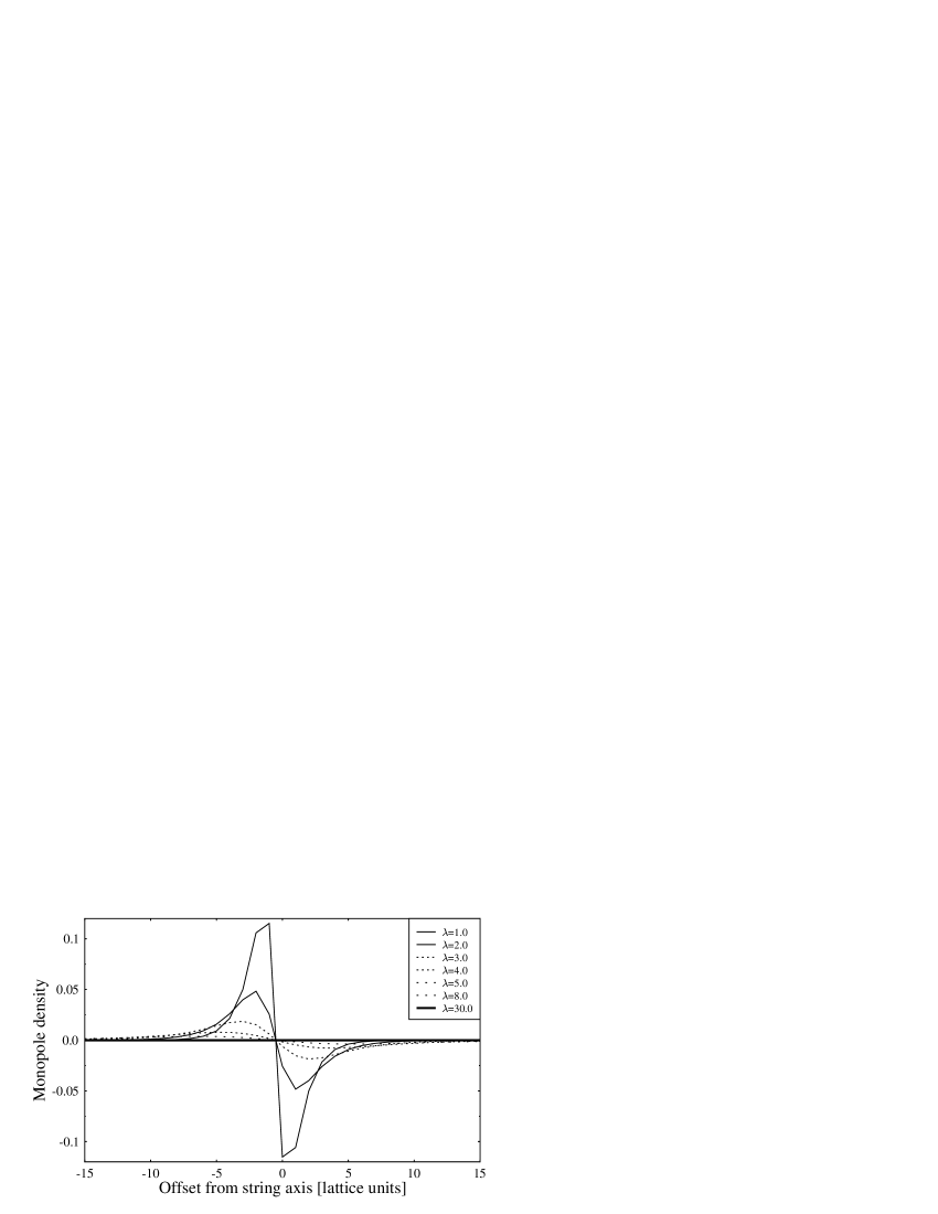
Figure 7: Monopole density in a cut across the string axis for different $\lambda$

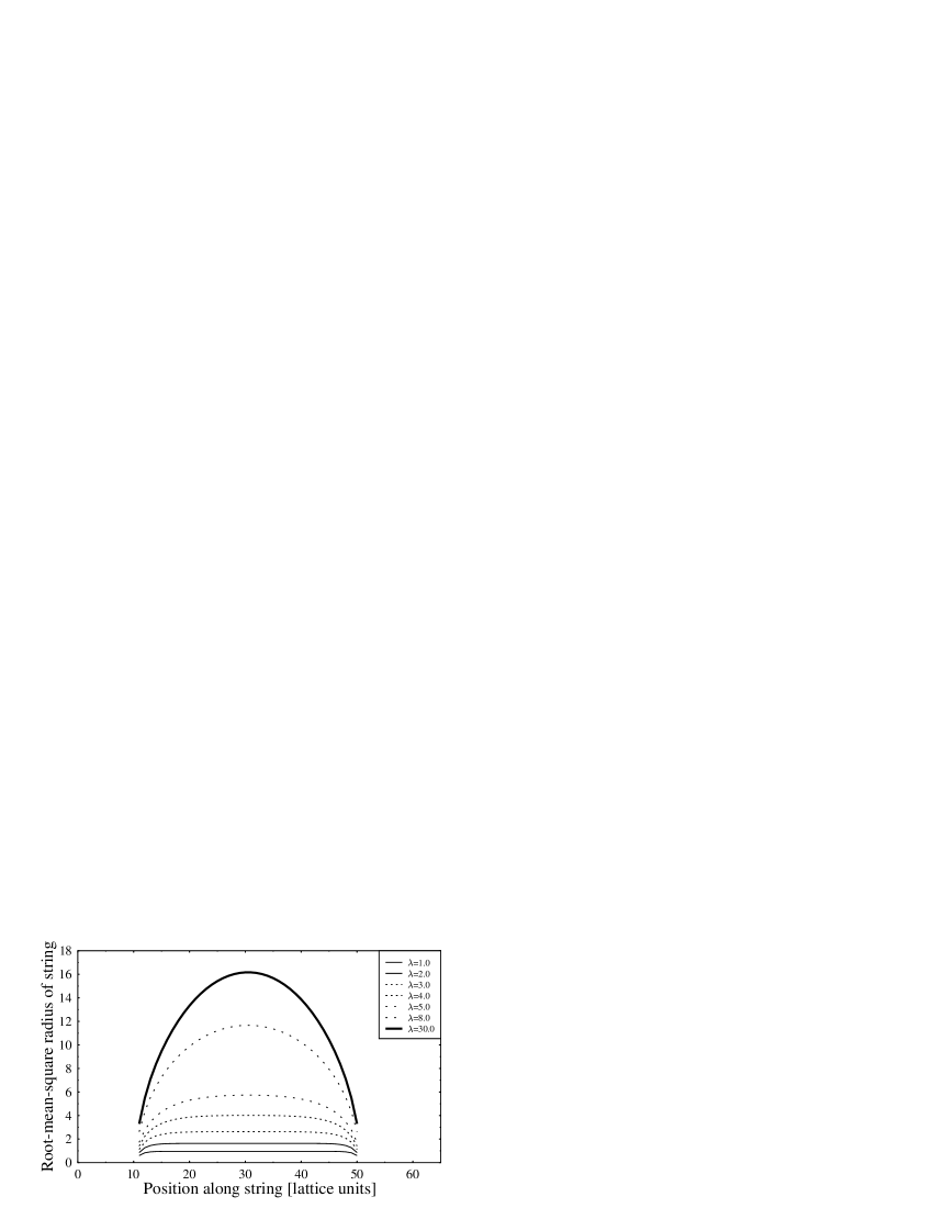
Figure 8: Root-mean-square radius of the string along the string axis for different values of $\lambda$

Figure 9: Root-mean-square radius of the string along the string axis for different distances of the charges

In fig. 8, we have calculated the root-mean-square radius

$$\bar{r}(x)=\sqrt{\frac{\sum_{y}y^{2}\,E_{x}^{2}(x,y)}{\sum_{y}E_{x}^{2}(x,y)}}$$ (53)

(where $y$ is the distance from the string axis) orthogonal to the string axis of the flux tube as a function of $\lambda$ and of the position along the string axis. For large $\lambda$, it is constant along most of the string axis, indicating the formation of a flux tube. For small $\lambda$, it smoothly reaches a maximum halfway between the charges as a result of the $1/r$-law.

Fig. 9 shows the root-mean-square radius for different lengths of the string. We do not see the $\ln r$ dependence [26] predicted from studying quantum fluctuations of the string. The width of the string stays constant, as would be expected from strong-coupling expansions. This is an indication that quantum effects will modify eq. (43).

The numerical solution of eq. (43) exhibits flux tube formation as is expected for confinement. As $\lambda$ is increased and the weak-coupling limit is approached, the flux tube disappears. On the other hand, it is expected from studies of the effective monopole action that $2+1$-dimensional $U(1)$ lattice gauge theory should not exhibit a phase transition to deconfinement [27]. Both results can be reconciled when considering that confinement of the electric field does not at first hand prove confinement of charges or provide for the calculation of the string tension. For the latter, it has to be shown that the ground-state energy of the Hamiltonian grows proportional to the distance of the charges. However, when truncating to single-plaquette states, any information about the correlation energy is lost, and the ground-state energy cannot be calculated reliably (cf. eq. (27)). For such a calculation, blocked ground states as used in real-space renormalization must be utilized, and the renormalization group, which is supposed to be the prime cause for confinement of charges, is brought back in. Quantum effects manifested by a roughening transition might then modify eq. (43) to reinforce confinement of the electric field.

4 Conclusions

We have shown that a semiclassical confining field equation can be directly derived from the Hamiltonian formulation of lattice gauge theory. Its linearized form is a London relation between the electric field and the monopole current. Numerical calculations show the formation of a flux tube for the electric field between two charges. The wall of the flux tube is formed by effective monopole currents that result from the nonlinearities of the field equation.

These results have been obtained using a rather crude discorrelated vacuum state. One of the major questions that accompanies this approach is how this equation is modified by correlations, i.e. quantum effects, and how this is related to a possible roughening transition [26]. The validity of the London relation for strong coupling has been demonstrated in Monte Carlo calculations. For weak coupling, renormalization group analysis predicts continued confinement of charges while the semiclassical field equations converge to the limit of classical electrodynamics. Here the inclusion of correlations (and consequently the renormalization group behavior) is needed to calculate the string tension and show confinement of charges. The most promising way to do this is to extend the truncation scheme to correlated blocks and perform a Hamiltonian real-space renormalization group analysis.

A direct check of the validity of eq. (43) is possible by comparing the results to Monte Carlo simulations. In particular, we are investigating the guided random-walk ground-state ensemble projector method [24] that is based on the Hamiltonian approach.

Further extension of the model is to $3+1$ dimensions and to the $SU(2)$ gauge group. In the extension to $3+1$ dimensions, one encounters constraints in the plaquette representation (Bianchi identities). While this will probably affect correlations, it remains to be seen whether the effective field equations changes qualitatively, and how this can be related to the maximally Abelian gauge which has been used in some of the Monte Carlo calculations.

Finally the extension to finite temperature can be considered to study the deconfinement transition.

This work was supported by Deutsche Forschungsgemeinschaft (DFG). C. B. wishes to thank the German National Scholarship Foundation for its support.

References

- [1] G. S. Bali, K. Schilling, Phys. Rev. D47, 661 (1993), hep-lat/9208028.
- [2] UKQCD Collaboration, Nucl. Phys. B 394, 509 (1992), hep-lat/9209007.
-
[3]
G.S. Bali, C. Schlichter, K. Schilling, Nucl. Phys. B (Proc. Suppl.) 34
(1994),
hep-lat/9311053.
G. Bali, C. Schlichter, K. Schilling, Phys. Rev. D51, 5165 (1995), hep-lat/9409005.
C. Schlichter, G. Bali, K. Schilling, Nucl. Phys. B (Proc. Suppl.) 273 (1995), hep-lat/9412018. -
[4]
V. Singh, D. A. Browne, R. W. Haymaker, Phys. Lett. B306, 115-119 (1993),
hep-lat/9301004.
R. W. Haymaker, V. Singh, Y.-C. Peng, hep-lat/9406021.
Y.-C. Peng, R. W. Haymaker, Phys. Rev. D52, 3030 (1995), hep-lat/9503015. - [5] G. ’tHooft, Physica Scripta 25, 133 (1982).
- [6] S. Mandelstam, Phys. Rep. 23C, 245 (1976).
- [7] M. Baker, J. S. Ball, F. Zachariasen, Phys. Rev. D 34, 3824 (1986); Phys. Rep. 209, 73 (1991).
- [8] T. Banks, R. Myerson, J. Kogut, Nucl. Phys. B 129, 493 (1977).
-
[9]
R. J. Wensley, J. D. Stack, Phys. Rev. Lett. 63, 1764 (1989).
J. D. Stack, R. J. Wensley, Nucl. Phys. B371, 597 (1992). - [10] G. ’tHooft, Nucl. Phys. B 190, 455 (1981).
- [11] T. A. DeGrand, D. Toussaint, Phys. Rev. D22, 2478 (1981).
- [12] V. Singh, R. W. Haymaker, D. A. Browne, Phys. Rev. D47, 1715 (1993), hep-lat/9206019.
- [13] A. Di Giacomo, M. Maggiore, S. Olejnik, Nucl. Phys. B347, 441 (1990).
- [14] P. Cea, L. Cosmai, Nucl. Phys. B (Proc. Suppl.) 42, 225 (1995).
- [15] L. DelDebbio, A. Di Giacomo, G. Paffuti, P. Pieri, Phys. Lett. B 349, 513 (1995).
- [16] K. G. Wilson, Phys. Rev. D14, 2455 (1974).
- [17] M. Zach, M. Faber, W. Kainz, P. Skala, Phys. Lett. B358, 325 (1995), hep-lat/9508017.
- [18] J. Kogut, L. Susskind, Phys. Rev. D11, 395 (1975).
- [19] C. J. Morningstar, M. Weinstein, Phys. Rev. Lett. 73, 1873 (1994), hep-lat/9405020.
- [20] C. H. Llewellyn Smith, N. J. Watson, Phys. Lett. B302, 463 (1993), hep-lat/9212025.
-
[21]
R. F. Bishop, Nucl. Phys. B (Proc. Suppl.) 34, 808 (1994).
R. F. Bishop, N. J. Davidson, Y. Xian, cond-mat/9411012. - [22] S. A. Chin, J. W. Negele, S. E. Koonin, Ann. Phys. 157, 140 (1984).
- [23] S. E. Koonin, E. A. Umland, M. R. Zirnbauer, Phys. Rev. D33, 1795 (1986).
- [24] C. Best, A. Schäfer, Nucl. Phys. B (Proc. Suppl.) 42, 216 (1995), hep-lat/9411076.
-
[25]
T. Suzuki, I. Yotsuyanagi, Phys. Rev. D42, 4257 (1990);
T. Suzuki, Nucl. Phys. B (Proc. Suppl.) 30, 176 (1993). -
[26]
M. Lüscher, G. Münster, P. Weisz, Nucl. Phys. B 180, 1 (1981).
G. Münster, P. Weisz, Nucl. Phys. B 180,13 (1981). - [27] A. M. Polyakov, Gauge Field and Strings, Harwood, Chur 1987.