DESY 96–003
HUB–EP–96/1
HLRZ 2/96
January 1996
The Status of Lattice Calculations of the Nucleon Structure Functions

Abstract

We review our progress on the lattice calculation of low moments of both the unpolarised and polarised nucleon structure functions.

1 INTRODUCTION

Much of our knowledge about QCD and the structure of nucleons has been derived from charged current Deep Inelastic Scattering (DIS) experiments in which a lepton (usually an electron or muon) radiates a virtual photon at large spacelike momentum $-q^{2}=Q^{2}$. This interacts with a nucleon (usually a proton) and measuring the total cross section yields information on $4$ structure functions for the nucleon – $F_{1}$, $F_{2}$ when polarisations are summed over and $g_{1}$, $g_{2}$ when the incident lepton beam and the proton have definite polarisations. The structure functions are functions of the Bjorken variable $x$ ($0\leq x\leq 1$) and $Q^{2}$. While the unpolarised case has been studied experimentally for many years (since the pioneering discoveries at SLAC), only recently have experiments been reported with polarised beams and targets ([1, 2]).

Theoretically, deviations from the simplest parton model (in which the hadron may be considered as a collection of non-interacting quarks) is taken as strong evidence for the evidence of QCD, where we have interacting quarks and gluons. A direct theoretical calculation of the structure functions seems not to be possible; however using the Wilson Operator Product Expansion (OPE) we may relate moments of the structure functions to matrix elements of certain operators in a twist or Taylor expansion in $1/Q^{2}$. For the unpolarised structure functions we find,

$$2\int_{0}^{1}\!dxx^{n-1}F_{1}(x,Q^{2})$$

$$= \sum_{f}E^{(f)}_{F_{1},n}v_{n}^{(f)}(\mu)+O(1/Q^{2}),$$

$$\int_{0}^{1}\!dxx^{n-2}F_{2}(x,Q^{2})$$ (1)

$$= \sum_{f}E^{(f)}_{F_{2},n}v_{n}^{(f)}(\mu)+O(1/Q^{2}),$$

where $n$ is even starting at $2$, $f=u,d,s,g$ and

$$\langle\vec{p},\vec{s}|{\cal O}^{\{\mu_{1}\cdots\mu_{n}\}}_{f}|\vec{p},\vec{s}\rangle=2v^{(f)}_{n}[p^{\mu_{1}}\cdots p^{\mu_{n}}-\mbox{\rm Tr}],$$ (2)

with

$${\cal O}^{\mu_{1}\cdots\mu_{n}}_{q} = \left(\frac{i}{2}\right)^{n-1}\bar{q}\gamma^{\mu_{1}}\stackrel{{\scriptstyle\leftrightarrow}}{{D}}^{\mu_{2}}\cdots\stackrel{{\scriptstyle\leftrightarrow}}{{D}}^{\mu_{n}}q,$$ (3)

$${\cal O}^{\mu_{1}\cdots\mu_{n}}_{g} = i^{n-2}\mbox{\rm{Tr}}F^{\mu_{1}\alpha}D^{\mu_{2}}\cdots D^{\mu_{n-1}}F^{\phantom{\alpha}\mu_{n}}_{\alpha}.$$

For the polarised structure functions,

$$2\int_{0}^{1}\!dxx^{n}g_{1}(x,Q^{2})$$

$$= {1\over 2}\sum_{f}E^{(f)}_{g_{1},n}a_{n}^{(f)}(\mu)+O(1/Q^{2}),$$

$$2\int_{0}^{1}\!dxx^{n}g_{2}(x,Q^{2})$$ (4)

$$= {1\over 2}{n\over{n+1}}\sum_{f}(E^{(f)}_{g_{2},n}d_{n}^{(f)}(\mu)-E^{(f)}_{g_{1},n}a_{n}^{(f)}(\mu))$$

$$+O(1/Q^{2}),$$

and

$$\langle\vec{p},\vec{s}|{\cal O}_{5f}^{\{\sigma\mu_{1}\cdots\mu_{n}\}}|\vec{p},\vec{s}\rangle$$

$$= {a^{(f)}_{n}\over{n+1}}[s^{\sigma}p^{\mu_{1}}\cdots p^{\mu_{n}}+\cdots],$$

$$\langle\vec{p},\vec{s}|{\cal O}_{5f}^{[\sigma\{\mu_{1}]\cdots\mu_{n}\}}|\vec{p},\vec{s}\rangle$$ (5)

$$= {d^{(f)}_{n}\over{n+1}}[(s^{\sigma}p^{\mu_{1}}-s^{\mu_{1}}p^{\sigma})p^{\mu_{2}}\cdots p^{\mu_{n}}+\cdots],$$

with

$${\cal O}_{5q}^{\sigma\mu_{1}\cdots\mu_{n}} = \left(\frac{i}{2}\right)^{n}\bar{q}\gamma^{\sigma}\gamma_{5}\stackrel{{\scriptstyle\leftrightarrow}}{{D}}^{\mu_{1}}\cdots\stackrel{{\scriptstyle\leftrightarrow}}{{D}}^{\mu_{n}}q,$$ (6)

$${\cal O}_{5g}^{\sigma\mu_{1}\cdots\mu_{n}} = i^{n-1}\mbox{\rm{Tr}}\tilde{F}^{\sigma\alpha}D^{\mu_{1}}\cdots D^{\mu_{n-1}}F^{\phantom{\alpha}\mu_{n}}_{\alpha}.$$

For $g_{1}$ we start with $n=0$, while for $g_{2}$ we begin with $n=2$ (${\cal O}_{5g},n=0$ is a special case).

While the Wilson coefficients, $E$, can be calculated perturbatively, the matrix elements cannot: a non-perturbative method must be employed. In principle lattice gauge theories provide such a method to compute these matrix elements from first principles. In this talk we shall describe our progress towards this goal, [3, 4], and try to discuss the problems that must be overcome. We will not dwell on lattice details and only give results in the form of Edinburgh (or APE) graphs which are plotted in terms of physical quantities.

The moments, eq. (1), have a parton model interpretation, being powers of the fraction of the nucleon momentum carried by the parton

$$v_{n}^{(q)}(\mu) = \langle x^{n-1}\rangle^{(q)}(\mu)$$

$$= \!\int_{0}^{1}\!dxx^{n-1}[q(x,\mu)+(-1)^{n}\bar{q}(x,\mu)],$$

where $q(x,\mu)=q_{\uparrow}(x,\mu)+q_{\downarrow}(x,\mu)$ (and similarly for $\bar{q}(x,\mu)$) with $q_{\updownarrow}(x,\mu)$ being the quark distributions at some scale $\mu$ and spin $\updownarrow$. For the gluon

$$v_{n}^{(g)}(\mu) = \langle x^{n-1}\rangle^{(g)}(\mu)$$ (8)

$$= \!\int_{0}^{1}\!dxx^{n-1}g(x,\mu).$$

Often we re-write the distributions in terms of valence, $v$ and sea, $S$ contributions ($q=u,d$),

$$q(x,\mu) \approx q_{v}(x,\mu)+S(x,\mu),$$

$$\bar{q}(x,\mu) \approx S(x,\mu),$$

$$s(x,\mu) \approx S(x,\mu),$$ (9)

assuming $SU_{F}(3)$ symmetry. While in $e(\mu)N$ DIS we can use only the charge conjugation positive moments (ie for even $n$), in $\nu N$ experiments we do not have this restriction and can use all moments. The lowest moment is particularly interesting, as due to conservation of the energy momentum tensor we have the sum rule $\sum_{q}\langle x\rangle^{(q)}+\langle x\rangle^{(g)}=1$.

For the polarised structure functions a similar interpretation holds for $g_{1}$,

$$a_{n}^{(q)}(\mu) = 2\langle x^{n}\rangle^{(q)}_{5}(\mu)$$

$$= 2\int_{0}^{1}\!dxx^{n}[\Delta q(x,\mu)+(-1)^{n}\Delta\bar{q}(x,\mu)],$$

where $\Delta q(x,\mu)=q_{\uparrow}(x,\mu)-q_{\downarrow}(x,\mu)$ (and similarly for $\Delta\bar{q}(x,\mu)$). The suitably modified eq. (9) is also taken to hold. Again the lowest moment is of particular interest because it can be related to the fraction of the spin carried by the quarks in the nucleon. Conventionally we define $\Delta q(\mu)$ by

$$\Delta q(\mu)=\int_{0}^{1}\!dx[\Delta q(x,\mu)+\Delta\bar{q}(x,\mu)],$$ (11)

and then

$$2\Delta q=a_{0}^{(q)}.$$ (12)

$g_{2}$ contains not only $a_{n}$ (the so-called Wandzura-Wilczek contribution to $g_{2}$) but also $d_{n}$ – a twist-$3$ contribution. It has been argued that the $n=0$ moment of $g_{2}$ should be $0$, but it is not possible to check this sum rule on a lattice. Finally we note that $g_{2}$ does not have a partonic interpretation.

2 THE APE PLOT

We shall now motivate the idea of an Edinburgh (or APE) plot. In a lattice calculation, we must first Euclideanise ($t\to-it$) and then discretise the QCD action and operators. This introduces a lattice spacing $a$ as an ultraviolet cutoff in addition to the (bare) coupling constant $\beta=6/g^{2}$ and for the Wilson formulation of lattice fermions, $1/\kappa$, which is related to the quark mass. (We shall only consider $m_{u}=m_{d}$ here.)

We first consider measuring the light hadron spectrum. Numerically we measure dimensionless numbers representing the different masses. In a region where scaling is taking place, [5], then

$${m_{h}^{phys}\over m_{h^{\prime}}^{phys}} = \left.{m_{h}\over m_{h^{\prime}}}\right|_{\mbox{\small{quark mass}}\equiv m_{\pi}/m_{N},m_{K}/m_{N},\ldots}$$ (13)

$$\stackrel{{\scriptstyle g^{2}\to 0}}{{\to}}$$ const.

Thus if we plot, for example $m_{N}/m_{\rho}$ as a function of $m_{\pi}/m_{\rho}$ (here we will take $m_{N}/m_{\rho}=f((m_{\pi}/m_{\rho})^{2}))$, we must be in a region where we see universal scaling, ie for different $g$ values the results lie on the same curve. The lattice spacing can be found from $a={m_{h}/m_{h}^{phys}}$.

Measuring the various masses yields the plot shown in Fig. 1

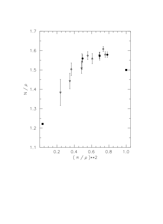
Figure 1: The APE plot $m_{N}/m_{\rho}$ against $(m_{\pi}/m_{\rho})^{2}$ for our results (filled circles, $\beta=6.0,16^{3}\times 32$ lattice), [4]. For comparison we also show the results of [6], (triangles, $\beta=6.0,18^{3}\times 32$ lattice), [7] (inverted triangles, $\beta=6.0,24^{3}\times 32$ lattice), and [8] (diamonds, $\beta=5.7,16^{3}\times 20$ lattice). The filled squares are the experimental result and heavy quark limit $(1,3/2)$.

The plot allows the whole range of quark mass to be shown, from the heavy quark mass limit to the physical point. In fact from the lattice many quark mass worlds can be computed. (Unfortunately everything except the real world: this is because the $u$ and $d$ quark masses are very close to the chiral limit, which numerically is difficult to realise.) Our lightest quark mass lies at about the mass of the strange quark (in the middle of the plot, $(m_{\pi}/m_{\rho})^{2}\approx 0.5$). Do we have universal scaling? Roughly the points seem to lie in a band – a good sign, although the smaller coupling values seem to lie slightly above the larger coupling value. Are there finite size effects? Looking at the lightest quark masses we see a slight dropping of the value when increasing the spatial lattice size. This might be interpreted as a sign of some finite volume effects. We note also the difficulty of linear extrapolations – using our results alone would give a rather different result to the physical result. Using lighter quark mass results as well gives a more satisfactory extrapolation, [4]. The curve from the heavy quark mass world to the physical world is certainly rather unpleasant – the curve first goes up before sinking down. We have also used the quenched approximation in which the fermion determinant is ignored (otherwise the computations are too costly). This introduces an uncontrolled approximation – for example it is thus not clear that the ratio in eq. (13) need be the physical value. Finally as we have a choice of which hadron mass to use to find $a$, if we are not in the neighbourhood of the physical point, we will get ambiguities in the value. From [4], we find $a\approx 2.0-2.5\mbox{GeV}^{-1}$ (using $m_{N}$, $m_{\rho}$).

3 LOW MOMENTS

We shall now present our results for the low moments of the structure functions. The computational method is to evaluate the nucleon two point functions with a bilinear quark or gluon operator insertion, leading to a numerical estimate of the matrix elements in eqs. (2,5). There are two basic types: The first is quark insertion in one of the nucleon quark lines (quark line connected). As this involves a valence quark, we shall take this as probing the valence distributions in eq. (9). In the second type the operator interacts via the exchange of gluons with the nucleon (for quark line disconnected and gluon operators). These are taken as probes of the sea and gluon distributions. (Of course as we work in the quenched approximation there may be some distortions in the various distributions.) Due to technical difficulties, such as the operator growing too large in comparison with the lattice spatial size and the mixing of the lattice operators with lower dimensional operators, it has only been possible to measure the lowest three quark moments for the unpolarised valence structure functions, to give an estimate for the lowest gluon moment and for the polarised valence structure functions to compute $a_{0}$, $a_{2}$ and $d_{2}$. (Some sea quark distributions also have been attempted in [8, 9].) After computation the lattice matrix elements must be renormalised. For this we use at present the one–loop perturbation results, [4]. (However improvements are being developed, [10].) Finally we shall quote all our results at the reference scale,

$$Q^{2}=\mu^{2}={1\over a^{2}}\approx 4-6\mbox{GeV}^{2}$$ (14)

(to avoid having to re-sum large logarithms in $Z$ or the Wilson coefficients).

Unpolarised

In Fig. 2 we show the APE plot for the $3$ lowest valence moments.

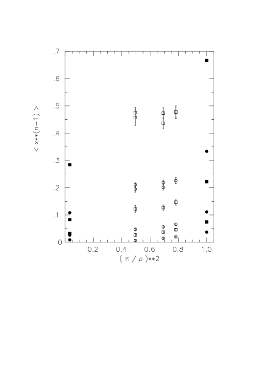
Figure 2: The APE plot for valence results: $\langle x^{n-1}\rangle^{(q)}$ with $n=2,3,4$, top to bottom, in turn first for the $u$ quarks (squares) and then for the $d$ quarks (circles). (For $\langle x\rangle$, we have evaluated the matrix elements in two distinct ways, [4], methods $a,b$.) The experimental numbers and heavy quark limit are the filled symbols.

Also shown are the physical values (taken from [11]) and the heavy quark mass limit $q_{\updownarrow,v}(x)\to c_{q_{\updownarrow}}\delta(x-1/3)$, $S(x)\to 0$. We see that the results roughly seem to lie on a smooth extrapolation from the heavy quark mass limit to the physical result. (Although the lightest quark mass seems to be levelling off, this should be checked on a larger lattice to see that there are no finite volume effects present.) It is to be hoped that smaller quark masses will continue to drift downwards. Certainly little sign of overshooting is seen (as happened in the APE mass plot). In Fig. 3 we show the ratios of the $u_{v}$ to $d_{v}$ moments.

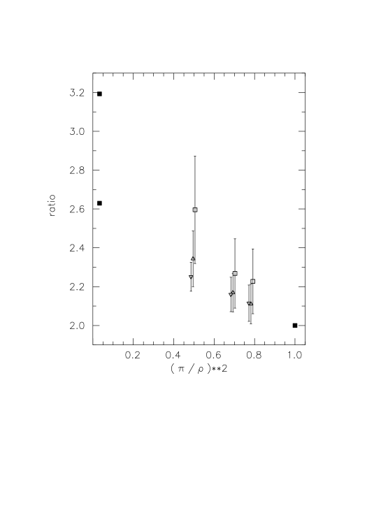
Figure 3: The APE plot for the ratio of the valence moments: $\langle x^{n-1}\rangle^{(u)}/\langle x^{n-1}\rangle^{(d)}$. Method $a$ ($n=2$) are triangles. Method $b$ (inverted triangles) and $n=3$ (squares) are slightly displaced for clarity.

There seem indications of a very smooth (linear?) behaviour with the quark mass. In Fig. 4 we show the lowest gluon moment.

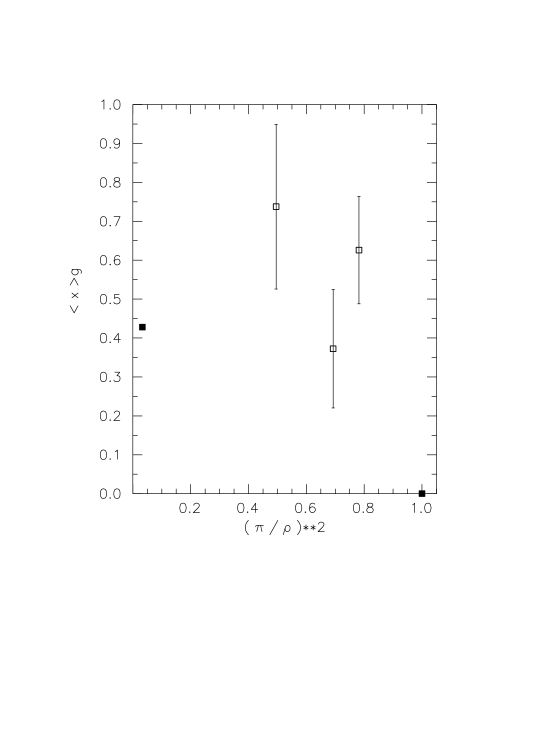
Figure 4: The APE plot for $\langle x\rangle^{(g)}$.

The experimental result comes from [12]. (In the heavy quark mass limit we would expect all the nucleon momentum to reside in the quarks and none in the gluons.) At present the signal is not so good. This is numerically a difficult calculation however and requires a large statistic. No statement at present can be made on the momentum sum rule.

Polarised

We now turn to a consideration of the polarised structure function moments. We first consider the non-singlet results for $a_{0}$. The octet and triplet currents are given by

$$3F_{A}-D_{A}=\Delta u+\Delta d-2\Delta s\approx\Delta u_{v}+\Delta d_{v}$$

$$F_{A}+D_{A}=g_{A}=\Delta u-\Delta d\approx\Delta u_{v}-\Delta d_{v}$$ (15)

and thus we need only look at connected diagrams. Space prevents us from showing results for $g_{A}$, $3F_{A}-D_{A}$ or $F_{A}/D_{A}$, we refer the interested reader to the nice review [13]. (Comparing the results there with the experimental and the heavy quark mass limit we again see for $g_{A}$ an overshoot effect: we seem to have to climb up to reach the experimental value.) For the singlet results we have $\Delta u+\Delta d+\Delta s\equiv\Delta\Sigma$ and so we expect the disconnected terms to be more important. This is a very difficult problem, [8, 9]. Recent numerical estimates however show an encouraging trend to the experimental result, [13].

Of the higher $a$ moments we have been able to look at $a_{2}$. Changing to $p=\mbox{proton}$, $n=\mbox{neutron}$ (rather than $u$, $d$), we plot $a_{2}$ in Fig. 5.

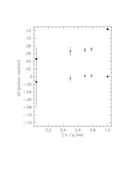
Figure 5: The APE plot for $a_{2}^{p,n}$. The squares are the proton results, while the circles are the neutron results.

(The numbers for $a_{2}$ and $d_{2}$ are conveniently collated in [14].) Again we see a rather smooth behaviour between the heavy quark mass limit and the experimental result. Indeed, perhaps due to the present rather large errors there, we could claim that we have reasonable agreement with experiment.

Finally we turn to an estimation of $d_{2}$ – the first non-leading twist operator in the OPE expansion. In Fig. 6 we plot our

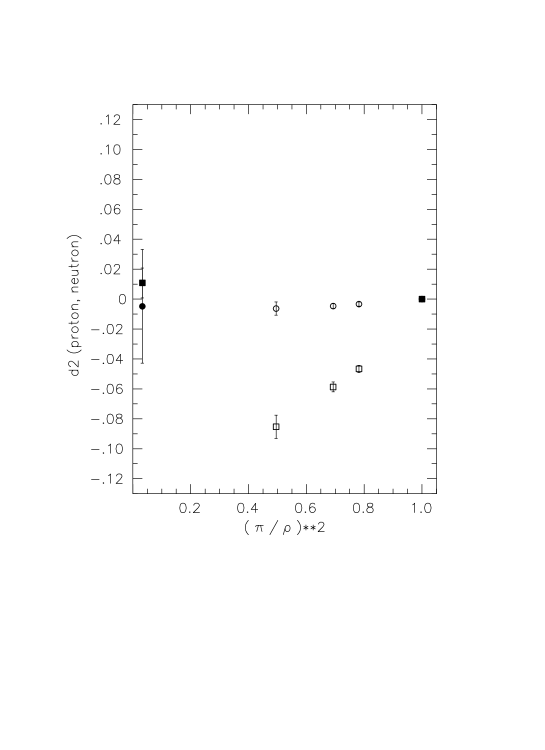
Figure 6: The APE plot for $d_{2}^{p,n}$. The same notation as for Fig. 5.

results. While one might say that for $n$ we are compatible with the experimental result, for $p$ we have crass disagreement. At present we have no explanation for this result. (Indeed as we tend towards the chiral limit, the discrepancy grows.) In Fig. 7

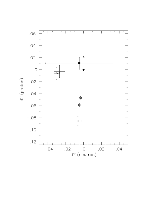
Figure 7: $d_{2}^{(p)}$ versus $d_{2}^{(n)}$. The lattice results are shown as squares, sum rule as (inverted ) triangles, and the bag estimate as a diamond. The experimental value is a filled square and the heavy quark mass limit is a filled circle.

we compare our results with other theoretical estimates. At present the lattice result comes out a poor last. (But one should note that the most compatible result to the experiment appears to be the heavy quark mass limit.)

Conclusions

Although progress has been made, it is clear that much more remains to be done. In particular for reliable extrapolations to the chiral limit, smaller quark mass simulations are necessary.

References

- [1] J. Ashman et al., Nucl. Phys. B238 (1990) 1.
- [2] K. Abe et al., Phys. Rev. Lett 75 (1995) 346, ibid 75 (1995) 25; hep-ex/9511013.
- [3] M. Göckeler et al., Nucl. Phys. B(Proc. Suppl.) 42 (1995) 337, (hep-lat/9412055); Yamagata Workshop (hep-lat/9509079); Lat95 (hep-lat/9510017); Brussels HEP Conference (hep-lat/9511013); Zeuthen Spin Workshop (hep-lat/9511025).
- [4] M. Göckeler, R. Horsley, E.-M. Ilgenfritz, H. Perlt, P. Rakow, G. Schierholz and A. Schiller, hep-lat/9508004 (accepted for PRD).
- [5] R. D. Kenway, QCD years later, Aachen, 1992.
- [6] S. Cabasino et al. Phys. Lett. B214 (1988) 115.
- [7] S. Cabasino et al. Phys. Lett. B258 (1991) 195.
- [8] M. Fukugita et al., Phys. Rev. Lett. 75 (1995) 2092, (hep-lat/9501010).
- [9] S. J. Dong et al., Phys. Rev. Lett. 75 (1995) 2096, (hep-lat/9502334).
- [10] G. Martinelli et al., Nucl. Phys. B445(1995) 81, (hep-lat/9411010).
- [11] A. Martin et al., Phys. Rev. D47 (1993) 867.
- [12] A. D. Martin et al., Phys. Lett. B354 (1995) 155, (hep-ph/9502336).
- [13] M. Okawa, Lat95 (hep-lat/9510047).
- [14] L. Mankiewicz et al., Zeuthen Spin Workshop (hep-ph/9510418).