Chiral symmetry at finite $T$, the phase of the Polyakov loop and the spectrum of the Dirac operator.

Abstract

A recent Monte Carlo study of quenched QCD showed that the chiral condensate is non-vanishing above $T_{c}$ in the phase where the average of the Polyakov loop $P$ is complex. We show how this is related to the dependence of the spectrum of the Dirac operator on the boundary conditions in Euclidean time. We use a random matrix model to calculate the density of small eigenvalues and the chiral condensate as a function of $\arg P$. The chiral symmetry is restored in the $\arg P=2\pi/3$ phase at a higher $T$ than in the $\arg P=0$ phase. In the phase $\arg P=\pi$ of the $SU(2)$ gauge theory the chiral condensate stays nonzero for all $T$.

I Introduction

The relation between chiral symmetry breaking and confinement in gauge theories has been a subject of continuous interest. The picture of chiral symmetry breaking suggested by Banks and Casher [1] relates the chiral condensate to the average density of small eigenvalues of the Dirac operator in the fluctuating background of the gauge field. The appearance of small eigenvalues in turn can be related to the fact that the QCD vacuum is populated by instanton configurations [2].

The pure QCD without quarks undergoes a phase transition at some temperature $T_{c}$. It is interesting to see whether this transition affects the behavior of small eigenvalues of the Dirac operator in such a way that the chiral symmetry is restored. This motivates a Monte Carlo study of QCD with quenched quarks. In this paper we analyze the recent result [3] of such a study. Unlike previous similar works [4] the authors looked at the value of the chiral condensate in each of the $Z_{3}$ symmetric directions in the complex plane in which the Polyakov loop acquires a nonzero expectation value above $T_{c}$. It was found that:

• The chiral condensate $\langle\bar{\psi}\psi\rangle$ vanishes above $T_{c}$ in the phase with $\arg P=0$.

• In the phase with the $\arg P=2\pi/3$ the $\langle\bar{\psi}\psi\rangle$ is nonzero for some range of $T>T_{c}$ !

The last point (b) contradicts a naive expectation that the vanishing of the $\langle\bar{\psi}\psi\rangle$ has something to do with the rearrangement of the QCD equilibrium state at $T_{c}$, e.g., a suppression of the instanton configurations in the deconfined phase. In this paper we show that this result can indeed be explained very naturally if one takes into account only the effect of the boundary conditions on the quark fields in the Euclidean time. Nevertheless the fact (a) that the vanishing of $\langle\bar{\psi}\psi\rangle$ coincides with $T_{c}$ tells us that the rearrangement of the QCD equilibrium state at $T_{c}$ also plays a role.

II Polyakov loop and the spectrum of the Dirac operator

The partition function of the QCD without quarks can be written as a Euclidean path integral:

$$Z=\int{\cal D}A_{\mu}\exp\{-S[A]\};\qquad S=\int_{0}^{1/T}\int d^{3}\mbox{\boldmath$x$}F_{\mu\nu}F_{\mu\nu}.$$ (1)

An order parameter distinguishing the confined and the deconfined phases is the expectation value of the Polyakov loop:

$$P(\mbox{\boldmath$x$})={1\over 3}\mbox{ Tr }\mbox{ P}\exp\left\{ig\int_{0}^{1/T}\,dt\,A_{0}(t,\mbox{\boldmath$x$})\right\},$$ (2)

The value of $P$ is invariant under a gauge transformation periodic in the Euclidean time: $U(1/T)=U(0)$. However, the action $S$ is also invariant under aperiodic gauge transformations:

$$U(1/T)=zU(0),$$ (3)

with $z=I\exp\{i2\pi/3\}$, which do not upset the boundary conditions on $A_{\mu}$ because $z$ commutes with all matrices in the gauge group. The value of the Polyakov loop acquires a phase $\exp\{i2\pi/3\}$ after such a transformation. This corresponds to a $Z_{3}$ symmetry transformation in an effective theory of the Polyakov loops.

At small temperatures the expectation value of the Polyakov loop is zero and the $Z_{3}$ symmetry is exact. Above $T_{c}$ the Polyakov loop acquires a non-vanishing expectation value which can be related to the liberation of color [5].

           

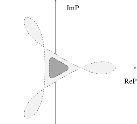
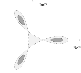
(a)                                                      (b)

FIG. 1.: A schematic contour plot of the distribution of the averaged value of the Polyakov loop: (a) — below $T_{c}$, (b) — above $T_{c}$. Only 2 isolines are drawn: one at the level of the saddle point between the peaks and another in between the heights of the peaks.

To analyze the results of the Monte Carlo simulation it is helpful to consider a probability distribution of the Polyakov loop in a large but finite volume. It can be calculated as a histogram [6]: For each configuration one finds the averaged (over $x$) $P$. The configuration then contributes a unit to the height of the histogram at this $P$. The qualitative behavior near $T_{c}$ of this distribution is shown in Fig. 1. There are 4 peaks. At low $T$ the peak at $P=0$ is taller. Most of the configurations have very small $P$ near the origin. At $T=T_{c}$ the 3 degenerate peaks at nonzero $P$ are (roughly) of the same height as the peak at the origin. At higher $T$ the $Z_{3}$ peaks are taller.

The chiral condensate is measured by averaging the inverse of the Dirac operator over the gauge configurations. At high $T$ one has a choice of averaging over ensembles of configurations clustered near each of the $Z_{3}$ peaks. We refer to these ensembles as $Z_{3}$ phases. It was found in [3] that the result is different in the phases $\arg P=0$ and $\arg P=2\pi/3$.

Due to the $Z_{3}$ symmetry an ensemble of gauge configurations in the phase $\arg P=2\pi/3$ can be mapped onto the ensemble at $\arg P=0$ by an aperiodic gauge transformation (3). The $Z_{3}$ phases of pure QCD are equivalent. However, the spectrum of the Dirac operator is not invariant under such a transformation. We conclude that different behavior of the chiral condensate in the two phases is entirely due to the effect of the aperiodic gauge transformation on the spectrum of the Dirac operator.

The action of the gauge transformation (3) on the fermion fields changes the boundary conditions in the Euclidean time direction from antiperiodic:

$$\psi(1/T,\mbox{\boldmath$x$})=-\psi(0,\mbox{\boldmath$x$})$$ (4)

to twisted:

$$\psi(1/T,\mbox{\boldmath$x$})=-z\psi(0,\mbox{\boldmath$x$}).$$ (5)

The eigenvalue problem for the Dirac operator is defined by the differential equation:

$$(D/+m)\psi=\lambda\psi,$$ (6)

with functions $\psi(x)$ satisfying given b.c. The b.c. in this problem are different in the phases with $\arg P=0$ and $\arg P=2\pi/3$.

Moreover, qualitatively one can see that the effect of a nontrivial $Z_{3}$ phase on the b.c. tends to lower the eigenvalues, because of less twisting required of $\psi$. It is transparent if you consider as an example the free Dirac operator, i.e. $A_{\mu}=0$. In this case, the spectrum in the phase $\arg P=0$ is given by: $\lambda^{2}=\mbox{\boldmath$k$}^{2}+((2n+1)\pi T)^{2}$. While in the $\arg P=2\pi/3$ phase it becomes: $\lambda^{2}=\mbox{\boldmath$k$}^{2}+((2n+1/3)\pi T)^{2}$. The smallest eigenvalue moves from $\lambda=\pi T$ to $\lambda=\pi T/3$.

III Random matrix model

To find the dependence of the spectrum on $\arg P$ for arbitrary $A_{\mu}$ is a very difficult problem. Fortunately, the only information we need about the spectrum is the density of small eigenvalues $\rho(\lambda\to 0)$ which is related to the chiral condensate by [1]:

$$\langle\bar{\psi}\psi\rangle=\pi\rho(0).$$ (7)

To go further we need to make some approximations. As our first approximation we neglect the Euclidean time dependence of the gauge configurations responsible for small eigenvalues. This is not altogether unreasonable approximation at least at $T$ of the order of $T_{c}$ and higher for the following two reasons. First, it is the infrared behavior of the gauge fields that is responsible for the small eigenvalues. It is known, that the IR behavior of QCD at high $T$ is given by a 3-dimensional theory [7]. Second, the correlation length at the first order phase transition in pure QCD may be large compared to $1/T$ — the extent in the time direction. For the $SU(3)$ theory this is suggested by the fact that in the Potts model, to which this transition is related by universality arguments, the transition is very weakly first order. For the $SU(2)$ theory the correlation length is infinite at $T_{c}$ and the theory is effectively 3-dimensional at $T_{c}$.

In this approximation we can separate $t$ and $x$ dependence in the eigenfunctions: $\psi(t,\mbox{\boldmath$x$})=\sum_{n}e^{i\omega_{n}t}\psi_{n}(\mbox{\boldmath$x$})$. Thus (6) reduces to the eigenvalue problem for a three-dimensional operator:

$$[i\gamma_{0}\omega_{n}+i\gamma_{0}A_{0}+\mbox{\boldmath$\gamma D$}+m]\psi_{n}(\mbox{\boldmath$x$})=\lambda\psi_{n}(\mbox{\boldmath$x$})$$ (8)

for each $\omega_{n}$, where the gauge fields $A_{0}$, $A$ depend only on $x$. The values of $\omega_{n}$ are determined by the b.c. in the Euclidean time:

$$\omega_{n}=((2n+1)\pi-\arg P)T.$$ (9)

To find the density of small eigenvalues (or, chiral condensate) for the operator (8) we use another approximation known as the (Gaussian) random matrix model [8]. We choose a basis $\psi_{a}$ of $N$ functions (the same for all gauge field configurations and all $\omega_{n}$) and write the three-dimensional Dirac operator in this basis:

$$\left(\begin{array}[]{cc}m&iX+i\omega_{n}\\ iX^{\dagger}+i\omega_{n}&m\end{array}\right),$$ (10)

where the $X$ is a complex $N\times N$ matrix. Then one can replace the averaging over the gauge fields by averaging over the elements of the matrix $X$. The main approximation of the model, which proves to be very good (and, probably, exact in some sense) in 4d [8], is that the probability distribution is Gaussian. In other words, we calculate:

$$Z=\int{\cal D}X\exp\left\{-{NC^{2}}\,{\rm Tr}\,XX^{\dagger}\right\}\prod_{n}{\det}^{N_{f}}\left(\begin{array}[]{cc}m&iX+i\omega_{n}\\ iX^{\dagger}+i\omega_{n}&m\end{array}\right).$$ (11)

This is actually an approximation to the full partition function of QCD with $N_{f}$ flavors of dynamical fermions. We will be interested, however, in the limit $N_{f}\to 0$ — quenched fermions. In fact, one can check that $N_{f}$ cancels out in our final results anyway. Therefore, to simplify the formulae we shall put $N_{f}=1$. It is also convenient to view each Matsubara mode as a flavor with a Matsubara mass $\omega_{n}$. From $Z$ we can obtain the chiral condensate in the thermodynamic limit:

$$\langle\bar{\psi}\psi\rangle=\lim_{m\to 0}\lim_{V_{3}\to\infty}{T\over N_{f}V_{3}}{\partial\over\partial m}\ln Z.$$ (12)

where $V_{3}$ is the volume of the 3-space.

The calculation [8, 9] of (11) is similar in spirit to the mean field calculation in the large $N$ sigma models (Hubbard-Stratonovich transformation). We introduce a new random matrix $Y$, the integral over which can be calculated in the saddle point approximation at large $N$. The first step is to rewrite the determinant as a Grassmann integral:

$$Z=\int{\cal D}X{\cal D}\bar{\Psi}{\cal D}\Psi\exp\left\{-NC^{2}\mbox{ Tr }XX^{\dagger}\right\}\exp\left\{\sum_{n}\bar{\Psi}_{n}\left(\begin{array}[]{cc}m&iX+i\omega_{n}\\ iX^{\dagger}+i\omega_{n}&m\end{array}\right)\Psi_{n}\right\}.$$ (13)

The spinors $\Psi^{a}_{n}$ carry an implicit index $a$ ($a=1,\ldots,N$). Integration over $X_{ab}$ can be carried out which creates the four-fermion term:

$$-{1\over NC^{2}}\bar{\Psi}^{a}_{Ln}\Psi^{b}_{Rn}\bar{\Psi}^{b}_{Rm}\Psi^{a}_{Lm}.$$ (14)

This term can be rewritten using another auxiliary random matrix $Y_{mn}$:

$$Z=\int{\cal D}Y{\cal D}\bar{\Psi}{\cal D}\Psi\exp\left\{-NC^{2}\mbox{ Tr }YY^{\dagger}\right\}\exp\left\{\sum_{a=1}^{N}\bar{\Psi}^{a}\left(\begin{array}[]{cc}Y+m&iM\\ iM&Y^{\dagger}+m\end{array}\right)\Psi^{a}\right\},$$ (15)

where $M$ is a diagonal matrix $\omega_{n}\delta_{nk}$.

The integral over Grassmann variables can be then performed:

$$Z=\int{\cal D}Y\exp\left\{-NC^{2}\mbox{ Tr }YY^{\dagger}\right\}{\det}^{N}\left(\begin{array}[]{cc}Y+m&iM\\ iM&Y^{\dagger}+m\end{array}\right).$$ (16)

At large $N$ the saddle point equation for the matrix $Y$ is:

$$-C^{2}Y+(Y+m)\left[(Y^{\dagger}+m)(Y+m)+M(Y+m)^{-1}M(Y+m)\right]^{-1}=0.$$ (17)

This has a solution in the form of a diagonal matrix with eigenvalues $y_{n}$ that satisfy (we put m=0 here):

$$C^{2}y_{n}={y_{n}\over\omega_{n}^{2}+y_{n}^{2}}.$$ (18)

This equation is analogous to the well known gap equation in the large $N$ sigma models. A nontrivial solution $y_{n}=(1/C)\sqrt{1-\omega_{n}^{2}C^{2}}$ exists only for those $n$ for which: $1-\omega_{n}^{2}C^{2}>0$.

Using (12) and (16) we find that the chiral condensate is given by:

$$\langle\bar{\psi}\psi\rangle=\lim_{m\to 0}\lim_{V_{3}\to\infty}{T\over V_{3}}\left\langle N\mbox{ Tr }\left(\begin{array}[]{cc}Y+m&iM\\ iM&Y^{\dagger}+m\end{array}\right)^{-1}\right\rangle.$$ (19)

In the saddle point approximation at large $N$ using (18) we find:

$$\langle\bar{\psi}\psi\rangle=n_{3}C\sum_{n}\sqrt{1-\omega_{n}^{2}C^{2}}\cdot\theta(1-\omega_{n}^{2}C^{2}),$$ (20)

where $n_{3}=2N/V_{3}$ and $\omega_{n}=((2n+1)\pi-\arg P)T$.

We see that the chiral condensate vanishes (continuously: $\beta=1/2$ in this approximation) when $\min_{n}|\omega_{n}|>1/C$, in other words, when the temperature exceeds:

$$T_{\chi}(\arg P)={1\over C|\pi-\arg P|},$$ (21)

where $\arg P$ is mod $2\pi$. This result is in accordance with our expectation that nonzero $\arg P$ favors chiral symmetry breaking.

Our model at $\arg P=0$ is similar to a model suggested in [9] where only the lowest Matsubara frequency was taken into account. This makes sense since we are interested in the behavior of small eigenvalues of the Dirac operator. Indeed, only the band $\omega_{0}$ of the eigenvalues contributes in (20) when $T$ is close to $T_{\chi}$ and $0<\arg P<2\pi$. In our case keeping all Matsubara frequencies ensures periodicity in $\arg P\bmod 2\pi$.

IV Discussion and conclusions

We analyzed a recent Monte Carlo observation that the chiral condensate $\langle\bar{\psi}\psi\rangle$ does not vanish in some interval above $T_{c}$ in quenched QCD in the phase with $\arg P=2\pi/3$. This fact suggests that the rearrangement of the QCD equilibrium state at $T_{c}$ (deconfinement) is not the only source of the restoration of the chiral symmetry in quenched QCD.

We calculated (approximately) the chiral condensate at finite $T$ taking into account the dependence of the spectrum of the Dirac operator on the b.c. for the quark fields in the Euclidean time. We found that the $\langle\bar{\psi}\psi\rangle$ vanishes continuously at a temperature $T_{\chi}(\arg P)$ which depends on the phase of the Polyakov loop (21).

This suggests the following interpretation of the result [3]. As we approach the deconfinement transition from $T>T_{c}$ side the chiral symmetry breaking in the $\arg P=2\pi/3$ phase occurs earlier, at a temperature $T_{\chi}(2\pi/3)>T_{c}$. The chiral condensate is zero in the $\arg P=0$ phase because $T_{\chi}(0)<T_{\chi}(2\pi/3)$. It turns out that $T_{c}>T_{\chi}(0)$. Indeed, the result [3] suggests that $T_{c}$ is only about 7% lower than $T_{\chi}(2\pi/3)$, while in our approximation $T_{\chi}(0)$ is about $1/3$ of $T_{\chi}(2\pi/3)$. At $T_{c}$ the $Z_{3}$ phases become metastable and at lower temperatures the single $P=0$ phase dominates (see Fig. 1).

Being cavalier enough, one can conjecture that the effect of this transition on $\langle\bar{\psi}\psi\rangle$ can be taken into account very roughly by averaging over 3 values of $\arg P$. This would lead to a relation between the condensate just below $T_{c}$ and the condensate in the $\arg P=2\pi/3$ phase just above $T_{c}$:

$$\langle\bar{\psi}\psi\rangle(T_{c}-)\approx{2\over 3}\langle\bar{\psi}\psi\rangle(T_{c}+,\arg P=2\pi/3),$$ (22)

which does not seem to be in a gross contradiction with [3]. In other words, 3 phases of the Polyakov loop “mix together” below $T_{c}$.

In a picture of the chiral phase transition in the quenched QCD suggested here the restoration of the chiral symmetry at finite $T$ is mainly due to the effect of the b.c. in the Euclidean time suppressing small eigenvalues of the Dirac operator. The rearrangement of the QCD equilibrium state plays a secondary role. This goes in line with the fact that, as far as we know, the instanton density behaves rather smoothly across the phase transition [2, 10, 11]. The effect of the b.c. in the $\arg P=0$ phase is stronger than in the $\arg P=2\pi/3$ phase and in the low temperature $P=0$ phase. To put this into another perspective one can note that antiperiodic boundary conditions for the quark fields are related to the Pauli exclusion principle. The fact that Pauli blocking leads to chiral symmetry restoration is rather well known in various models of particle and nuclear physics.

Another interesting consequence of (21) is that in the $SU(2)$ gauge theory: $T_{\chi}(\pi)=\infty$. This means that the $\langle\bar{\psi}\psi\rangle$ stays nonzero for all $T$ in the $\arg P=\pi$ phase!

This result can be argued for also beyond the approximation of the random matrix model. Recall that the theory at very high $T\gg T_{c}$ becomes effectively 3-dimensional. Moreover, fermions which would “decouple” in the $\arg P=0$ phase do not in the $\arg P=\pi$ phase because the b.c. are periodic. Thus the value of $\langle\bar{\psi}\psi\rangle$ is determined by the 3-dimensional $SU(2)$ gauge theory at zero temperature. The value of the $\langle\bar{\psi}\psi\rangle$ is nonzero in such a theory [12]. Moreover, it can be estimated to be of the order of $g_{3}^{4}$ purely on dimensional grounds. This means that the chiral condensate in the $SU(2)$ theory in the $\arg P=\pi$ phase at $T\gg T_{c}$ is of the order:

$$\langle\bar{\psi}\psi\rangle\sim g^{4}T^{3}.$$ (23)

Recently there have been two attempts [14, 15] to describe the data [3] using a Nambu-Jona-Lasinio model. With some tuning of parameters it is possible to achieve a reasonable fit to the data in the model [15]. The present paper emphasizes the role of the behavior of small eigenvalues as a function of $\arg P$ and in this respect differs from a somewhat phenomenological approach of [14, 15]. This allows us to obtain new results, for example, (21) or (23).

It would be interesting to test these results in a Monte Carlo simulation. For example, one can consider b.c. conditions on fermions with an arbitrary twist. This would add to our knowledge of the mechanism of the chiral symmetry restoration in QCD.

Acknowledgments:  The author would like to thank A. Kocic, J. Kogut, C. Korthals-Altes and R. Pisarski (who brought the result [3] to the author’s attention) for useful discussions and comments and the theory group of the Brookhaven National Laboratory for hospitality. The work was supported by the NSF grant PHY 92–00148.

A The density of eigenvalues

The eigenvalue density $\rho(\lambda)$ for the Dirac operator can be found in a closed form in our approximation. Let us consider only the lowest band of eigenvalues with $\omega=\min_{n}|\omega_{n}|$. Contributions of the other bands are additive. To find $\rho(\lambda)$ we note that one can calculate $\langle\bar{\psi}\psi\rangle(m)$ for arbitrary $m$. On the other hand, $\rho(\lambda)$ is the discontinuity of $\langle\bar{\psi}\psi\rangle(m)$ along the imaginary axis, in other words:

$$\mbox{ Re }\langle\bar{\psi}\psi\rangle(i\lambda+\epsilon)=\pi\rho(\lambda).$$ (A1)

The $\langle\bar{\psi}\psi\rangle(m)$ is given by (19) if we do not take $m\to 0$. The necessary eigenvalue $y$ can be found from (17) by solving a cubic equation. Finally, we obtain:

$${\pi\rho(\lambda)\over C}={\sqrt{3}\over 2}\left[({\sqrt{\Delta}}+q)^{1/3}+({\sqrt{\Delta}}-q)^{1/3}\right],$$ (A2)

where one should take the branch $(-1)^{1/3}=-1$, and

$$q={\tilde{\lambda}\over 6}\left(1+2\tilde{\omega}^{2}-{2\over 9}\tilde{\lambda}^{2}\right),\qquad\Delta={1\over 27}\left[(1-\tilde{\omega}^{2})^{3}-{\tilde{\lambda}^{2}\over 4}(1-20\tilde{\omega}^{2}-8\tilde{\omega}^{4}+4\tilde{\lambda}^{2}\tilde{\omega}^{2})\right],$$ (A3)

where $\tilde{\lambda}=\lambda C$ and $\tilde{\omega}=\omega C$.

The shape of this distribution is shown in Fig. 2. At $\omega=0$ the $\rho(\lambda)$ has a semicircular shape. As $\omega$ increases the distribution develops a dip at $\lambda=0$ and when $\omega>(1/C)$ it splits into two bands leaving $\rho(\lambda=0)=0$.

FIG. 2.: The eigenvalue density of the Dirac operator for a single band $\omega$ as a function of $\omega$.

REFERENCES

- [1] T. Banks and A. Casher, Nucl. Phys. B169 (1980) 103.
- [2] E.V. Shuryak, hep-ph/9503427, to be published in Quark-Gluon Plasma, ed. R. Hwa.
- [3] S. Chandrasekharan and N. Christ, Contribution to International Symposium on Lattice Field Theory, Melbourne, Australia, 11-15 Jul 1995, hep-lat/9509095.
- [4] J.B. Kogut et al, Phys. Rev. Lett. 50 (1983) 393; Nucl. Phys. B225 (1983) 326.
- [5] A.M. Polyakov, Phys. Lett. 72B (1977) 477.
- [6] Y. Iwasaki et al, Phys. Rev. Lett. 67 (1991) 141; M.A. Stephanov and M.M. Tsypin, Nucl. Phys. B 366 (1991) 420.
- [7] D.J. Gross, R.D. Pisarski and L.G. Yaffe, Rev. Mod. Phys. 53 (1981) 43.
- [8] E.V. Shuryak and J.J.M. Verbaarschot, Nucl. Phys. A560 (1993) 306.
- [9] A.D. Jackson and J.J.M. Verbaarschot, hep-ph/9509324.
- [10] M.C. Chu and S. Schramm, Phys. Rev. D51 (1995) 4580.
- [11] R. Pisarski and F. Wilczek, Phys. Rev. D29 (1984) 338.
- [12] E. Dagotto, A. Kocic and J.B. Kogut, Nucl. Phys. B 362 (1991) 498
- [13] M.A. Stephanov, Phys. Rev. D52 (1995) 3746.
- [14] P.N. Meisinger and M.C. Ogilvie, hep-lat/9512011.
- [15] S. Chandrasekharan and S. Huang, hep-ph/9512323.