UTHEP-327

UTCCP-P-8

December 1995

Hadron Masses and Decay Constants
with Wilson Quarks at $\beta=5.85$ and 6.0

QCDPAX Collaboration
Y. Iwasaki^a,b, K. Kanaya^a,b, T. Yoshié^a,b,
T. Hoshino^c, T. Shirakawa^c, Y. Oyanagi^d,
S. Ichii^e and T. Kawai^f

^aInstitute of Physics, University of Tsukuba, Ibaraki 305, Japan
^bCenter for Computational Physics, University of Tsukuba, Ibaraki 305, Japan
^cInstitute of Engineering Mechanics, University of Tsukuba, Ibaraki 305, Japan
^dDepartment of Information Science, University of Tokyo, Tokyo 113, Japan
^eComputer Centre, University of Tokyo, Tokyo 113, Japan
^fDepartment of Physics, Keio University, Yokohama 223, Japan

Abstract

We present results of a high statistics calculation of hadron masses and meson decay constants in the quenched approximation to lattice QCD with Wilson quarks at $\beta=$ 5.85 and 6.0 on $24^{3}\times 54$ lattices. We analyze the data paying attention in particular to the systematic errors due to the choice of fitting range and due to the contamination from excited states. We find that the systematic errors for the hadron masses with quarks lighter than the strange quark amount to 1 — 2 times the statistical errors. When the lattice scale is fixed from the $\rho$ meson mass, the masses of the $\Omega^{-}$ baryon and the $\phi$ meson at two $\beta$’s agree with experiment within about one standard deviation. On the other hand, the central value of the nucleon mass at $\beta=6.0$ (5.85) is larger than its experimental value by about 15% (20%) and that of the $\Delta$ mass by about 15% (4%): Even when the systematic errors are included, the baryon masses at $\beta=6.0$ do not agree with experiment. Vector meson decay constants at two values of $\beta$ agree well with each other and are consistent with experiment for a wide range of the quark mass, when we use current renormalization constants determined nonperturbatively by numerical simulations. The pion decay constant agrees with experiment albeit with large errors. Results for the masses of excited states of the $\rho$ meson and the nucleon are also presented.

1 Introduction

Although there have been many efforts to calculate hadron masses in lattice QCD by numerical simulations, it has turned out that derivation of convincing results is much harder than thought at the beginning, even in the quenched approximation. For example, before 1988, there was large discrepancy among the results for the mass ratio $m_{N}/m_{\rho}$ obtained for $\beta=6/g^{2}=5.7$ — 6.0 and in the quark mass region corresponding to $m_{\pi}/m_{\rho}\geq 0.5$. The discrepancy was caused by systematic errors due to contamination from excited states [1, 2] and effects of finite lattice spacing [3] and finite lattice volume. Recent high statistics simulations employ lattices with large temporal extent [4, 5, 6] and/or extended quark sources [5, 6, 7, 8, 9, 10, 11] to reduce fluctuations as well as the contamination from excited states. However, a long plateau in an effective mass is rarely seen and data of effective masses frequently show large fluctuations at large time separations. The uncertainty in the choice of fitting range is therefore another source of systematic errors. In order to obtain reliable values for the spectrum, it is essential to make a quantitative study on these systematic errors.

In this paper we report results of a high statistics calculation of the quenched QCD spectrum with the Wilson quark action at $\beta=5.85$ and 6.0 on $24^{3}\times 54$ lattices. Our major objection is to calculate light hadron masses as well as meson decay constants paying attention in particular to the systematic errors due to the choice of fitting range and due to the contamination from excited states. In order to estimate the magnitude of these systematic errors, we perform correlated one-mass fits to hadron propagators systematically varying fitting ranges [5, 12]. Assuming the ground state dominance at large time separations, we estimate systematic errors in hadron masses which cannot be properly taken into account by the standard least mean square fit when the fitting range is fixed. It is shown that, for the hadron masses with quarks lighter than the strange quark, the systematic errors amount to 1 — 2 times the statistical errors. We then perform correlated two-mass fits, again varying fitting ranges. We find that the ground state mass is consistent with that obtained from the one-mass fit within the statistical and systematic errors. Finally, we extrapolate the results of hadron masses at finite quark mass to the chiral limit, taking account of systematic errors both due to the choice of extrapolation function and due to the fitting range. We also study meson decay constants in a similar way.

We use the point source in this study. Historically there was a report that numerical results for hadron masses appear to depend on the type of the source adopted [13], although it has afterward reported in some works that masses are independent within the statistical errors [5, 6]. Note in this connection that there is no proof that the value of a hadron mass is independent on the type of sources in the case of the quenched approximation due to the lack of the transfer matrix and that there is the so-called Gribov problem for gauge fixing which is necessary for almost all smeared sources. Under these circumstances it may be worthwhile to present the details of the results and the analyses with the point source as a reference. The method of analyses of the systematic errors in this work can be applied to the cases of smeared sources too.

Numerical simulations are performed with the QCDPAX [14], a MIMD parallel computer constructed at the University of Tsukuba. For the calculations performed in this work, we use $24\times 18$ processing units interconnected in a toroidal two-dimensional mesh with a peak speed of 12.4 GFLOPS. (The maximum number of nodes is $24\times 20$ with a peak speed of 14.0 GFLOPS.) The sustained speed for the Wilson quark matrix multiplication is approximately 5 GFLOPS. The calculations described here took about six months on the QCDPAX.

We start by giving in Sec. 2 some details about our numerical simulations. Then we derive hadron masses at finite quark mass in Sec. 3 and perform two-mass fits to estimate the masses of excited states of the $\rho$ meson and the nucleon in Sec. 4. We extrapolate the results to the chiral limit in Sec. 5. Sec. 6 is devoted to the evaluation of meson decay constants. In Sec. 7, we give conclusions and discussion on the results.

2 Numerical Calculation

We use the standard one-plaquette gauge action

$$S_{g}={2\over g^{2}}\sum_{P}{\rm Re}\ {\rm Tr}(U_{P})$$ (1)

and the Wilson quark action

$$S_{q}=-\sum_{n,m}\bar{\psi}(n)D(K,n,m)\psi(m),$$ (2)

$$D(K,n,m)=\delta_{n,m}-K\sum_{\mu}{\{(I-\gamma_{\mu})U_{n,\mu}\delta_{n+\mu,m}+(I+\gamma_{\mu})U^{\dagger}_{m,\mu}\delta_{m+\mu,n}\}},$$ (3)

where $g$ is the bare coupling constant and $K$ is the hopping parameter.

Simulations are done on $24^{3}\times 54$ lattices at $\beta=6/g^{2}=5.85\$ and 6.0 for the five values of hopping parameter listed in table 1. The mass ratio $m_{\pi}/m_{\rho}$ takes a value from 0.97 to 0.52 and roughly agrees with each other at two $\beta$’s for the five cases of hopping parameter. We choose the values of the third largest hopping parameter in such a way that they approximately correspond to the strange quark.

We generate 100 (200) configurations with periodic boundary conditions at $\beta=5.85\ (6.0)$ by a Cabibbo-Marinari-Okawa algorithm with 8 hit pseudo heat bath algorithm for three $SU(2)$ subgroups. The acceptance rate is about 0.95 for both $\beta$’s. Each configuration is separated by 1000 sweeps after a thermalization of 6000 (22000) sweeps at $\beta=5.85\ (6.0)$.

The quark propagator $G$ on a configuration given by

$$\sum_{m}D(K,n,m)G(m)=B(n)$$ (4)

is constructed using a red/black minimal residual algorithm, taking periodic boundary conditions in all directions. We employ the point source at the origin $B(n)=\delta_{n,0}$.

The convergence criterion we take for the quark matrix inversion is that both of the following two conditions be satisfied:

$$\sqrt{|R|^{2}/(3\times 4\times V)}<10^{-9},$$ (5)

$${\rm max}_{n,c,s}\{|R_{c,s}(n)/G_{c,s}(n)|\}<0.03,$$ (6)

where $|R|$ is the norm of the residual vector $R=B-D(K)G$, $V=L^{3}\times T$ is the lattice volume ($L=24$ is the lattice size in the spatial directions and $T=54$ is that in the temporal direction), and $c$ and $s$ are color and spin indices. The average number of iterations needed for the convergence is given in table 1.

Selecting several configurations, we have solved exactly eq. 4 within single precision to construct an exact hadron propagator and compared it with that obtained with the stopping conditions above. We find that the difference in a hadron propagator (for any particle at any time slice) is at most one percent of the statistical error estimated using all (100 or 200) configurations. Therefore the error due to truncation of iterations is small enough and does not affect the following analyses and results.

We use ${\bar{u}}\Gamma d$ for meson operators with $\Gamma=\gamma_{5}$ for $\pi$, $i\gamma_{0}\gamma_{5}$ for $\pi$ ($\tilde{\pi}$), and $\gamma_{i}$ for $\rho$. For baryons, we use non-relativistic operators

$$N_{l}=\epsilon^{abc}\sum_{i,j}^{2}u_{i}^{a}\tau_{3}^{ij}d_{j}^{b}u_{l}^{c}\ \ \ l=1,2$$ (7)

$$\Delta_{l}=\epsilon^{abc}\sum_{i,j,k}^{2}S_{l}^{ijk}u_{i}^{a}u_{j}^{b}u_{k}^{c}\ \ \ l=\pm 3/2,\pm 1/2,$$ (8)

where $\tau_{3}$ is the third component of Pauli matrices and $S_{l}$ is the projection operator to $J=3/2,J_{z}=l$ state. We also use anti-baryon operators obtained by replacing the upper components of the Dirac spinor in eqs. 7 and 8 with the lower components.

We average zero momentum hadron propagators over all states with the same quantum numbers; three polarization states for the $\rho$ meson and two (four) spin states for the nucleon ($\Delta$). Then we average the propagators for particle and anti-particle: For mesons we average the propagator at $t$ and that at $T-t$, for baryons we average the propagator for particle at $t$ and that of anti-particle at $T-t$. In this work we only calculate the masses of hadrons composed of degenerate mass quarks.

Statistical independence of hadron propagators on each configuration is investigated by the following two methods. 1) We divide the total propagators into bins of $N_{B}$ successive ones and apply the single elimination jack-knife method to $N_{conf}/N_{B}$ block-averaged propagators. We find that the errors in various quantities do not change significantly even if we change the bin size. Fig. 1 shows typical results for the bin size dependence of the error in effective masses. 2) If configurations are independent, we expect that the error obtained for the set of $N$ configurations $\Delta(N)$ behaves as

$$\Delta(N)\sim 1/\sqrt{N}.$$ (9)

We check that this behavior is approximately satisfied using the propagators on the first $N$ configurations. Fig. 2 shows typical results for the $N$ dependence of the error in effective masses.

3 Hadron Masses

3.1 Fitting procedure

Ground state masses of hadrons are extracted by fitting hadron propagators $G(t)$ to their asymptotic forms:

$$G_{0}(t)=A\{\exp(-mt)+\exp(-m(T-t))\}$$ (10)

for mesons and

$$G_{0}(t)=A\exp(-mt)$$ (11)

for baryons. (We will discuss the masses of excited states later.) We perform least mean square fits taking account of time correlations minimizing $\chi^{2}$ defined by

$$\chi^{2}=\sum_{t,t^{\prime}=t_{min}}^{t_{max}}\{G(t)-G_{0}(t)\}\,C^{-1}(t,t^{\prime})\,\{G(t^{\prime})-G_{0}(t^{\prime})\}$$ (12)

where $C^{-1}(t,t^{\prime})$ is the inverse of correlation matrix $C(t,t^{\prime})\ \ (t_{min}\leq t,t^{\prime}\leq t_{max})$. Errors are estimated by two methods. One is the single elimination jack-knife method taking account of the correlations among the propagators at different time separations. Another estimate of the error is obtained from the least mean square fit itself. Linear approximation to the fitting function around the minimum of $\chi^{2}$ gives a linear relation between the variance of fit parameters and the variance of propagator $G(t)$ for the fitting range $t=t_{min}$ — $t_{max}$. The relation leads to the error propagation rule which relates the correlation matrix $C(t,t^{\prime})$ to the error (and the correlation) on the fit parameters. We find that the errors obtained by the two methods are of the same order and that the error obtained by the jack-knife method is slightly (0% to at most 40%) larger than that by the least mean square fit. Hereafter we quote the former error for the sake of safety, unless otherwise stated.

3.2 Fitting ranges and systematic error analyses

In order to obtain a ground state mass, we have to choose carefully the fitting range $t_{min}$ — $t_{max}$ in such a way that the contamination from excited states is negligibly small. We fix $t_{max}=T/2$ in order to take into account the data at as large distances as possible. For the purpose of fixing $t_{min}$, we make fits to a range $t_{0}$ — $T/2$ varying $t_{0}$ which is a candidate for $t_{min}$. Then we investigate the $t_{0}$ dependence of the fitted mass $m_{fit}$ and $\chi^{2}/df$, $df$ being the number of degrees of freedom, together with the $t$ dependence of the effective mass $m_{\it eff}$ defined by

$$G(t)/G(t+1)=G_{0}(t,m_{\it eff}(t))/G_{0}(t+1,m_{\it eff}(t)).$$ (13)

We plot in Figs. 3, 4 and 5, as examples, the results for $\chi^{2}/df$, $m_{fit}$ and $m_{\it eff}$ at $\beta=6.0$, $K=0.155$ for the pion, the $\rho$ meson and the nucleon, respectively. Common features of the time slice dependences of $\chi^{2}/df$, $m_{fit}$ and $m_{\it eff}$ for all cases including the other cases which are not shown here can be summarized as follows. (Discussion on each particle together with a complete set of figures for effective masses will be given below.)

1) When we increase $t_{0}$ starting from a small value such as $t_{0}=4$, $\chi^{2}/df$ decreases rapidly from a large value down to a value around 2.0 — 0.5 and stabilizes. We denote $t_{0}$ where the stabilization starts as $t_{\chi^{2}}$. The stabilized value of $\chi^{2}/df$ depends on particle, $\beta$ and $K$. In table 2 we give $t_{\chi^{2}}$ and $\chi^{2}/df$ at $t_{\chi^{2}}$. We note that $t_{\chi^{2}}$ for lighter quarks are smaller than those for heavier quarks. From a point of view of the least mean square fit, $t_{\chi^{2}}$ as well as any value of $t>t_{\chi^{2}}$ are candidates for $t_{min}$.

2) Although $m_{\it eff}(t)$ and $m_{fit}(t)$ almost stabilize around $t\sim t_{\chi^{2}}$, a clear long plateau in $m_{\it eff}$ is rarely seen and the data of $m_{\it eff}$ frequently show large and slowly varying fluctuations at large time separations, as shown in the figures. If the fitting range is fixed case by case based on a short plateau of $m_{\it eff}$, this may lead to a sizable underestimate of statistical errors.

3) The value of $m_{\it eff}$ in many cases is still decreasing at $t\sim t_{\chi^{2}}$. Similar phenomena are reported by the UKQCD collaboration [12]. Although probably the large statistical fluctuations mentioned above is a partial cause of this phenomenon, the possibility that excited states still contribute at $t\sim t_{\chi^{2}}$ can not be excluded. It is difficult to clearly separate out the effects of excited states from the statistical fluctuations.

From these considerations, we do not simply take $t_{\chi^{2}}$ as $t_{min}$. In order to remove the contamination from exited states as much as possible, we proceed in the following way: We take $t_{min}$ common to all $K$’s for the mesons and for the baryons, respectively, at each $\beta$, in order to avoid a subjective choice case by case. Therefore, we require $t_{min}\geq t_{\chi^{2}}$ for all $K$’s. We further require that $t_{min}$ always lies in a plateau when a clear plateau is seen in the effective mass plot. In cases where two plateaus are seen (e.g. see Figs. 3 — 5), we require that $t_{min}$ is larger than the beginning point of the first plateau. We also pay attention to the consistency between the choices of $t_{min}$ at two $\beta$’s in such a way that the ratio of the values of $t_{min}$ is approximately equal to that of the lattice spacings at two $\beta$’s. Thus we have chosen $t_{min}=12$ (15) for mesons and $t_{min}=13$ (16) for baryons at $\beta=5.85$ (6.0), respectively. The ratio of $t_{min}$ at $\beta=5.85$ to that at $\beta=6.0$ is approximately equal to the ratio of the lattice spacings $a(\beta=5.85)/a(\beta=6.0)\sim 1.2$.

In addition to statistical errors, we estimate the systematic error coming from uncertainties in the choice of fitting range [5, 12]. Varying $t_{0}$ from $t_{\chi^{2}}$ up to $t_{min}+4$, we estimate the upper (lower) bound for the systematic error by the difference between the maximum (minimum) value and the central value obtained from the fit with $t_{0}=t_{min}$. We take $t_{0}$ only up to $t_{min}+4$, because, when $t_{0}$ is larger than this value, data in the fitting range become too noisy. (For the $\Delta$ baryon at $\beta=6.0$, we vary $t_{0}$ up to $t_{min}+3$ because a fit with $t_{0}=t_{min}+4=20$ does not converge.)

In this way we estimate the errors in ground state masses due to statistical fluctuations as well as those due to the possibly remaining contamination from excited states which cannot be properly taken into account by the standard least mean square fit with a fixed fitting range. Note that the data are consistent with the implicit assumption that the ground state dominates for $t\geq t_{min}$ when we take into account these systematic errors. Consistency of this assumption is also checked by a two-mass fit discussed in Sec. 4.

3.3 Pion masses

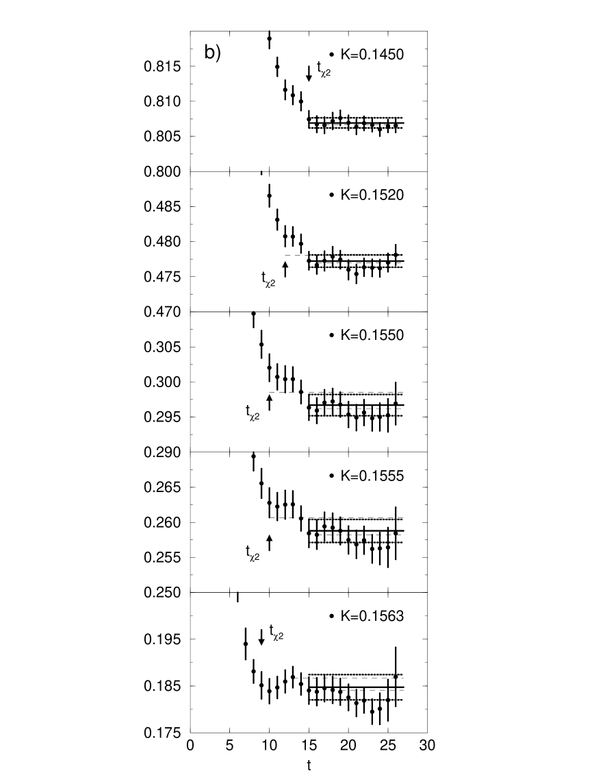
Figure 6: Effective masses for the pion: a) $\beta=5.85$, b) $\beta=6.0$. The result of one-mass fit is reproduced by the solid line, dotted lines and dashed lines for the fitted mass, its statistical error and systematic upper/lower bounds, respectively.

We show $m_{\it eff}$ at $\beta=5.85$ and $\beta=6.0$ in Fig. 6. The pion effective mass has structure with the scale of the standard deviation even for $t\geq t_{\chi^{2}}$: In some cases $m_{\it eff}(t)$ exhibits two-plateau structure or slow monotonic decrease. However, the magnitude of the fluctuation for the pion is much smaller than the other cases. The resulting systematic error is comparable to the statistical uncertainty. The results of the fits are given in table 3.

3.4 Rho meson masses

Fitting to the $\rho$ meson propagator is more problematic than the pion propagator. Because of this, we will discuss it at some length and compare the results with previous works.

The $\rho$ meson effective mass at $\beta=5.85$ shown in Fig. 7-a exhibits a plateau for $t\geq t_{\chi^{2}}=12$ for the smallest two $K$’s, while it exhibits peculiar behavior at large $t$ for the largest three $K$’s: $m_{\it eff}(t)$ for $t=17$ — 20 is larger than that for $t=12$ — 16 and it drops abruptly at $t=21$. We regard this behavior as due to statistical fluctuations. We find that fits to a range $t=12$ — $t_{max}$ are stable for $t_{max}=$ 14 — 27. Therefore we choose $t_{max}=T/2$ even for these cases. The results of the fits are summarized in table 4. The systematic error upper bound is 1 — 2 times larger than the statistical error for the largest three $K$’s.

Fig. 7-b shows the effective mass at $\beta=6.0$. Except for the smallest $K$, $m_{\it eff}(t)$ is decreasing at $t\sim t_{\chi^{2}}$. Rate of the decrease becomes slow at $t\sim 12$ to exhibit a plateau for two or three time slices. The value of $m_{\it eff}$ decreases further up to $t\sim 17$ to attain another plateau. The plateaus are not long enough to determine unambiguously the time slice where the contribution of excited states can be ignored. It should be emphasized again that $\chi^{2}/df$ are almost identical both for the fits with $t_{min}=12$ and $t_{min}=17$: 1.35 and 1.16 for $K=0.1550$, 1.20 and 1.13 for $K=0.1555$ and 0.77 and 0.76 for $K=0.1563$, respectively. See also Fig. 4. Therefore the value of $\chi^{2}$ does not give a guide to determine $t_{min}$. The point $t_{min}=15$ is located between the two pseudo-plateaus at $t\sim 12$ and $t\sim 17$. In table 4 are summarized the results for the fits with $t_{min}=15$ together with the systematic error. Reflecting the slow monotonic decrease of effective masses, the ratio of the systematic error to the statistical error is relatively large: the systematic error amounts to about twice the statistical error for the largest three $K$’s.

We notice a very intriguing fact that $m_{fit}$ by the correlated fits to a range from $t=t_{0}$ to $T/2$ has a strong correlation with $m_{\it eff}$ at $t=t_{0}$. A typical example is seen in Fig. 4. This holds for the other particles also. This means that the result of the fit to a range $t_{0}$ — $T/2$ is mainly determined from data at $t\sim t_{0}$.

In our previous work [4], we analyzed the same set of $\rho$ meson propagators with uncorrelated fits. Paying attention to the monotonic decrease of effective masses, we made two different fits to estimate the systematic error coming from uncertainties in the choice of fitting range. One is a fit to a range $t\sim$ 9 — 11 at $\beta=5.85$ ($t\sim$ 12 — 15 at $\beta=6.0$). We called the fit “pre-plateau fit”. Another is a fit to a range $t\sim$ 11 — $t_{max}$ at $\beta=5.85$ ($t\sim$ 15 — $t_{max}$ at $\beta=6.0$), which we called “plateau fit”. The latter fitting ranges correspond approximately to those we adopt in this work. Because $m_{\it eff}$ is decreasing, the $\rho$ masses obtained from the correlated fits are systematically larger than those from the uncorrelated fits, due to the fact give in the preceding paragraph. The mass value obtained in this work is between that from the uncorrelated plateau fit and that from the pre-plateau fit.

In table 5 we reproduce the results for the $\rho$ meson masses at $\beta=6.0$ for $K=0.155$ and 0.1563 together with those by the Ape collaboration [6, 7] and the LANL group [11]. In 1991, the Ape collaboration reported the result obtained on a $24^{3}\times 32$ lattice with a multi-origin $7^{3}$ cubic source [7]. Then we made simulations for the same spatial size with larger temporal extent [4], $24^{3}\times 54$, using the point source. For $K=0.155$, the values of $m_{\it eff}$ at $t\sim 10$ are in close agreement with Ape’s. Consequently the result 0.4280(33) obtained from the pre-plateau fit ($t=$ 12 — 15) agreed with the Ape result 0.429(3) within one standard deviation. However, the result 0.4169(48) from the plateau fit ($t=$ 15 — 27) was smaller by approximately twice the statistical error. We regarded the latter more reliable. At that time there was a report that the mass value appears to depend on the type of the source adopted [13]. Therefore, in order to clarify whether the origin of the discrepancy between our result and the Ape result is due to the different type of source, we made calculation at $K=0.155$ for 400 configurations [5] using the point source, the wall source and the source adopted by the Ape collaboration. The results obtained from correlated fits for the three different sources have agreed with each other; 0.4201(29), 0.4228(19) and 0.4249(19) for the point source, the wall source and the multi-origin source, respectively. The recent result reported by the LANL group 0.422(3) [11] is consistent with these numbers. It is probable that the slightly large value by the Ape collaboration is due to small temporal extent. The Ape collaboration has also made simulations using both the point source and the multi-cube source [6] with larger temporal size and smaller spatial size: $18^{3}\times 64$. Their results 0.430(10) and 0.428(8) are consistent with other results within relatively large errors, although the central values are slightly higher than the results by other groups. The slightly large central values may be due to the small spatial size. For $K=0.1563$, the results obtained from the correlated fit in this work is consistent with those by the Ape collaboration and the LANL group, albeit with large errors in the results.

3.5 Baryon masses

Fig. 8 shows effective masses for the nucleon at $\beta=5.85$ and $\beta=6.0$. Decrease of $m_{\it eff}$ at $t\sim t_{\chi^{2}}$ is not conspicuous compared with the case of the $\rho$ meson. However, we see two-plateau structure for the cases of $K=0.1585$ and 0.1595 at $\beta=5.85$ and $K=0.155$ (see also Fig. 5) and 0.1555 at $\beta=6.0$. The choice $t_{min}=13\ (16)$ for $\beta=5.85\ (6.0)$ corresponds to that we select the first (last) plateau as correct for the case where two plateaus are observed. Table 6 summarizes the results of the fits.

For $\Delta$, monotonic decrease of effective masses at $t\sim t_{\chi^{2}}$ or two-plateau structure is seen for $K=0.1595$ and 0.1605 at $\beta=5.85$ and for $K=0.1550$ and 0.1563 at $\beta=6.0$. Effective mass plots are shown in Fig. 9. The results of the fits are summarized in table 7.

In table 5, the baryon masses at $\beta=6.0$ for $K=0.155$ and 0.1563 together with those by the Ape collaboration and the LANL group are reproduced. The nucleon masses reported by the three groups agree within the statistical uncertainties. The $\Delta$ masses for $K=0.155$ are slightly scattered: Our result is higher than the LANL result by two standard deviations. However note that the values of the $\Delta$ mass obtained on 400 configurations [5] (0.7054(95), 0.7008(57) and 0.7128(191) for the point source, the wall source and the multi-origin source, respectively) are in good agreement with the LANL result. Therefore we think that the difference between the LANL result and our present result is due to statistical errors.

3.6 Finite lattice effects

The linear extension of the lattice in the spatial directions is 2.45 (2.03) fm at $\beta$ = 5.85 (6.0), when we use $a^{-1}=1.93$ (2.33) GeV determined from $m_{\rho}$ (see Sec. 5). These values are much larger than twice the electromagnetic radius of the nucleon, $2\times$ 0.82 fm. We also note that our results on the lattice with spatial volume $24^{3}$ agree well with those on a lattice with $32^{3}$ [11], as discussed above. Therefore we do not take into account in this work finite lattice effects which are supposed to be small.

3.7 Mass ratios

The mass ratio $m_{N}/m_{\rho}$ is plotted versus $(m_{\pi}/m_{\rho})^{2}$ in Fig. 10. The values of the mass ratio are given in table 8. The value of $m_{N}/m_{\rho}$ at $\beta=6.0$ is systematically smaller than that at $\beta=5.85$, although the results at two $\beta$’s agree within the statistical uncertainty except for the case of the heaviest quark (($m_{\pi}/m_{\rho})^{2}\sim 0.94$).

4 Excited State Masses

In addition to the masses of ground states, we study the masses of first excited states for the $\rho$ meson and the nucleon. To this end, we perform two-mass fits to the corresponding propagators varying $t_{min}$. Our results for the $\rho$ meson are shown in Fig. 11 for $\beta=5.85$, $K=0.1585$, and in Fig. 12 for $\beta=6.0$, $K=0.155$. The results for the nucleon are given in Figs. 13 and 14 for $\beta=5.85$ and 6.0, respectively. We find the following:

1) $\chi^{2}/df$ is stable and small ($\sim 1$ — 2) for $t_{min}\geq 4\ (5)$ in the case of the $\rho$ meson and for $t_{min}\geq 5\ (6)$ in the case of the nucleon at $\beta=5.85\ (6.0)$, respectively.

2) When $\chi^{2}/df$ is small, the ground state masses $m_{0}$ from the two-mass fit are consistent with those from the one-mass fit within the errors, although the errors for $m_{0}$ from the two-mass fit become extremely large at large $t_{min}$.

3) Although $\chi^{2}/df$ is stable, the mass of the first excited state $m_{1}$ is in general quite unstable. For example, for the $\rho$ meson at $\beta=5.85$, the value of $m_{1}$ decreases from 1.5 for $t_{min}=3$ to 0.6 for $t_{min}=9$ (cf. Fig. 11). Similar behavior is also seen in the results for the $\rho$ meson at $\beta=6.0$ (Fig. 12) and the nucleon at $\beta=5.85$ (Fig. 13). The case of the nucleon at $\beta=6.0$ is exceptional: $m_{1}$ is relatively stable (Fig. 14).

Under these circumstances, we select two $t_{min}$’s which give $m_{0}$ consistent with the result of the one-mass fit, under the condition that the errors are small. We then investigate whether the results for the excited state mass are consistent with the corresponding experimental values.

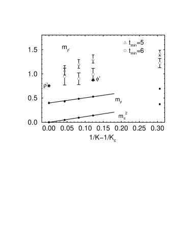
Figure 15: Mass of the excited state of the $\rho$ meson (denoted by $\rho^{\prime}$) at $\beta=5.85$ versus $1/K-1/K_{c}$. The corresponding experimental values are marked with stars. The data for $m_{\rho}$ and $m_{\pi}^{2}$ are taken from the results of one-mass fits. With the scale of the plot, the results for $m_{\rho}$ from two-mass fits are indistinguishable from the one-mass fit results.

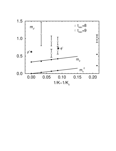
Figure 16: The same as Fig. 15 for $\beta=6.0$.

In Figs. 15 and 16 are shown the first excited state masses of the $\rho$ meson obtained from the fit with $t_{min}=5$ and 6 (8 and 9) versus $1/K$ at $\beta=5.85\ (6.0)$, respectively. (A two-mass fit with $t_{min}=9$ for the largest $K$ at $\beta=6.0$ does not converge. Therefore the corresponding data is missing in the figure.) We give in the figures the experimental values for the masses of $\rho(1450)$ and $\phi(1680)$ which are the first excited states of the vector mesons. The mass of $\phi(1680)$ is plotted at the third largest $K$, because this value of $K$ corresponds to the strange quark mass as mentioned in Sec. 5.7. Apparently the results for the excited state mass depend strongly on the value of $t_{min}$. For quarks lighter than the strange quark, the excited state mass obtained with smaller $t_{min}$ is much larger than experiment, while that with larger one is consistent with experiment within large statistical errors. Therefore, although the value of $m_{1}$ is unstable, there exist two-mass fits to the $\rho$ propagators which give both the ground state mass consistent with the one-mass fit and the first excited state mass consistent with experiment.

Fig. 17 shows the masses of excited state of the nucleon at $\beta=5.85$ versus $1/K$. The excited state masses obtained from the fit with $t_{min}=7$ are much smaller than those with $t_{min}=6$. (A two-mass fit with $t_{min}=7$ for the largest $K$ does not converge.) We expect that the mass difference between the ground state and the first excited state depends only weakly on the quark mass, because the mass difference for the spin $1/2$ baryon satisfies this property. The mass difference for the nucleon is $m_{N(1440)}-m_{N(940)}=500$ MeV. The figure shows that the excited state masses with $t_{min}=7$ lie approximately 500 MeV higher than the ground state masses. Therefore there exist two-mass fits whose results do not contradict with experiment also for the nucleon at $\beta=5.85$.

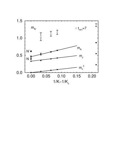
Figure 18: The same as Fig. 17 for $\beta=6.0$.

In Fig. 18 we show the excited state masses of the nucleon at $\beta=6.0$ with $t_{min}=7$. The masses of the first excited state lie much more than 500 MeV above the ground state masses. As mentioned before, two-mass fits for the nucleon at $\beta=6.0$ are stable and therefore the values of the excited state mass do not change much even if we take other $t_{min}$. When we recall that there exists a fit which gives a reasonable excited state mass at $\beta=5.85$, this situation is puzzling. One possible origin for the heavy excited state mass at $\beta=6.0$ is a finite size effect, because the physical volume is smaller at $\beta=6.0$. There remains a possibility that when we simulate on a larger lattice, a two-mass fit with larger $t_{min}$ gives a value consistent with the nucleon excited state mass.

There are several published data for the mass of excited states [5, 7, 8, 22, 23]. In table 9, we reproduce the results for the ratio of the excited state mass to the ground state mass selecting the quark mass corresponding approximately to the strange quark mass. For the $\rho$ meson, except our results in this work with $t_{min}=6$ (9) at $\beta=5.85$ (6.0) and the result for the wall source in ref. [5], the reported ratios are considerably larger than the corresponding experimental value $m_{\phi(1680)}/m_{\phi(1020)}=1.65$. For the nucleon, the mass ratios reported by the Ape collaboration and the UKQCD collaboration are considerably larger than our result. One possible origin of the differences is due to the choice of fitting range. Because the two-mass fit is very unstable, we certainly have to employ a more efficient way to extract reliable values for the excited state masses.

5 Masses of Hadrons with Physical Light Quarks

5.1 Extrapolation procedure

Extrapolation of hadron masses to the chiral limit is done with the correlation being taken into account, among the masses at different values of hopping parameter. First we consider a least mean square fit to minimize

$$\chi^{2}=\sum_{t,t^{\prime},K,K^{\prime}}\{G(t,K)-G_{0}(t,K)\}\,C^{-1}(t,K;t^{\prime},K^{\prime})\,\{G(t^{\prime},K^{\prime})-G_{0}(t^{\prime},K^{\prime})\},$$ (14)

where $G_{0}(t,K)=A(K)e^{-m(K)t}$ is the fitting function to hadron propagator $G(t,K)$ and $C^{-1}$ is the inverse of the full correlation matrix $C(t,K;t^{\prime};K^{\prime})$. A linear approximation to the fitting function around the minimum of $\chi^{2}$ gives the relation between the error matrix $\Sigma$ for fit parameters and correlation matrix $C(t,K;t^{\prime},K^{\prime})$ for propagators:

$$\Sigma=(D^{T}C^{-1}D)^{-1},$$ (15)

where $D$ is the Jacobian defined by

$$D_{t,K;A(K^{\prime}),m(K^{\prime})}=[{\partial G_{0}(t,K)}/{\partial A(K^{\prime})},{\partial G_{0}(t,K)}/{\partial m(K^{\prime})}].$$ (16)

($D$ is diagonal with respect to $K$.) The full least mean square fit to minimize $\chi^{2}$ in eq. 14 is different from the set of least mean square fits for each $K$ to minimize $\chi^{2}$’s in eq. 12: The masses and amplitudes obtained by the two methods are in general different. We take those obtained from the fits to each propagator for evaluation of the Jacobian.

For extrapolation, we minimize $\chi^{2}$ given by

$$\chi^{2}=\sum_{K}\{m(K)-f(K)\}\,\Sigma^{-1}(K,K^{\prime})\,\{m(K^{\prime})-f(K^{\prime})\},$$ (17)

where the correlation matrix $\Sigma(K,K^{\prime})$ is the sub-matrix among the masses of the full error matrix $\Sigma$ and $f(K)$ is the fitting function. (For the pion, $m(K)$ is replaced by $m^{2}(K)$ with appropriate replacement of $\Sigma^{-1}(K,K^{\prime})$.)

5.2 Linear extrapolation to the chiral limit

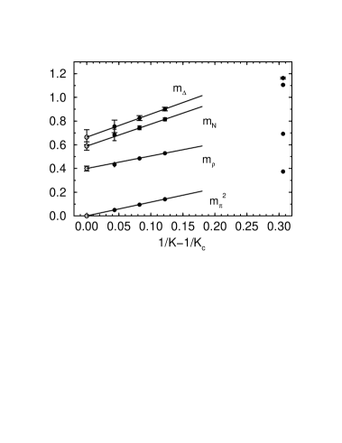
Figure 19: Linear extrapolations of hadron masses at $\beta=5.85$ to the chiral limit. The open circles at zero quark mass are extrapolated values. The errors shown are statistical only, and do not include the systematic errors discussed in the text.

We fit the data of the mass squared for the pion and the mass for the other hadrons at the largest three $K$’s to a linear function of $1/K$; $f(K)=a_{0}+a_{1}/K$. We find that quality of the linear fit is good in the sense that $\chi^{2}/df<2$ ($df=1$ in this case) and therefore we do not study in this work the effects of possible chiral logarithms [24, 25]. We summarize the fit parameters together with $\chi^{2}/df$ in table 10. The linear extrapolations of hadron masses at $\beta=5.85$ and 6.0 are shown in Figs. 19 and 20, respectively.

In table 11 we summarize the results for the critical hopping parameter $K_{c}$ and the masses at $K_{c}$ together with the errors estimated by the least mean square fit and those by the jack-knife method. We find that the error estimated by the jack-knife method is larger than that by the least mean square fit except for $K_{c}$ at $\beta=6.0$. We take the error obtained by the jack-knife method as our estimate of the statistical uncertainty, unless otherwise stated.

5.3 Systematic error analyses

We first estimate the systematic error on the masses in the chiral limit coming from uncertainties in the choice of fitting range for extracting the ground state mass at each $K$. To this end, we repeat linear extrapolations of the masses obtained from the fits to a range $t_{0}$ — $T/2$, varying $t_{0}$ (common to all $K$’s) from ${\rm max}_{K}\{t_{\chi^{2}}(K)\}$ to $t_{min}+4$. We find that quality of the linear fits depends on the choice of $t_{0}$: $\chi^{2}/df$ are considerably large for some choices of $t_{0}$. We adopt the condition $\chi^{2}/df<2$ for the linear fit to be accepted. We take the difference between the fitted mass value and the maximum/minimum mass value under the condition $\chi^{2}/df<2$ as our estimate of the systematic upper/lower error. We call the systematic error thus obtained the fit-range systematic error.

Data at the fourth largest $K$ slightly deviates from the linear fit. In order to estimate the systematic error which comes from the choice of fitting function, we make a quadratic fit ($f(K)=a_{0}+a_{1}/K+a_{2}/K^{2}$) to the largest four $K$’s, varying $t_{0}$ in the range used for the estimate of the fit-range systematic error. We estimate the systematic error by the difference between the maximum/minimum value with $\chi^{2}/df<2$ and that of the linear fits. We call the systematic error thus obtained the fit-func systematic error.

5.4 Pion mass extrapolation and $K_{c}$

Pion masses squared are fitted to a linear function of $1/K$ to obtain the critical hopping parameter. The value of $\chi^{2}/df$ is 0.56 (1.1) for the fit ($t_{min}=12$ (15)) at $\beta=5.85$ (6.0). The fit-range systematic errors are estimated from the fits with $t_{0}=8$ — 16 at $\beta=5.85$ and 10 — 19 at $\beta=6.0$. All the fits give $\chi^{2}/df<2$. The upper (lower) bound comes from the fit with $t_{0}=11$ (14) with $\chi^{2}/df$ of 0.36 (0.04) for $\beta=5.85$ and from the fit with $t_{0}=12$ (19) with $\chi^{2}/df$ of 0.44 (0.96) for $\beta=6.0$.

For data at $\beta=5.85$, no quadratic fits with $t_{0}=8$ — 16 give $\chi^{2}/df<2$. On the other hand, quadratic fits to data at $\beta=6.0$ with $t_{0}=13$ — 19 give $\chi^{2}/df<2$. Because $m_{\pi}^{2}$ is a concave function of $1/K$ when the data at the fourth largest $K$ is included, $K_{c}$ obtained from the quadratic fit is larger than that from the linear fit.

The values of $K_{c}$’s together with the fit-range systematic error and the fit-func systematic error are given by

		stat.	sys.(fit-range)		sys.(fit-func.)
$\beta=5.85$	$K_{c}=$ 0.161624	$\pm$0.000033	+0.000001	$-$0.000025
$\beta=6.00$	$K_{c}=$ 0.157096	$\pm$0.000028	+0.000033	$-$0.000009	+0.000109

The fit-range systematic error is comparable to the statistical uncertainty.

The result for $K_{c}$ at $\beta=6.0$ agrees well with that in ref. [7]. Although it is slightly smaller than the LANL result 0.15714(1) [11], we conclude that our result is consistent with theirs within the sum of the statistical error and the fit-range systematic error.

In this work, we do not distinguish the physical point where $m_{\pi}/m_{\rho}$ takes its experimental value from the critical point where the pion mass vanishes, because we find that physical quantities at the two points differ only at most 30% of their statistical errors.

5.5 Rho meson mass extrapolation and lattice spacing

A linear fit to the $\rho$ meson masses (with $t_{min}=12$ (15)) at the largest three $K$’s gives $\chi^{2}/df$ of 1.8 (1.2) for $\beta=5.85$ (6.0). Therefore the linear fit is acceptable.

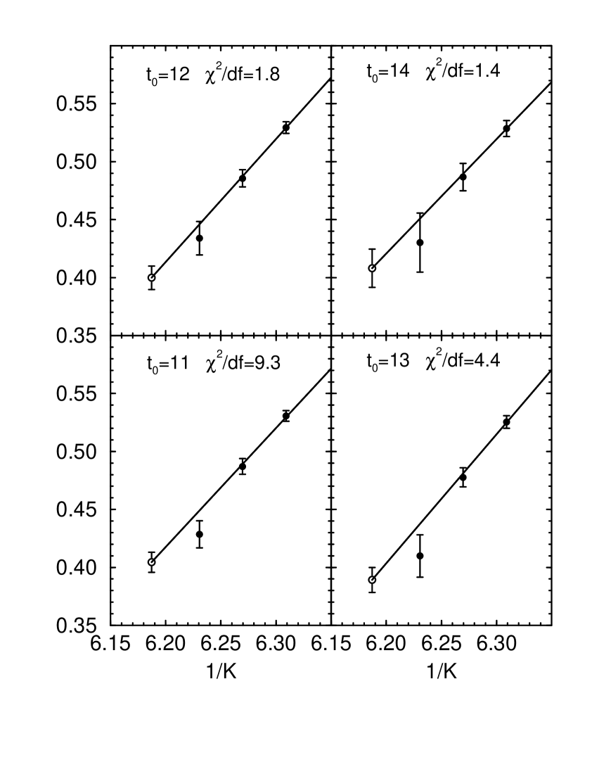
Figure 21: $\rho$ meson masses at $\beta=5.85$ obtained from the fit with various $t_{0}$ together with linear extrapolations of these data. The open circles are extrapolated values. The errors shown are those estimated by the least mean square fits.

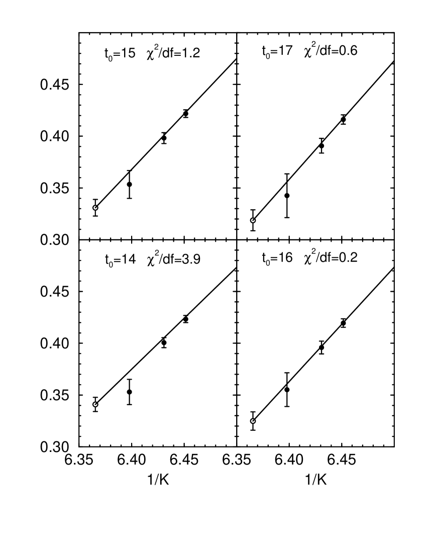
Figure 22: The same as Fig. 21 but for $\beta=6.0$.

However, we find that quality of the linear fit strongly depends on the choice of fitting range. See Figs. 21 and 22. In table 12, we summarize $\chi^{2}/df$, $m_{\rho}(K_{c})$ and the inverse lattice spacing defined by $a^{-1}=0.77{\rm GeV}/m_{\rho}(K_{c})$ versus $t_{0}$.

We also make a quadratic fit to the data at the largest four $K$’s to estimate the systematic error due to the choice of fitting function. Table 13 summarizes the results of the quadratic fits versus $t_{0}$.

The method to estimate the systematic error is the same as that adopted for the pion. Our final results for $m_{\rho}$ are

		stat.	sys.(fit-range)		sys.(fit-func.)
$\beta=5.85$	$m_{\rho}(K_{c})$ = 0.400	$\pm$0.021	+0.008	$-$0.027	+0.0	$-$0.013
$\beta=6.00$	$m_{\rho}(K_{c})$ = 0.331	$\pm$0.011	+0.018	$-$0.020	+0.0	$-$0.008

The value of $m_{\rho}(K_{c})$ at $\beta=6.0$ agrees well with the Ape result 0.3332(75) and the LANL result 0.3328(106). The values of $m_{\rho}(K_{c})$’s are translated to the lattice spacing as

		stat.	sys.(fit-range)		sys.(fit-func.)
$\beta=5.85$	$a^{-1}=$ 1.93	$\pm$0.10	+0.14	$-$0.04	+0.08	$-$0.0     GeV
$\beta=6.00$	$a^{-1}=$ 2.33	$\pm$0.08	+0.15	$-$0.12	+0.06	$-$0.0     GeV

Although the statistical error on $a^{-1}$ is several percent, we notice that the systematic error is much larger. Summing up both the statistical and systematic errors, we find that $a^{-1}$ can be as large as 2.25 GeV (2.62 GeV) at $\beta=5.85\ (6.0)$ and as small as 1.79 GeV (2.13 GeV).

In analyses of the systematic errors above, we have taken $t_{0}$ common to all $K$’s. However, it is not necessary to restrict ourselves to take a common value of $t_{0}$, because the time slice at which the contribution of excited states becomes negligible can depend on the quark mass. We make linear fits to all possible combinations of the $\rho$ masses at the largest three $K$’s, varying $t_{0}$ separately for each $K$ from $t_{\chi^{2}}$ to 18. Fig. 23 shows $a^{-1}$ at $\beta=6.0$ versus $\chi^{2}/df$. We see that there are linear fits with small $\chi^{2}/df$ which give both large and small $a^{-1}$. The value of $a^{-1}$ scatters approximately from 2.15 GeV to 2.65 GeV. This upper value as well as the lower value are consistent with those obtained above with the systematic errors included.

We estimate the value of $J$ defined by $m_{V}{{dm_{V}}\over{dm_{PS}^{2}}}$ [23] from the linear fits discussed above:

		stat.	sys.(fit-range)
$\beta=5.85$	$J=$ 0.420	$\pm$0.049	+0.028	$-$0.024
$\beta=6.00$	$J=$ 0.395	$\pm$0.026	+0.026	$-$0.026

The value of $J$ at $\beta=6.0$ is smaller than the experimental value 0.48(2) even when we include the systematic errors.

5.6 Nucleon and $\Delta$ masses

Both linear fits and quadratic fits are made to the masses of the nucleon and the $\Delta$ baryon by the same method as for the $\rho$ meson. Results of the linear fits versus the fit-range are summarized in tables 14 and 15. The fit with $t_{min}=13\ (16)$ at $\beta=5.85$ (6.0), which is adopted in this work, gives a small $\chi^{2}/df=$ 0.37 (0.05). For the nucleon, quality of the linear fits is good for almost all values of $t_{0}$ in the sense that $\chi^{2}/df$ are approximately less than 2, except for the fit with $t_{0}=9$ at $\beta=5.85$. This feature is different from that for the $\rho$ meson. Quality of the fits to the $\Delta$ masses at $\beta=5.85$ is good for $t_{0}\leq 13$ including our choice $t_{min}=13$ and that at $\beta=6.0$ is good for all $t_{0}$ except for $t_{0}=13$.

Results with various errors are give by

		stat.	sys.(fit-range)		sys(fit-func.)
$\beta=5.85$	$m_{N}(K_{c})=$ 0.589	$\pm$0.036	+0.018	$-$0.058	+0.0	$-$0.018
$\beta=6.00$	$m_{N}(K_{c})=$ 0.462	$\pm$0.024	+0.020	$-$0.009	+0.0	$-$0.007

		stat.	sys.(fit-range)		sys.(fit-func.)
$\beta=5.85$	$m_{\Delta}(K_{c})=$ 0.664	$\pm$0.063	+0.034	$-$0.0	+0.0	$-$0.031
$\beta=6.00$	$m_{\Delta}(K_{c})=$ 0.605	$\pm$0.033	+0.041	$-$0.011	+0.016	$-$0.007

The value of the nucleon mass in the chiral limit at $\beta=6.0$ lies between the LANL result 0.482(13) and the Ape result 0.432(15). For the $\Delta$ masses, results by the three groups agree well with each other, albeit with large errors; the LANL result is 0.590(30) and the Ape result 0.58(3). The LANL results are those at the physical point where $m_{\pi}/m_{\rho}$ takes its experimental value.

These results are translated to the masses in physical units using the value of $a^{-1}$ obtained from $m_{\rho}$. The systematic error on the lattice spacing is not taken into account for the estimate of the systematic error on the baryon masses. Results read

		stat.	sys.(fit-range)		sys.(fit-func.)
$\beta=5.85$	$m_{N}=$ 1.135	$\pm$0.088	+0.034	$-$0.112	+0.0	$-$0.034      GeV
$\beta=6.00$	$m_{N}=$ 1.076	$\pm$0.060	+0.047	$-$0.020	+0.0	$-$0.017      GeV
$\beta=5.85$	$m_{\Delta}=$ 1.279	$\pm$0.136	+0.066	$-$0.0	+0.0	$-$0.059      GeV
$\beta=6.00$	$m_{\Delta}=$ 1.407	$\pm$0.086	+0.096	$-$0.026	+0.038	$-$0.015      GeV

The central value of the nucleon mass at $\beta=6.0$ (5.85) is larger than its experimental value by about 15% (20%) and that of the $\Delta$ mass by about 15% (4%): The errors amount to twice the statistical errors except for the $\Delta$ baryon at $\beta=5.85$. The systematic errors are comparable with the statistical errors (3 — 13%). Even when the systematic errors are included, the baryon masses at $\beta=6.0$ do not agree with experiment. Our data are consistent with the GF11 data [10] at finite lattice spacing, within statistical errors. In order to take the continuum limit of our results, we need data for a wider range of $\beta$ with statistical and systematic errors much reduced.

5.7 Masses of strange hadrons

The hopping parameters for the strange quark which are estimated from the experimental value of $m_{K}/m_{\rho}$ turn out to be $K_{s}=0.1588$ and 0.1550 at $\beta=5.85$ and 6.0, respectively. Note that they are identical or almost identical to the third largest hopping parameter $K=0.1585$ and 0.1550 which we have chosen in such a way that they approximately correspond to the strange quark. The masses of $\Omega^{-}$ estimated at $K=K_{s}$ are 1.696(92) GeV and 1.693(57) GeV at $\beta=5.85$ and 6.0, respectively (statistical errors only). They are in good agreement with the experimental value 1.672 GeV. The masses of the vector meson at $K=K_{s}$ are 998(45) MeV and 986(26) MeV at $\beta=5.85$ and 6.0, respectively, which equal the $\phi$ meson mass 1019 MeV within about one standard deviation. As is well known, there are ambiguities in determination of the hopping parameter for the strange quark. When the hopping parameters for the strange quark mass are alternatively determined from $m_{\phi}/m_{\rho}$, they are equal to $0.1585$ and 0.1547. The results for the $\Omega^{-}$ mass at these hopping parameters are consistent with those above within one standard deviation.

6 Meson Decay Constants

6.1 Vector meson decay constants

We evaluate vector meson decay constants defined by

$$\langle 0|(\bar{u}\gamma_{i}d)^{cont.}|V({\vec{p}}=0)\rangle=\epsilon_{i}F_{V}m_{V},$$ (18)

where $\epsilon_{i}$ and $m_{V}$ are the polarization vector and the mass of the vector meson, respectively, and $(\bar{u}\gamma_{i}d)^{cont.}$ is the vector current in the continuum limit. The experimental value for the $\rho$ meson is $F_{\rho}=216(5)$ MeV. (This $F_{V}$ is related to $f_{V}^{-1}$ by $f_{V}^{-1}=F_{V}/m_{V}$.)

The expectation value of the local lattice current $(\bar{u}\gamma_{i}d)^{latt.}$ between the vacuum and the vector meson is related to the continuum one by the relation

$$\langle 0|(\bar{u}\gamma_{i}d)^{cont.}|V({\vec{p}}=0)\rangle=Z_{K}Z_{V}\langle 0|(\bar{u}\gamma_{i}d)^{latt.}|V({\vec{p}}=0)\rangle.$$ (19)

The coefficient $Z_{K}$ is a scale factor for the difference between the continuum and lattice normalizations of the quark field. The renormalization constant $Z_{V}$ is the ratio of the conserved lattice current to the local current, which can be estimated by perturbation theory or numerical simulations. We test the following three possible choices of $Z_{K}$ and $Z_{V}$:

1. those in naive perturbation theory: $Z_{K}=2K$ and $Z_{V}=1-0.174\,g^{2}$ [16],

2. those in tadpole improved perturbation theory: $Z_{K}=(1-3K/4K_{c})$ [17] and $Z_{V}=1-0.82\,\alpha_{\overline{MS}}(1/a)$ [18]   ($\alpha_{\overline{MS}}(\pi/a)=g^{2}_{\overline{MS}}(\pi/a)/4\pi$ is determined by the relation $1/g^{2}_{\overline{MS}}(\pi/a)={\rm Tr}(U_{P}/3)/g^{2}+0.02461$  [18, 19]. We then determine $\alpha_{\overline{MS}}(1/a)$ using the two loop renormalization group equation.),

3. Monte Carlo estimate of $Z_{V}$ = 0.51 [2] (0.57 [20]) at $\beta=5.85\ (6.0)$ with $Z_{K}=2K$. (Data for $Z_{V}$ at $\beta=5.85$ [2] are given in table 16. Because the results for $Z_{V}$ are independent of the quark mass in the range we investigate, we use the averaged value.) The error on $Z_{V}$ is ignored in the following.

We abbreviate the decay constants obtained using the above three renormalization constants as $F_{V}^{PT}\ F_{V}^{TP}$ and $F_{V}^{MC}$, respectively.

The statistical error is obtained by the jack-knife method. The systematic error is estimated varying $t_{0}$ as in the case of mass calculation. The range of $t_{0}$ is the same as that for the $\rho$ mass. In table 17 we summarize the results for the decay constants at each $K$. We quote the error only for $F_{V}^{TP}$, because the errors for the others can be easily obtained from that for $F_{V}^{TP}$ by multiplying the ratio of $Z$-factors.

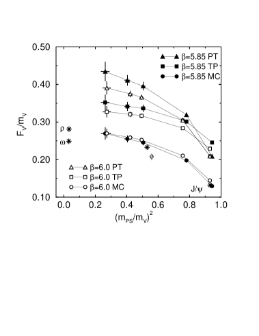
Figure 24: Ratio of the vector meson decay constant to the vector meson mass, for the three choices of renormalization constants discussed in the text. The errors shown are statistical only and are estimated by the jack-knife method. The corresponding experimental values for vector mesons are marked with stars. The value of $m_{PS}$ for the strange quark is estimated by phenomenological mass formulae[15] using $m_{V}=m_{\phi}=1019$ MeV.

Fig. 24 shows $F_{V}/m_{V}$ versus $(m_{PS}/m_{V})^{2}$ together with the corresponding experimental values for $\rho$, $\omega$, $\phi$ and $J/\psi$. Note that we can compare the numerical results with the experimental values for $\phi$ and $J/\psi$ without extrapolation. The values with $F_{V}^{MC}$ at two $\beta$’s remarkably agree with each other. Furthermore they agree well with the experimental values for $\phi$ and $J/\psi$. This implies that scaling violation in $F_{V}^{MC}$ is small. On the other hand, we find sizable scaling violation in $F_{V}^{PT}$ and $F_{V}^{TP}$. They are off the experimental values for $\phi$ and $J/\psi$ by 40 — 100%. We find that $F_{V}^{MC}/m_{V}$’s at $\beta=6.0$ agree well with the Ape data [7, 8].

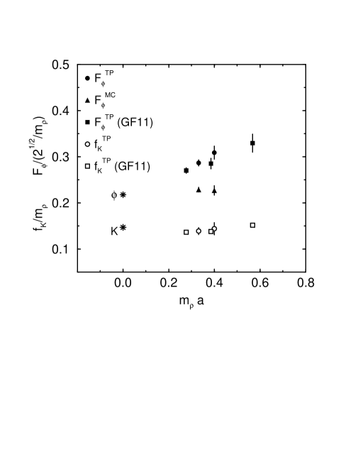
Figure 25: Ratios of the $\phi$ meson decay constant and the $K$ meson decay constant to the $\rho$ meson mass versus the $\rho$ meson mass in lattice units. The errors in our data are statistical only. The GF11 data are taken from ref. [21]. The corresponding experimental values are marked with stars.

In fig. 25 we depict the values of $F_{\phi}/m_{\rho}$ versus $m_{\rho}a$ together with the GF11 result[21]. The values of the hopping parameter for the strange quark are given in Sec. 5.7. Note that the values of $F_{\phi}^{MC}/{m_{\rho}}$ agree with experiment already at $m_{\rho}a$ = 0.33 — 0.40 within 1 — 2 standard deviations. The values of $F_{\phi}^{TP}/{m_{\rho}}$ are consistent with the GF11 result, although the central values are about $1\sigma$ higher than the GF11 data. They are off the experimental value by 30 — 40% at these values of $m_{\rho}a$. Linear extrapolation of our data to zero lattice spacing is consistent with experiment.

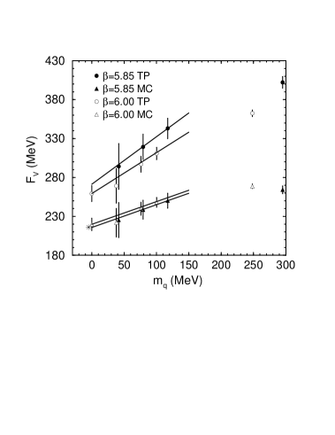
Figure 26: Linear extrapolations of vector meson decay constants, for the two choices of renormalization constants discussed in the text. The open symbols at zero quark mass are extrapolated values for $\beta=6.0$. The errors shown are statistical only. The experimental value for the $\rho$ meson is marked with a star.

The value of $F_{V}$ in the chiral limit is obtained from a linear fit in terms of $1/K$ in a similar way to that made for hadron mass extrapolation. We first calculate the correlation matrix $\Sigma(K,K^{\prime})$ for $F_{V}(K)$ from the error matrix $\Sigma$ for the mass and amplitude (eq. 15) using the error propagation rule and then minimize $\chi^{2}$. A linear fit to the data at the largest three $K$’s gives a reasonable $\chi^{2}/df$: $\chi^{2}/df$ = 0.04 (0.38) for $F_{V}^{TP}$, 0.09 (0.44) for $F_{V}^{PT}$ and $F_{V}^{MC}$ at $\beta=5.85$ (6.0), respectively. Fig. 26 shows $F_{V}$ as functions of the quark mass together with the fitting functions.

The method to estimate the systematic error due to the choice of fitting range is similar to that for hadron masses at $K_{c}$. The results of the linear fit for various fitting ranges are given in table 18. Our final results for $F_{\rho}$ read

		stat.	sys.(fit-range)
$\beta=$ 5.85	$F_{\rho}^{TP}=$ 0.141	$\pm$0.017	+0.007	$-$0.035
	$F_{\rho}^{TP}=$ 271	$\pm$20	+14	$-$68	MeV
	$F_{\rho}^{MC}=$ 0.112	$\pm$0.013	+0.006	$-$0.027
	$F_{\rho}^{MC}=$ 216	$\pm$15	+11	$-$52	MeV
$\beta=$ 6.00	$F_{\rho}^{TP}=$ 0.111	$\pm$0.008	+0.016	$-$0.017
	$F_{\rho}^{TP}=$ 259	$\pm$10	+37	$-$40	MeV
	$F_{\rho}^{MC}=$ 0.0944	$\pm$0.0064	+0.010	$-$0.014
	$F_{\rho}^{MC}=$ 220	$\pm$8	+24	$-$33	MeV

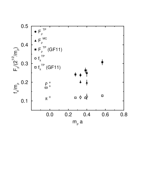
Figure 27: The same as Fig. 25 for the $\rho$ meson and the pion.

The values of $F_{\rho}^{PT}$ can be obtained from $F_{\rho}^{MC}$ by multiplying $Z_{V}^{PT}/Z_{V}^{MC}=$ 1.61 (1.45) at $\beta=5.85$ (6.0). We show the values of $F_{\rho}/m_{\rho}$ in Fig. 27. It should be noted that the values of $F_{V}^{MC}$ in the chiral limit at two $\beta$’s are consistent with the experimental value of $F_{\rho}$. We find that our values of $F_{\rho}^{TP}/m_{\rho}$ are consistent with the GF11 result [21], albeit the central values being roughly $1\sigma$ lower than the GF11 data; this tendency is opposite to the case of the $\phi$ meson. We note that linear extrapolation of our data for $F_{\rho}^{TP}/m_{\rho}$ to zero lattice spacing is again consistent with experiment.

6.2 Pseudo scalar meson decay constants

The pseudo scalar meson decay constant is defined by

$$\langle 0|(\bar{u}\gamma_{0}\gamma_{5}d)^{cont.}|P({\vec{p}}=0)\rangle=\sqrt{2}\,m_{PS}\,f_{PS}.$$ (20)

The experimental value is $f_{\pi}$ = 93 MeV. We investigate three cases of renormalization constants as in the case of $F_{V}$: 1) $Z_{A}=1-0.133\,g^{2}$ in naive perturbation theory [16] with $Z_{K}=2K$, 2) $Z_{A}=1-0.31\,\alpha_{\overline{MS}}(1/a)$ [18] with $Z_{K}=(1-3K/4K_{c})$ [17] in tadpole improved perturbation theory, and 3) $Z_{A}=0.69$ [20] at $\beta=6.0$ as a nonperturbative evaluation with $Z_{K}=2K$. (Corresponding $Z_{A}$ at $\beta=5.85$ is not known.)

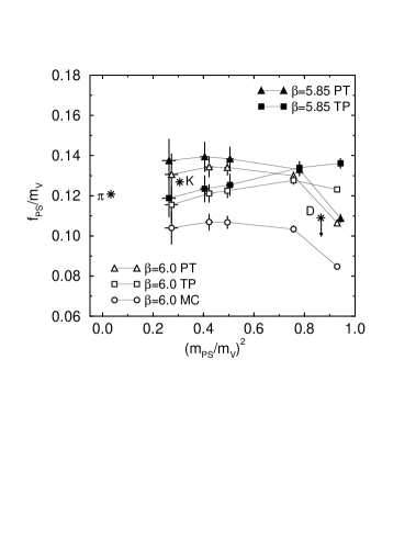
Figure 28: Ratio of the pseudo-scalar meson decay constant to the vector meson mass, for the three choices of renormalization constant discussed in the text. The errors shown are statistical only and are estimated by the jack-knife method. The corresponding experimental values for pseudo-scalar mesons are marked with stars.

We derive $f_{PS}$ from a fit to the $\tilde{\pi}$ propagator. The value of $t_{min}$ is chosen to be the same as that for $\pi$. The pion mass from the $\tilde{\pi}$ propagator is given in table 19. Although the mass obtained is 1 — 2 standard deviations smaller than that from the $\pi$ propagator, they are consistent with each other if we take account of the systematic error. The decay constant at each $K$ is given in table 20. Our data for $f_{PS}^{PT}$ at $\beta=6.0$ and $K=0.155,0.1563$ are consistent with the Ape results [7, 8]. Fig. 28 shows $f_{PS}/m_{V}$ versus $(m_{PS}/m_{V})^{2}$ together with the corresponding experimental values for $\pi$ and $K$ and the upper bound for the $D$ meson. Contrary to the case of the vector meson, $f_{PS}^{MC}$ differs from the experimental value for the $K$ meson by a factor of about 1.2. There is a possibility that the lattice size $10^{3}\times 20$ is not large enough to suppress finite lattice size effects in the Monte Carlo evaluation of $Z_{A}$. We think we have to calculate nonperturbatively $Z_{A}$ both at $\beta=5.85$ and 6.0 on a larger lattice in order to clarify the reason of the discrepancy.

In fig. 25 we show the values of $f_{K}^{TP}/m_{\rho}$ versus $m_{\rho}a$ together with the GF11 result [21]. The values of $f_{K}$ are evaluated at the hopping parameter given by $2/(1/K_{c}+1/K_{s})$. The values of $f_{K}^{TP}/{m_{\rho}}$ are consistent with the GF11 result, albeit with larger errors in our results. Our data at finite lattice spacing are also consistent with experiment.

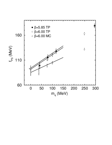
Figure 29: Linear extrapolations of the pseudo-scalar meson decay constant, for the two choices of renormalization constant discussed in the text. The open symbols at zero quark mass are extrapolated values for $\beta=6.0$. The errors shown are statistical only. The experimental value for the pion is marked with a star.

The extrapolation to the chiral limit is problematic. We find that neither of the linear fit to the data at the three largest $K$’s nor the quadratic fit to the data at the four largest $K$’s gives $\chi^{2}/df$ small enough: For $f_{PS}^{TP}$ at $\beta=5.85\ (6.0)$, $\chi^{2}/df=$ 9.1 (6.7) for the linear fit and 9.9 (7.4) for the quadratic fit, respectively. Fits to $f_{PS}^{MC}$ are similar. In Fig. 29 are shown $f_{PS}$ versus the quark mass together with the linear fits. The data at the largest $K$ is much below the fitting lines. Even if we change $t_{min}$, $\chi^{2}/df$ does not reduce much. In Fig. 30 we show $\chi^{2}/df$ together with the result for $f_{PS}^{TP}$ at $\beta=6.0$ versus $t_{min}$. Although $\chi^{2}/df$ is large, the results of the fits are very stable. Therefore we quote the decay constant obtained by the linear extrapolation of the data with $t_{min}=12$ (15) at $\beta=5.85$ (6.0) as the central value of the decay constant. We estimate the systematic errors similarly as in the previous cases with $t_{0}=t_{\chi^{2}}$ — 14 (16) for $\beta=5.85$ (6.0).

These analyses give

		stat.	sys.(fit-range)		sys.(fit-func.)
$\beta=$ 5.85	$f_{\pi}^{TP}=$ 0.0489	$\pm$0.0056	+0.0008	$-$0.0017	+0.0	$-$0.0011
	$f_{\pi}^{TP}=$ 94.1	$\pm$11.8	+1.6	$-$3.3	+0.0	$-$2.2	MeV
$\beta=$6.00	$f_{\pi}^{TP}=$ 0.0394	$\pm$0.0027	+0.0011	$-$0.0	+0.0	$-$0.0013
	$f_{\pi}^{TP}=$ 91.7	$\pm$7.2	+2.7	$-$0.0	+0.0	$-$3.0	MeV
	$f_{\pi}^{MC}=$ 0.0367	$\pm$0.0024	+0.0011	$-$0.0	+0.0	$-$ 0.0014
	$f_{\pi}^{MC}=$ 85.4	$\pm$6.4	+2.5	$-$0.0	+0.0	$-$3.4	MeV

The values of $f_{\pi}$ obtained with the tadpole improved renormalization constants are consistent with the experimental value within the statistical errors (see Fig. 27). That with the MC renormalization constant is also consistent with experiment if we take account of the (small) systematic error. However, we should take these numbers with caution, because $\chi^{2}/df$ for the extrapolation is not small enough as mentioned above. Note that the decay constants in the chiral limit are consistent with the GF11 data [21], although the errors in our results are considerably larger.

7 Conclusions and Discussion

In analyses of numerical simulations toward high precision determination of light hadron masses, one first encounters the problem of fitting range for hadron propagators. We find that effective masses of hadrons in general do not exhibit clear plateaus, although statistics is relatively high (the number of configurations is 100 (200) at $\beta=5.85$ (6.0)). The correlated $\chi^{2}$ fits do not determine unambiguously the time slice beyond which the ground state dominates. We also notice a very intriguing fact that $m_{fit}$ by the correlated fits to a range from $t=t_{0}$ has a strong correlation with $m_{\it eff}$ at $t=t_{0}$. Varying systematically the fitting range, we estimate systematic errors in hadron masses due to statistical fluctuations as well as due to the contamination from excited states, which cannot be properly taken into account by the standard least mean square fit with a fixed fitting range. We find that the systematic errors for the hadron masses with quarks lighter than the strange quark amount to 1 — 2 times the statistical errors.

When the lattice scale is fixed from the $\rho$ meson mass, the masses of the $\Omega^{-}$ baryon and the $\phi$ meson at two $\beta$’s agree with experiment within about one standard deviation. On the other hand, the central value of the nucleon mass at $\beta=6.0$ (5.85) is larger than its experimental value by about 15% (20%) and that of the $\Delta$ mass by about 15% (4%): Even when the systematic errors are included, the baryon masses at $\beta=6.0$ do not agree with experiment. In order to take the continuum limit of the nucleon mass and the $\Delta$ mass, we need data for a wider range of $\beta$ with statistical and systematic errors much reduced. For the masses of excited states of the $\rho$ meson and the nucleon, there exist two-mass fits which do not contradict with experiment, except for the case of the nucleon at $\beta=6.0$. Although this does not necessarily imply that the excited state masses appear consistent with experiment because two-mass fits are very unstable, the existence of such a fit consistent with experiment encourages us to perform more works in this direction.

Determination of meson decay constants is usually accompanied by uncertainties of renormalization constants. One can in principle employ any renormalization constant such as that determined by naive perturbation theory or tadpole improved perturbation theory. We have indeed shown that when we use renormalization constants given by tadpole improved perturbation theory, although the decay constants for the $\phi$, $\rho$, $K$ and $\pi$ mesons are in general off experiment at finite lattice spacing, for example, by 30 — 40% at $m_{\rho}a$ = 0.33 — 0.40 in the case of the $F_{\phi}$, they approach in the continuum limit toward values consistent with the experimental values.

It is, however, desirable to employ a renormalization constant which gives weak $a$ dependence for the decay constants. We have shown that when we use the renormalization constants determined by Monte Carlo simulations, the vector meson decay constants at two $\beta$’s remarkably agree with each other and reproduce the experimental values within the errors for a wide range of the quark mass with the chiral limit included. This implies a strong advantage to apply renormalization constants determined nonperturbatively. For pseudo-scaler mesons, however, we find that although the decay constant $f_{PS}^{MC}$ in the chiral limit agrees with the experimental value of $f_{\pi}$ albeit with large errors, it differs from the experimental value of $f_{K}$ by about 20% at $m_{\rho}a=0.33$. This discrepancy might be due to systematic errors in the numerical calculation of $Z_{A}$. These results imply the importance of more systematic nonperturbative determination of the renormalization constants for various meson decays.

Numerical simulations are performed under the QCDPAX project which is supported by the Grants-in-Aid of Ministry of Education, Science and Culture (Nos. 62060001 and 02402003). Analyses of data are also supported in part by the Grants-in-Aid of Ministry of Education, Science and Culture (Nos. 07NP0401, 07640375 and 07640376).

Note Added

After this work was completed, three groups have reported results of high statistics studies of the hadron spectrum [26, 27, 28] at $\beta=6.0$. Their results are consistent with ours.

$\beta=5.85$			$\beta=6.0$			$m_{\pi}/m_{\rho}$
$K$	#iteration		$K$	#iteration
0.1440	80 $\pm$	3	0.1450	90 $\pm$	3	0.97
0.1540	160 $\pm$	10	0.1520	160 $\pm$	10	0.87
0.1585	420 $\pm$	45	0.1550	380 $\pm$	40	0.70
0.1595	610 $\pm$	75	0.1555	430 $\pm$	45	0.64
0.1605	1850 $\pm$	410	0.1563	1110 $\pm$	170	0.52

Table 1: Hopping parameters and average number of iterations used to solve quark propagators. Approximate values for $m_{\pi}/m_{\rho}$ are also given. Table 8 contains precise values for $m_{\pi}/m_{\rho}$.

$\beta=5.85$
$K$	$\pi$		$\rho$		$N$		$\Delta$
	$t_{\chi^{2}}$	$\chi^{2}/df$	$t_{\chi^{2}}$	$\chi^{2}/df$	$t_{\chi^{2}}$	$\chi^{2}/df$	$t_{\chi^{2}}$	$\chi^{2}/df$
0.1440	12	0.98	12	1.32	11	1.33	11	1.49
0.1540	10	0.90	12	1.01	11	1.61	11	1.61
0.1585	8	0.72	8	2.04	9	1.36	11	1.18
0.1595	8	0.45	8	1.73	9	1.13	11	1.07
0.1605	8	0.46	8	1.20	7	1.56	9	1.30
$\beta=6.0$
$K$	$\pi$		$\rho$		$N$		$\Delta$
	$t_{\chi^{2}}$	$\chi^{2}/df$	$t_{\chi^{2}}$	$\chi^{2}/df$	$t_{\chi^{2}}$	$\chi^{2}/df$	$t_{\chi^{2}}$	$\chi^{2}/df$
0.1450	15	0.55	15	1.02	15	0.36	15	0.57
0.1520	12	1.26	13	0.71	15	0.38	15	0.56
0.1550	10	1.39	11	1.42	12	0.41	12	0.94
0.1555	10	1.35	10	1.32	12	0.64	12	1.22
0.1563	9	1.54	9	0.95	10	1.21	11	1.11

Table 2: $t_{\chi^{2}}$ and $\chi^{2}/df$ at $t_{\chi^{2}}$. See the text for details.

$\beta=5.85$			$\beta=6.0$
$K$	$m_{\pi}$	$\chi^{2}/df$	$K$	$m_{\pi}$	$\chi^{2}/df$
0.1440	1.0293(12)${}^{+2}_{-2}$	13.7/14	0.1450	0.8069(7)${}^{+0}_{-2}$	6.1/11
0.1540	0.6122(11)${}^{+3}_{-6}$	10.9/14	0.1520	0.4772(9)${}^{+9}_{-2}$	11.5/11
0.1585	0.3761(12)${}^{+8}_{-4}$	7.4/14	0.1550	0.2967(15)${}^{+18}_{-5}$	14.1/11
0.1595	0.3088(14)${}^{+6}_{-6}$	5.8/14	0.1555	0.2588(16)${}^{+18}_{-6}$	17.0/11
0.1605	0.2226(21)${}^{+10}_{-7}$	6.0/14	0.1563	0.1847(27)${}^{+20}_{-6}$	20.9/11

Table 3: Pion masses in lattice units. In parentheses are errors estimated by the jack-knife method. Errors given in the form $\mbox{}^{+upper}_{-lower}$ are for the fitting range dependent upper/lower bound.

$\beta=5.85$			$\beta=6.0$
$K$	$m_{\rho}$	$\chi^{2}/df$	$K$	$m_{\rho}$	$\chi^{2}/df$
0.1440	1.0598(15)${}^{+4}_{-1}$	18.5/14	0.1450	0.8370(9)${}^{+2}_{-4}$	11.2/11
0.1540	0.6931(27)${}^{+3}_{-11}$	14.2/14	0.1520	0.5486(15)${}^{+9}_{-11}$	6.6/11
0.1585	0.5294(69)${}^{+115}_{-100}$	28.9/14	0.1550	0.4218(42)${}^{+75}_{-73}$	14.3/11
0.1595	0.4856(96)${}^{+176}_{-123}$	23.2/14	0.1555	0.3982(61)${}^{+135}_{-90}$	12.4/11
0.1605	0.434(20)${}^{+21}_{-24}$	14.6/14	0.1563	0.353(15)${}^{+28}_{-11}$	7.6/11

Table 4: The same as table 3 for the $\rho$ meson.

$K$=0.155
	$\pi$	$\rho$	$N$	$\Delta$
This work $24^{3}\times 54$	0.2967(15)	0.4218(42)	0.6440(85)	0.728(11)
Ape $24^{3}\times 32$ [7]	0.298(2)	0.429(3)	0.647(6)	0.745(15)
Ape $18^{3}\times 64$ [6] smear	0.297(2)	0.430(10)
local	0.297(2)	0.428(8)
LANL $32^{3}\times 64$ [11]	0.297(1)	0.422(3)	0.641(4)	0.706(8)
$K$=0.1563
	$\pi$	$\rho$	$N$	$\Delta$
This work $24^{3}\times 54$	0.1847(27)	0.353(15)	0.536(30)	0.670(53)
Ape $24^{3}\times 32$ [7]	0.184(3)	0.377(8)	0.522(14)	0.636(45)
LANL $32^{3}\times 64$ [11]	0.185(1)	0.363(9)	0.540(12)	0.631(27)

Table 5: Comparison of hadron masses in lattice units at $\beta=6.0$, $K=0.155$ and 0.1563.

$\beta=5.85$			$\beta=6.0$
$K$	$m_{N}$	$\chi^{2}/df$	$K$	$m_{N}$	$\chi^{2}/df$
0.1440	1.6961(50)${}^{+7}_{-18}$	15.8/13	0.1450	1.3225(28)${}^{+15}_{-2}$	3.8/10
0.1540	1.1060(55)${}^{+15}_{-94}$	22.3/13	0.1520	0.8669(49)${}^{+19}_{-3}$	4.2/10
0.1585	0.815(13)${}^{+13}_{-33}$	17.5/13	0.1550	0.6440(85)${}^{+53}_{-12}$	3.8/10
0.1595	0.744(17)${}^{+12}_{-36}$	18.1/13	0.1555	0.6007(109)${}^{+84}_{-7}$	6.2/10
0.1605	0.683(48)${}^{+10}_{-82}$	23.4/13	0.1563	0.536(30)${}^{+58}_{-0}$	15.7/10

Table 6: Nucleon masses in lattice units. In parentheses are errors estimated by the jack-knife method. Errors given in the form $\mbox{}^{+upper}_{-lower}$ are for the fitting range dependent upper/lower bound.

$\beta=5.85$			$\beta=6.0$
$K$	$m_{\Delta}$	$\chi^{2}/df$	$K$	$m_{\Delta}$	$\chi^{2}/df$
0.1440	1.7124(57)${}^{+21}_{-25}$	17.7/13	0.1450	1.3404(29)${}^{+22}_{-1}$	6.2/10
0.1540	1.1629(67)${}^{+37}_{-15}$	20.3/13	0.1520	0.9112(41)${}^{+51}_{-0}$	6.0/10
0.1585	0.9011(153)${}^{+83}_{-57}$	16.5/13	0.1550	0.7278(109)${}^{+188}_{-0}$	12.1/10
0.1595	0.825(21)${}^{+16}_{-37}$	15.1/13	0.1555	0.7001(159)${}^{+336}_{-10}$	15.3/10
0.1605	0.755(53)${}^{+67}_{-78}$	19.4/13	0.1563	0.670(53)${}^{+61}_{-41}$	9.0/10

Table 7: The same as table 6 for the $\Delta$ baryon.

$\beta=5.85$			$\beta=6.0$
$K$	$m_{\pi}/m_{\rho}$	$m_{N}/m_{\rho}$	$K$	$m_{\pi}/m_{\rho}$	$m_{N}/m_{\rho}$
0.1440	0.9712(8)	1.6004(45)	0.1450	0.9641(5)	1.5801(25)
0.1540	0.8833(32)	1.5956(82)	0.1520	0.8699(21)	1.5802(79)
0.1585	0.7104(90)	1.540(29)	0.1550	0.7033(69)	1.527(21)
0.1595	0.636(12)	1.531(42)	0.1555	0.650(10)	1.509(31)
0.1605	0.513(25)	1.57(12)	0.1563	0.523(23)	1.52(10)

Table 8: Mass ratios $m_{\pi}/m_{\rho}$ and $m_{N}/m_{\rho}$. The errors quoted are statistical only and are estimated by the jack-knife method.

		$\rho$ meson		nucleon
	$\beta$	comment	ratio	comment	ratio
This work	5.85	$t_{min}$=5	2.47(16)	$t_{min}=6$	1.64(12)
		$t_{min}$=6	1.87(24)	$t_{min}=7$	1.29(10)
	6.0	$t_{min}$=8	2.21(27)	$t_{min}=7$	1.81(10)
		$t_{min}$=9	1.58(26)
Ape [7]	6.0		2.13(21)		2.13(4)
UKQCD [22]	6.2		2.53(16)		2.01(16)
APE [8]	6.3		1.93(10)		1.93(12)
UKQCD [23]	6.2 Clover		2.23(14)
QCDPAX [5]	6.0	point	1.99(15)	point	1.55(20)
		wall	1.70(26)	wall	1.47(21)
experimental value			1.65

Table 9: Ratios of the excited state mass to the ground state mass. We have taken the quark mass corresponding approximately to the strange quark mass.

	$\beta=5.85$			$\beta=6.0$
	$a_{0}$	$a_{1}$	$\chi^{2}/df$	$a_{0}$	$a_{1}$	$\chi^{2}/df$
$m_{\pi}^{2}$	$-$7.18(4)	1.16(1)	0.56	$-$6.51(6)	1.02(1)	1.06
$m_{\rho}$	$-$6.16(37)	1.06(6)	1.76	$-$6.50(39)	1.07(6)	1.20
$m_{N}$	$-$10.87(51)	1.85(8)	0.37	$-$12.97(79)	2.11(12)	0.05
$m_{\Delta}$	$-$11.37(80)	1.95(13)	0.05	$-$8.4(1.3)	1.42(21)	0.29

Table 10: Fit parameters of the linear fits to the masses at the largest three $K$’s. Errors on $a_{0}$ and $a_{1}$ are those from least mean square fits.

$\beta=5.85$
	value	err-lms	err-jack	jack/lms
$K_{c}$	0.161624	0.000027	0.000033	1.2
$m_{\rho}(K_{c})$	0.400	0.010	0.021	2.1
$m_{N}(K_{c})$	0.589	0.014	0.036	2.6
$m_{\Delta}(K_{c})$	0.664	0.022	0.063	2.9
$\beta=6.0$
	value	err-lms	err-jack	jack/lms
$K_{c}$	0.157096	0.000038	0.000028	0.7
$m_{\rho}(K_{c})$	0.3309	0.0080	0.0114	1.4
$m_{N}(K_{c})$	0.462	0.015	0.024	1.6
$m_{\Delta}(K_{c})$	0.605	0.025	0.033	1.3

Table 11: Values of $K_{c}$ and masses extrapolated to $K_{c}$ determined from the linear fits to the data at the largest three $K$’s. Errors obtained by least mean square fits (err-lms) and those by the jack-knife method (err-jack) together with their ratios (jack/lms) are also given.

$\beta=5.85$				$\beta=6.0$
$t_{0}$	$m_{\rho}$	$a^{-1}$	$\chi^{2}/df$	$t_{0}$	$m_{\rho}$	$a^{-1}$	$\chi^{2}/df$
8	0.4359	1.766	36.90	11	0.3525	2.184	2.51
9	0.4213	1.828	11.17	12	0.3476	2.215	2.54
10	0.4196	1.835	14.80	13	0.3425	2.248	0.77
11	0.4045	1.904	9.30	14	0.3409	2.259	3.94
12	0.3998	1.926	1.76	15	0.3309	2.327	1.20
13	0.3892	1.978	4.39	16	0.3248	2.370	0.17
14	0.4081	1.887	1.36	17	0.3188	2.416	0.58
15	0.3794	2.030	0.43	18	0.3112	2.474	0.03
16	0.3728	2.066	0.11	19	0.3206	2.401	0.00

Table 12: Results of the linear fits to the $\rho$ meson masses versus $t_{0}$. The inverse lattice spacing is defined by $a^{-1}=0.77{\rm GeV}/m_{\rho}(K_{c})$.

$\beta=5.85$				$\beta=6.0$
$t_{0}$	$m_{\rho}$	$a^{-1}$	$\chi^{2}/df$	$t_{0}$	$m_{\rho}$	$a^{-1}$	$\chi^{2}/df$
12	0.3881	1.984	1.22	13	0.3413	2.256	0.79
13	0.3767	2.044	4.02	14	0.3393	2.269	4.33
14	0.3997	1.927	1.20	15	0.3253	2.367	0.91
15	0.3641	2.115	0.21	16	0.3194	2.411	0.07
16	0.3593	2.143	0.30	17	0.3116	2.471	0.41
				18	0.3029	2.542	0.00
				19	0.3146	2.448	0.01

Table 13: Results of the quadratic fits to the $\rho$ meson masses versus $t_{0}$. The inverse lattice spacing is defined by $a^{-1}=0.77{\rm GeV}/m_{\rho}(K_{c})$.

$\beta=5.85$			$\beta=6.0$
$t_{0}$	$m_{N}$	$\chi^{2}/df$	$t_{0}$	$m_{N}$	$\chi^{2}/df$
9	0.6085	3.20	12	0.4828	0.03
10	0.6071	0.37	13	0.4802	0.24
11	0.6039	0.83	14	0.4758	0.79
12	0.5946	2.15	15	0.4759	1.88
13	0.5893	0.37	16	0.4623	0.05
14	0.5680	2.28	17	0.4538	2.00
15	0.5501	1.59	18	0.4553	2.28
16	0.5312	0.49	19	0.4731	0.10
17	0.5630	2.55	20	0.4559	0.10

Table 14: Results of the linear fits to the nucleon masses versus $t_{0}$.

$\beta=5.85$			$\beta=6.0$
$t_{0}$	$m_{\Delta}$	$\chi^{2}/df$	$t_{0}$	$m_{\Delta}$	$\chi^{2}/df$
11	0.6982	0.03	12	0.6055	0.01
12	0.6928	0.01	13	0.6059	4.10
13	0.6640	0.05	14	0.6164	1.78
14	0.6899	4.02	15	0.6279	0.50
15	0.5375	34.96	16	0.6048	0.29
16	0.4757	23.96	17	0.6206	0.12
			18	0.6462	0.17
			19	0.5935	0.34

Table 15: Results of the linear fits to the $\Delta$ masses versus $t_{0}$.

$K$	$Z_{V}$
0.1440	0.5121(9)
0.1540	0.5164(10)
0.1585	0.5126(36)
0.1595	0.5112(48)
0.1605	0.5101(76)
Average	0.5125(30)

Table 16: Renormalization constants $Z_{V}$ for the local lattice current at $\beta=5.85$ obtained in a previous work [2].

$\beta=5.85$				$\beta=6.0$
$K$	$F_{V}^{PT}$	$F_{V}^{TP}$	$F_{V}^{MC}$	$K$	$F_{V}^{PT}$	$F_{V}^{TP}$	$F_{V}^{MC}$
0.1440	0.2214	0.2600(33)${}^{+17}_{-0}$	0.1374	0.1450	0.1753	0.1919(18)${}^{+5}_{-13}$	0.1210
0.1540	0.2211	0.2089(38)${}^{+5}_{-17}$	0.1372	0.1520	0.1673	0.1558(17)${}^{+14}_{-19}$	0.1155
0.1585	0.2094	0.1781(68)${}^{+126}_{-130}$	0.1299	0.1550	0.1544	0.1336(33)${}^{+65}_{-78}$	0.1065
0.1595	0.1996	0.1658(84)${}^{+162}_{-142}$	0.1239	0.1555	0.1493	0.1276(43)${}^{+106}_{-88}$	0.1031
0.1605	0.1885	0.1528(152)${}^{+153}_{-201}$	0.1170	0.1563	0.1382	0.1157(95)${}^{+181}_{-87}$	0.0953

Table 17: $\rho$ meson decay constants in lattice units. In parentheses are errors estimated by the jack-knife method. Errors given in the form $\mbox{}^{+upper}_{-lower}$ are for the fitting range dependent upper/lower bound.

$\beta=5.85$							$\beta=6.0$
	$F_{V}^{TP}$			$F_{V}^{MC}$				$F_{V}^{TP}$			$F_{V}^{MC}$
$t_{0}$	Latt.	Phys.	$\chi^{2}/df$	Latt.	Phys.	$\chi^{2}/df$	$t_{0}$	Latt.	Phys.	$\chi^{2}/df$	Latt.	Phys.	$\chi^{2}/df$
8	0.169	325	53.7	0.133	257	55.7	11	0.127	297	1.9	0.107	250	2.0
9	0.157	303	6.0	0.125	240	7.0	12	0.124	289	1.7	0.105	244	1.9
10	0.156	301	11.1	0.124	239	11.9	13	0.120	280	0.1	0.102	237	0.2
11	0.145	280	5.8	0.115	222	6.3	14	0.120	278	3.4	0.101	235	3.6
12	0.141	271	0.0	0.112	216	0.1	15	0.111	259	0.4	0.094	220	0.4
13	0.130	251	2.3	0.104	201	2.6	16	0.107	248	0.0	0.091	211	0.0
14	0.148	286	0.3	0.118	226	0.3	17	0.101	234	0.1	0.085	199	0.1
15	0.116	224	0.0	0.094	180	0.0	18	0.094	220	0.1	0.080	187	0.1
16	0.105	203	1.1	0.085	164	1.1	19	0.104	243	0.1	0.088	206	0.1

Table 18: Results of the linear fits to the $\rho$ meson decay constants versus $t_{0}$, in lattice units and in physical units (MeV).

$\beta=5.85$						$\beta=6.0$
	$t_{0}=t_{min}=12$		$t_{0}=t_{\chi^{2}}$				$t_{0}=t_{min}=15$		$t_{0}=t_{\chi^{2}}$
$K$	$m_{\tilde{\pi}}$	$\chi^{2}/df$	$t_{\chi^{2}}$	$m_{\tilde{\pi}}$	$\chi^{2}/df$	$K$	$m_{\tilde{\pi}}$	$\chi^{2}/df$	$t_{\chi^{2}}$	$m_{\tilde{\pi}}$	$\chi^{2}/df$
0.1440	1.0299(14)	1.32	8	1.0304	1.68	0.1450	0.8059(9)	0.49	12	0.8068	1.06
0.1540	0.6106(21)	0.96	7	0.6117	1.18	0.1520	0.4747(14)	0.35	7	0.4767	0.91
0.1585	0.3753(34)	0.97	5	0.3774	1.41	0.1550	0.2937(24)	0.88	6	0.2967	0.89
0.1595	0.3070(42)	1.00	4	0.3097	1.45	0.1555	0.2559(30)	0.85	6	0.2593	0.83
0.1605	0.2127(64)	1.02	4	0.2175	1.31	0.1563	0.1804(66)	0.68	5	0.1897	0.75

Table 19: Pion masses determined from $\tilde{\pi}$ propagators.

$\beta=5.85$			$\beta=6.0$
$K$	$f_{PS}^{PT}$	$f_{PS}^{TP}$	$K$	$f_{PS}^{PT}$	$f_{PS}^{TP}$	$f_{PS}^{MC}$
0.1440	0.1152	0.1443(25)${}^{+12}_{-5}$	0.1450	0.0892	0.1030(10)${}^{+12}_{-0}$	0.0710
0.1540	0.0922	0.0929(22)${}^{+10}_{-1}$	0.1520	0.0713	0.0701(11)${}^{+18}_{-0}$	0.0567
0.1585	0.0732	0.0664(26)${}^{+12}_{-14}$	0.1550	0.0566	0.0517(13)${}^{+16}_{-10}$	0.0450
0.1595	0.0677	0.0600(30)${}^{+19}_{-15}$	0.1555	0.0535	0.0482(15)${}^{+15}_{-15}$	0.0426
0.1605	0.0597	0.0515(33)${}^{+32}_{-9}$	0.1563	0.0462	0.0408(26)${}^{+30}_{-23}$	0.0368

Table 20: Pseudo-scalar meson decay constants in lattice units. In parentheses are errors estimated by the jack-knife method. Errors given in the form $\mbox{}^{+upper}_{-lower}$ are for the fitting range dependent upper/lower bound.

Figure 1: Statistical errors in effective masses for the $\rho$ meson at $\beta=6.0$, $K=0.155$ versus the bin size $N_{B}$. The errors are normalized by those for $N_{B}=1$.

Figure 2: Statistical errors in effective masses for the $\rho$ meson at $\beta=6.0$, $K=0.155$ versus the number of configurations $N$. The errors are normalized by those for $N=N_{conf}=200$.

Figure 3: Fitted mass $m_{fit}$ for the pion at $\beta=6.0$, $K=0.155$, obtained from one-mass fit to a range $t$ — $T/2$ and the value of $\chi^{2}/df$ of the fit versus $t$. The error bars for $m_{fit}$ are statistical uncertainties estimated by the least mean square fit. Effective masses $m_{\it eff}$ with errors estimated by the jack-knife method are also given.

Figure 4: The same as Fig. 3 for the $\rho$ meson.

Figure 5: The same as Fig. 3 for the nucleon.

Figure 7: The same as Fig. 6 for the $\rho$ meson: a) $\beta=5.85$, b) $\beta=6.0$.

Figure 8: The same as Fig. 6 for the nucleon: a) $\beta=5.85$, b) $\beta=6.0$.

Figure 9: The same as Fig. 6 for the $\Delta$ baryon: a) $\beta=5.85$, b) $\beta=6.0$.

Figure 10: Nucleon to $\rho$ mass ratio versus pion to $\rho$ mass ratio squared. The errors shown are statistical only. The solid curve is obtained from phenomenological mass formulae[15]. The dotted line is obtained by assuming that $m_{N}/m_{\rho}$ and $(m_{\pi}/m_{\rho})^{2}$ are linear in the quark mass. The experimental value is marked with a star.

Figure 11: Masses of the ground state and the excited state for the $\rho$ meson at $\beta=5.85$, $K=0.1585$ together with the value of $\chi^{2}/df$ of the two-mass fits versus $t_{min}$. The error bars are statistical uncertainties estimated by the least mean square fit. The result of the one-mass fit is reproduced by the solid line, dotted lines and dashed lines for the fitted mass, its statistical error and systematic upper/lower bounds, respectively. Note the difference in the scale of the plots for $m_{0}$ and $m_{1}$.

Figure 12: The same as Fig. 11 for the $\rho$ meson at $\beta=6.0$, $K=0.155$.

Figure 13: The same as Fig. 11 for the nucleon at $\beta=5.85$, $K=0.1585$.

Figure 14: The same as Fig. 11 for the nucleon at $\beta=6.0$, $K=0.155$.

Figure 17: Mass of excited state of the nucleon (denoted by $N^{\prime}$) at $\beta=5.85$ versus $1/K-1/K_{c}$. The experimental values for masses of the nucleon ($N$) and its excited state ($N^{\prime}$) are marked with stars. The data for $m_{N}$, $m_{\rho}$ and $m_{\pi}^{2}$ are taken from the results of one-mass fits. With the scale of the plot, the results for $m_{N}$ from two-mass fits are indistinguishable from the one-mass fit results.

Figure 20: The same as Fig.  19 for $\beta=6.0$.

Figure 23: $a^{-1}$ determined from linear fits to all possible combinations of the $\rho$ masses obtained by varying $t_{0}$ from $t_{\chi^{2}}$ to 18.

Figure 30: Pseudo-scalar meson decay constant at zero quark mass versus $t_{min}$, together with $\chi^{2}/df$. The errors are estimated by the least mean square fit.

References

- [1] Y. Iwasaki and T. Yoshié, Phys. Lett. B216 (1989) 387; Y. Iwasaki, Nucl. Phys. B (Proc. Suppl.) 9 (1989) 254.
- [2] T. Yoshié, Y. Iwasaki and S. Sakai, Nucl. Phys. B (Proc. Suppl.) 17 (1990) 413.
- [3] Ape Collaboration (P. Bacilieri et al.), Phys. Lett. B214 (1988) 115; Ape Collaboration (P. Bacilieri et al.), Nucl. Phys. B317 (1989) 509; Ape Collaboration (S. Cabasino et al.), Nucl. Phys. B (Proc. Suppl.) 17 (1990) 431.
- [4] QCDPAX Collaboration (Y. Iwasaki et al.), Nucl. Phys. B (Proc.Suppl.) 30 (1993) 397.
- [5] QCDPAX Collaboration (Y. Iwasaki et al.), Nucl. Phys. B (Proc.Suppl.) 34 (1994) 354.
- [6] Ape Collaboration (C. R. Allton et al.), Nucl. Phys. B (Proc.Suppl.) 34 (1994) 360.
- [7] Ape Collaboration (S. Cabasino et al.), Phys. Lett. B258 (1991) 195.
- [8] Ape Collaboration (M. Guagnelli et al.), Nucl. Phys. B378 (1992) 616.
- [9] K. M. Bitar et al., Phys. Rev. D46 (1992) 2169.
- [10] F .Butler, H. Chen, J. Sexton, A. Vaccarino and D. Weingarten, Nucl. Phys. B430 (1994) 179.
- [11] T. Bhattacharya and R. Gupta, Nucl. Phys. B (Proc. Suppl.) 42 (1995) 935.
- [12] UKQCD Collaboration (C. R. Allton et al.), Phys. Rev. D49 (1994) 474.
- [13] D. Daniel et al., Phys. Rev. D46 (1992) 3130.
- [14] Y. Iwasaki et al., Computer Physics Communications 49 (1988) 449; T. Shirakawa et al., Proceedings of Supercomputing ’89 495, Reno, USA, Nov. 13-17, 1989; Y. Iwasaki et al., Nucl. Phys. B (Proc. Suppl.) 17 (1990) 259.
- [15] S. Ono, Phys. Rev. D17 (1978) 888.
- [16] G. Martinelli and Y. C. Zhang, Phys. Lett. B123 (1983) 433.
- [17] G. P. Lepage, Nucl. Phys. B (Proc.Suppl.) 26 (1992) 45; A. S. Kronfeld, Nucl. Phys. B (Proc.Suppl.) 30 (1993) 445; P. B. Mackenzie, Nucl. Phys. B (Proc.Suppl.) 30 (1993) 35.
- [18] G. P. Lepage and P. B. Mackenzie, Phys. Rev. D48 (1993) 2250.
- [19] A. X. El-Khadra et al., Phys. Rev. Lett. 69 (1992) 729.
- [20] L. Maiani and G. Martinelli, Phys. Lett. B178 (1986) 265.
- [21] F. Butler, H. Chen, J. Sexton, A. Vaccarino and D. Weingarten, Nucl. Phys. B421 (1994) 217.
- [22] UKQCD Collaboration (C. R. Allton et al.), Phys. Rev. D47 (1993) 5128.
- [23] UKQCD Collaboration (P. Lacock and C. Michael), Phys. Rev. D52 (1995) 5213.
- [24] S. Sharpe, Phys. Rev. D41 (1990) 3233; Phys. Rev. D46 (1992) 3146.
- [25] C. Bernard and M. Golterman, Phys. Rev. D46 (1992) 853.
- [26] JLQCD Collaboration (S. Aoki et al.), Tsukuba preprint UTHEP-323 (hep-lat/9510013), to appear in the Proceedings of Lattice ’95.
- [27] M. Göckeler et al., DESY preprint DESY 95-128 (hep-lat/9508004).
- [28] T. Bhattacharya, R. Gupta, G. Kilcup and S. Sharpe, Los Alamos preprint LA-UR-95-2354 (hep-lat/9512021); T. Bhattacharya and R. Gupta, Los Alamos preprint LA-UR-95-2355 (hep-lat/9510044).