Abstract

We study phases and fractal structures of three-dimensional simplicial quantum gravity by the Monte-Carlo method. After measuring the surface area distribution (SAD) which is the three-dimensional analog of the loop length distribution (LLD) in two-dimensional quantum gravity, we classify the fractal structures into three types: (i) in the hot (strong coupling) phase, strong gravity makes the space-time one crumpled mother universe with small fluctuating branches around it. This is a crumpled phase with a large Hausdorff dimension $d_{\mbox{\tiny H}}\simeq 5$. The topologies of cross-sections are extremely complicated. (ii) at the critical point, we observe that the space-time is a fractal-like manifold which has one mother universe with small and middle size branches around it. The Hausdorff dimension is $d_{\mbox{\tiny H}}\simeq 4$. We observe some scaling behaviors for the cross-sections of the manifold. This manifold resembles the fractal surface observed in two-dimensional quantum gravity. (iii) in the cold (weak coupling) phase, the mother universe disappears completely and the space-time seems to be the branched-polymer with a small Hausdorff dimension $d_{\mbox{\tiny H}}\simeq 2$. Almost all of the cross-sections have the spherical topology $S^{2}$ in the cold phase.

1 Introduction

In recent years remarkable progress has been made to quantize the field theories with general covariance . Especially, in two-dimensional quantum gravity it is very encouraging that some analytical formulations (Liouville field theory[1], matrix models[2], topological field theories[3][4]) and numerical calculations by the dynamical triangulations (DT)[5][6][7] have shown the good agreement. It is found that the universal structure which leads to the continuum limit seems to be its fractal structure[8]. It seems very important to investigate the fractal behavior of the space-time manifold in any dimension. Below, we will briefly review this fractal structure in two dimension as the starting point.

On the other hand, in the three-dimensional quantum gravity which is our primary concern of this paper, as well as in the four-dimensional case, we have no analytical models which predict the scaling or fractal properties near the critical point. By numerical simulations, a few groups have studied the three-dimensional Euclidean quantum gravity based on dynamical triangulations and reported the existence of the first-order phase transition[13][14]. Numerical calculations show that the entropy is exponentially bounded and the thermodynamic limit exists in three-dimensional simplicial gravity[15][16]. The starting point of this model is based on the ansatz that the partition function describing the fluctuations of a continuum geometry can be approximated by a weighted sum over all simplicial manifolds (triangulations) $T$ which is composed of equilateral tetrahedra:

$$Z=\sum_{T}e^{-S_{0}(T)}\thinspace.$$ (1)

In this work the topology of the simplicial lattice is restricted to the three-sphere $S^{3}$. The action is taken to be of the form

$$S_{0}(T)=-\kappa_{0}N_{0}+\kappa_{3}N_{3}\thinspace,$$ (2)

where $N_{i}$ is the number of $i$-simplices in a simplicial lattice $T$, and $\kappa_{0}$, $\kappa_{3}$ are dimensionless gravitational and cosmological constants on the lattice. This action (2) corresponds to a discretized version of the continuum action of three-dimensional Einstein gravity:

$$S_{\mbox{\scriptsize EH}}[g]=-\frac{\displaystyle 1}{\displaystyle G}\int d^{3}x\sqrt{g}R+\lambda\int d^{3}x\sqrt{g}\enspace,$$ (3)

where $G$ is the Newton constant and $\lambda$ is the cosmological constant.

To control the volume fluctuations we add an additional term to the action of the form:

$$\delta S=\gamma\left(N_{3}-V\right)^{2}\enspace,$$ (4)

where $V$ is the target size of the simplicial lattices and $\gamma$ is an appropriate parameter. In ref.[16] it is argued that lattices with $N_{3}\sim V$ are distributed according to the correct Boltzmann weight up to correction terms of order $O(\frac{1}{\sqrt{\gamma}V})$.

In summary, our starting point is the following partition function:

$$Z=\sum_{T}e^{-S(T)}\enspace,$$ (5)

where the total action $S(T)$ on the three-dimensional simplicial lattice is of the form

$$S(T)=-\kappa_{0}N_{0}+\kappa_{3}N_{3}+\gamma\left(N_{3}-V\right)^{2}\enspace.$$ (6)

Now, we would like to explain the method to detect the fractal structure, taking two-dimensional quantum gravity as an example in some detail. Let us consider a triangulated surface $\mit\Sigma$ which is composed of equilateral triangles. One of the points to understand the continuum limit of the DT in two dimension is its fractal structure[8], characterized by the loop length distribution (LLD) defined as follows:

1. Let us consider a $\phi^{3}$-graph $\tilde{\mit\Sigma}$ dual to the triangulated surface $\mit\Sigma$.

2. Pick up a single point $P$ in $\tilde{\mit\Sigma}$ (a triangle in $\mit\Sigma$).

3. Find all the points which has a geodesic distance (= minimum number of steps of two points in the dual graph) $D$ from $P$.

4. The set of links (also links in $\mit\Sigma$) connecting two points of distance $D-1$ and $D$ consists of some closed loops in $\mit\Sigma$.

5. We define the loop length distribution (LLD) function by counting the number of these closed loops which have a geodesic distance $D$ and a loop length $L$, and write $g(L,D)$.

As shown in ref.[8], the function $g(L,D)$ is universal and explicitly calculated as

$$g(L,D)\times D^{2}=\frac{\displaystyle 3}{\displaystyle 7\sqrt{\pi}}(x^{-5/2}+\frac{\displaystyle 1}{\displaystyle 2}x^{-3/2}+\frac{\displaystyle 14}{\displaystyle 3}x^{1/2})e^{-x}$$ (7)

with $x=L/D^{2}$ as a scaling parameter. Numerically, this fractal behavior was established by N.Tsuda and T.Yukawa[10][11].

In the next section, we will explain our data and the interpretations of the measurements will be described, mainly on the three-dimensional analog of the fractal structure described above.

2 Numerical simulations

To discuss the phase structure of simplicial gravity, the integrated scalar curvature per volume has conventionally been used. The lattice analog is:

$$\frac{\displaystyle\int d^{3}x\sqrt{g}R}{\displaystyle\int d^{3}x\sqrt{g}}\quad\longrightarrow\quad\sum_{l}\frac{\displaystyle\left(c-n(l)\right)}{\displaystyle N_{3}}=c\frac{\displaystyle N_{0}}{\displaystyle N_{3}}-(6-c)\enspace,$$ (8)

where $c=2\pi/\arccos(1/3)=5.104\dots$ is the number of tetrahedra around a link which gives the zero scalar curvature for flat space. Here $n(l)$ denotes the number of tetrahedra sharing the link $l$, called the coordination number. A conventional indicator of phase transitions is the specific heat, which in this case corresponds to the fluctuation in the number of vertices $N_{0}$:

$$\chi_{N_{0}}=\frac{\displaystyle 1}{\displaystyle V}(\langle N_{0}^{2}\rangle-\langle N_{0}\rangle^{2})\enspace,$$ (9)

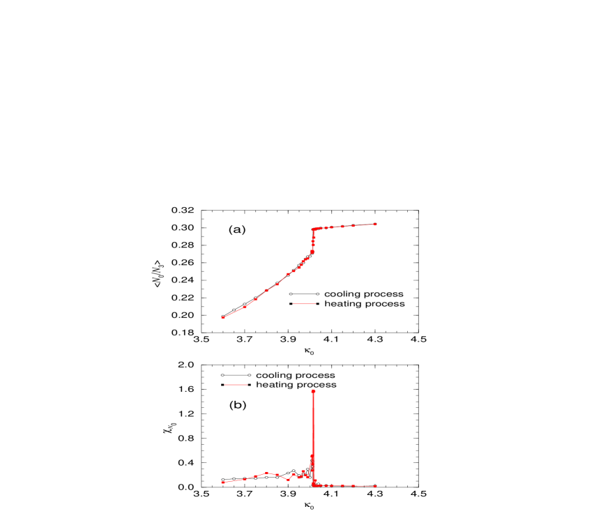
Figure 1: Cooling and heating processes with lattice size $V$ = 10000. (a)Scalar curvature per volume .vs. $\kappa_{0}$ for each process. No hysteresis is observed. (b)Node susceptibility .vs. $\kappa_{0}$

where averages are taken over ensembles of configurations with a fixed volume $N_{3}=V$. In fig.1, we show the expectation value $<N_{0}/N_{3}>$ and $\chi_{N_{0}}$ as a function of the gravitational coupling constant $\kappa_{0}$. We cannot observe the hysteresis curve, in contrast to the calculation in ref.[13]. We observe a phase transition near $\kappa_{0}=4.0$, but with this data above, we cannot determine the order of the transition unless performing the finite-size scaling analysis.

Here we should make a remark about the thermalization in our study which will explain the difference from the paper[13]. For the error estimate we used the jackknife method[20]. We examined the magnitude of error as a function of the bin size and adopted the bin size where the jackknife error had leveled off. This bin size corresponds to about 500 sweeps where one sweep is defined as the total number of accepted moves divided by the number of tetrahedra $N_{3}$. Comparing to the typical interval of about 100 sweeps in two dimension, the relaxation time of the Markov chain in three dimension is much longer. We need to perform computer runs with the long interval larger than 500 sweeps to accumulate the statistically uncorrelated data. We have taken the interval 600 sweeps to calculate our data. The reason why the hysteresis has disappeared in fig.1 is that we have thermalized our data enough to avoid the autocorrelation. In ref.[13], $10^{3}$ sweeps were taken to get each point in the hysteresis, but we have taken $600\times 120=7.2\times 10^{4}$ sweeps to get each point in the fig.1. No hysteresis is often observed in a finite system, though there exists a first-order transition in the system[17]. We cannot determine the order of the transition without performing the finite-size scaling analysis[18].

In general, if a statistical system has a second-order phase transition, some scaling invariant properties, or, fractal structures are expected to appear at the critical point. In the case of two-dimensional gravity, the LLD characterizes the fractal property of the surface[8] as described in the last section. By the analogy to two-dimensional case, we introduce the surface area distribution (SAD) in three-dimensional case:

1. Let us consider a connected $\phi^{4}$-graph $\tilde{T}$ dual to a three-dimensional simplicial lattice $T$ with a spherical topology $S^{3}$.

2. Pick up a single point $P$ in $\tilde{T}$ (a tetrahedron in $T$).

3. Find all the points which has a geodesic distance (= minimum number of steps of two points in the dual graph) $D$ from $P$.

4. The set of links (triangles in $T$) connecting two points of distance $D-1$ and $D$ consist of some closed surfaces in $T$.

5. We define the distribution function of these closed surfaces which have a distance $D$ and area $A$ as surface area distribution (SAD), and denote by $f(A,D)$.

Theoretically, there exist no analytical models which predict the scaling behavior of this SAD function $f(A,D)$. We have measured the SAD functions in the case of the lattice size $V=10000$. At each distance $D$, we compute the number of branches (baby universes) $N_{\mbox{\scriptsize b}}(D)$, the volume within the distance $V(D)$ , and moreover the large area ($\equiv$ the cross-section of the mother universe) $A_{\mbox{\scriptsize large}}(D)$. In general, we expect these observables to scale as,

$$N_{\mbox{\scriptsize b}}(D) \sim D^{d_{\mbox{\tiny b}}}\thinspace,$$

$$V(D)\hskip 0.28436pt \sim D^{d_{\mbox{\tiny H}}}\thinspace,$$ (10)

$$A_{\mbox{\scriptsize large}}(D) \sim D^{d_{\mbox{\tiny M}}}\thinspace.$$

If the manifold (space-time) has a mother body (huge universe) which dominates the fractal structure, we expect $d_{\mbox{\scriptsize H}}=d_{\mbox{\scriptsize M}}+1$.

In fig.2, we show the data in the strong coupling limit $\kappa_{0}=0$. There exists a huge mother universe. The behavior of $N_{\mbox{\scriptsize b}}(D)$ in fig.2(a) is similar to that of the crumpled surface in two-dimensional quantum gravity[11]. From the linear region $D\simeq 8$ in fig.2(b), we can read $V(D)\sim D^{5}$, or the Hausdorff dimension $d_{\mbox{\scriptsize H}}\simeq 5$. In fig.2(c), we show the SAD with $x=A/D^{4}$ as a scaling variable, because this variable gives the most proper fitting for the distribution of the large area ($\equiv$ cross-section of the mother universe). Fig.2(d) also shows that the large area should scale as $A_{\mbox{\scriptsize large}}(D)\sim D^{4}$, consistent with the naive expectation $d_{\mbox{\scriptsize H}}=d_{\mbox{\scriptsize M}}+1$. In fig.2(c), we can observe no contributions from the universes of middle size. These facts give us the picture that the space-time manifold has one extremely crumpled huge mother universe which is not expanding widely and many small baby universes of low density are fluctuating around it. The SAD function for the mother universe which dominates the fractal structure of the manifold seems to indicate a scaling behavior with a scaling variable $x=A/D^{4}$.

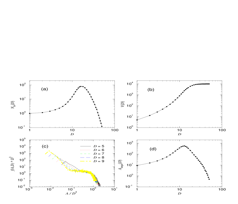
Figure 3: The data at the critical point ($\kappa_{0}=4.0$). (a)Number of branches at each distance $D$. (b)Volume within the geodesic distance $D$. (c)The SAD is shown with the scaling parameter $x=A/D^{3}$. (d) The expectation value of the large area.

Next, the data near the critical point $\kappa_{0}=4.0$ are shown in fig.3. The behavior of $N_{\mbox{\scriptsize b}}(D)$ in fig.3(a) is very similar to that of the fractal surface in two-dimensional quantum gravity[11]. This is one of the reasons why we call the manifold at the critical point fractal-like. We can read $d_{\mbox{\scriptsize b}}\simeq 3$ from fig.3(a). From the linear region in fig.3(b), we can read the Hausdorff dimension $d_{\mbox{\scriptsize H}}\simeq 4$. Our data show the existence of the mother universe, which extends more widely than that of the hot phase. Fig.3(d) shows that the large area ($\equiv$ cross-section of the mother universe) scales as $A_{\mbox{\scriptsize large}}\sim D^{3}$, giving the same Hausdorff dimension $d_{\mbox{\scriptsize H}}\simeq 4$. So we choose $x=A/D^{3}$ as the scaling variable, but the small and middle areas ($\equiv$ rest parts after subtracting the contribution of the mother) do not scale as well by this variable in fig.3(c). Then, we divide the SAD function into two parts, the contribution of the large area $f_{\mbox{\scriptsize large}}(A,\thinspace D)$ and rest of areas (hereafter we abbreviate small and middle areas to small areas) $f_{\mbox{\scriptsize small}}(A,\thinspace D)\thinspace$:

$$f(A,\thinspace D)=f_{\mbox{\scriptsize large}}(A,\thinspace D)+f_{\mbox{\scriptsize small}}(A,\thinspace D)\thinspace.$$ (11)

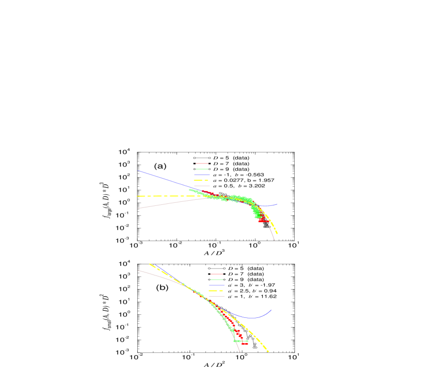
Figure 4: The divided SAD function at the critical point ($\kappa_{0}=4.0$). (a)The SAD for the large part measured and some fittings. (b)The SAD for the small part measured and some fittings.

The divided data in fig.4(b) tells us that $x^{\prime}=A/D^{2}$ is a good scaling variable for the dominant part of $f_{\mbox{\scriptsize small}}(A,\thinspace D)$.

Let us discuss the fractal(-like) structure at the critical point in some detail. In fig.4(a), we can assume the large area distribution function as,

$$f_{\mbox{\scriptsize large}}(A,\thinspace D)=const.\times\frac{\displaystyle 1}{\displaystyle D^{3}}\thinspace x^{a}e^{-bx}\thinspace.$$ (12)

Here $a$ and $b$ are some constants. The fittings in the fig.4(a) show that we can safely assume $a>-1$, so the integration of $f_{\mbox{\scriptsize large}}(A,\thinspace D)$ given in eq.(12) is convergent. In other words, the following quantities are finite:

$$\langle A^{n}\rangle_{\mbox{\scriptsize large}}=\thinspace\lim_{\epsilon\to 0}\int^{\infty}_{\epsilon}dA\thinspace A^{n}f_{\mbox{\scriptsize large}}(A,\thinspace D)\hskip 28.45274pt(n\geq 0)\thinspace.$$ (13)

Here $\epsilon$ is the cutoff for the area on the simplicial lattice. It is easy to show that

$$\langle A^{0}\rangle_{\mbox{\scriptsize large}} \propto \mit\Gamma(a+\mbox{1})\times D^{\mbox{\scriptsize 0}}\thinspace,$$

$$\langle A^{1}\rangle_{\mbox{\scriptsize large}} \propto \mit\Gamma(a+\mbox{2})\times D^{\mbox{\scriptsize 3}}\thinspace.$$ (14)

From eq.(14), the large area part (mother universe) is independent of the cutoff $\epsilon$, so this part seems to be the universal quantity.

On the other hand, from fig.4(b) the small area distribution function is parametrized as,

$$f_{\mbox{\scriptsize small}}(A,\thinspace D)=const.\times\frac{\displaystyle 1}{\displaystyle D^{2}}\thinspace x^{\prime-a^{\prime}}e^{-b^{\prime}x^{\prime}}\thinspace.$$ (15)

Here $a^{\prime}$ and $b^{\prime}$ are positive constants. From the gradient of the dominant line in the fig.4(b), we can read the value of the exponent $a^{\prime}=2/5$. The good fitting function (after rescaling $b^{\prime}x^{\prime}\to x^{\prime}$) is the following form:

$$f_{\mbox{\scriptsize small}}(A,\thinspace D)=const.\times\frac{\displaystyle 1}{\displaystyle D^{2}}\thinspace x^{\prime-5/2}e^{-x^{\prime}}\thinspace.$$ (16)

Then, we can calculate the quantity:

$$\langle A^{0}\rangle_{\mbox{\scriptsize small}} = \int^{\infty}_{\epsilon}dA\thinspace f_{\mbox{\scriptsize small}}(A,\thinspace D)$$ (17)

$$\propto const.\times D^{3}\epsilon^{-3/2}+const.\times D\epsilon^{-1/2}+const.\times D^{0}\thinspace,$$

$$\langle A^{1}\rangle_{\mbox{\scriptsize small}} = \int^{\infty}_{\epsilon}dA\thinspace A\thinspace f_{\mbox{\scriptsize small}}(A,\thinspace D)$$ (18)

$$\propto const.\times D^{3}\epsilon^{-1/2}+const.\times D^{2}\thinspace.$$

Moreover, the average area of the small part behaves as

$$\langle A^{1}\rangle_{\mbox{\scriptsize small}}/\langle A^{0}\rangle_{\mbox{\scriptsize small}}\thinspace\sim\thinspace\epsilon\thinspace.$$ (19)

This relation (19) is quite similar to the two-dimensional fractal surface where the small loop has a constant length with the size of the cutoff length[8]. The small baby universe is not a universal quantity but also a local quantum fluctuation. If we identify

$$\langle A^{0}\rangle_{\mbox{\scriptsize small}}=N_{\mbox{\scriptsize b}}(D)\sim D^{d_{\mbox{\tiny b}}}\thinspace,$$ (20)

then we can decide $d_{\mbox{\tiny b}}=3$ by comparing eq.(17) and eq.(20). This value of $d_{\mbox{\tiny b}}=3$ accounts very well for the behavior of $N_{\mbox{\scriptsize b}}(D)$ in fig.3(a). Moreover, eq.(18) and eq.(14) give the same Hausdorff dimension $d_{\mbox{\scriptsize H}}=4$, accounting for the behavior of $V(D)$ in fig.3(b).

Here we mention the observation by Agishtein and Migdal[9]. It was found in ref.[9] that the Hausdorff dimension $d_{\mbox{\scriptsize H}}$ grows logarithmically

$$d_{\mbox{\scriptsize H}}\sim c_{1}+c_{2}\log D\hskip 56.9055pt(c_{1},c_{2}\enspace\mbox{are constants})\thinspace.$$ (21)

They argued that the logarithmic growth of Hausdorff dimension might be a universal law of Nature. But, in our interpretation, this behavior (21) expresses the non-universal (cutoff-dependent) property which originates in the small part (see eq.(18)).

Now we can explain the notion of the fractal-like manifold. At the critical point, the mother, middle and small universes contribute to the SAD function as well as to the LLD function of the fractal surface in two-dimensional quantum gravity[8]. But the distinct point is the observation that we have two kinds of scaling variables, $x=A/D^{3}$ for the mother and $x^{\prime}=A/D^{2}$ for the baby universes in three-dimensional quantum gravity. This is why we call such a manifold not fractal but fractal-like. It is a remarkable property of three-dimensional fractal-like manifold that both the large and small areas give the same Hausdorff dimension $d_{\mbox{\scriptsize H}}\simeq 4$, though the large area gives $d_{\mbox{\scriptsize H}}=3$ but the dominant small areas give $d_{\mbox{\scriptsize H}}=4$ in two-dimensional fractal manifold[8].

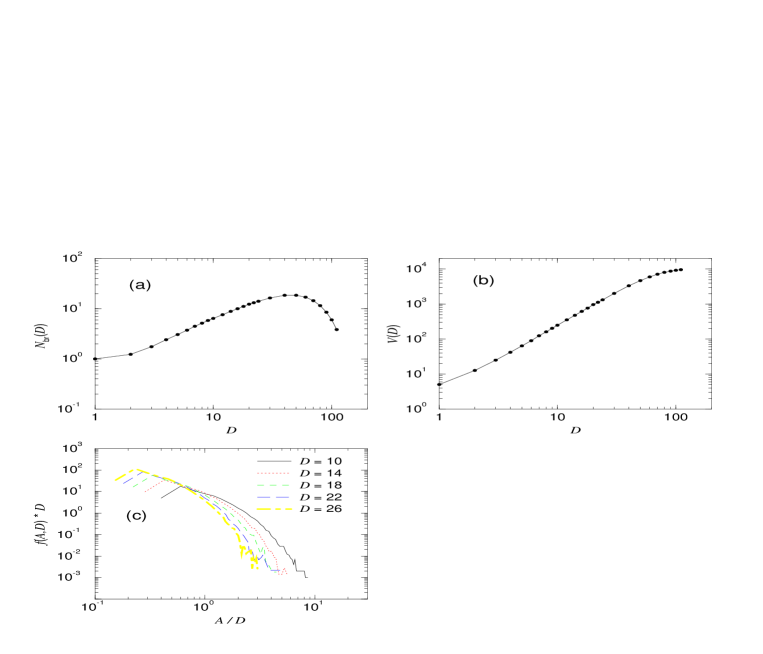
Figure 5: The data in the cold phase ($\kappa_{0}=5.0$). (a)Number of branches at each distance $D$. (b)Volume within the geodesic distance $D$. (c)The SAD is shown with the scaling parameter $x=A/D$.

Finally, we show the data in the weak coupling phase (cold phase) $\kappa_{0}=5.0$ in fig.5. In this phase, the space-time manifold consists of widely expanding branches and has no mother universe. Fig.5(a) shows $N_{\mbox{\scriptsize b}}(D)\sim D$. The behavior of $N_{\mbox{\scriptsize b}}(D)$ is quite different from the other cases, but similar to that of the branched-polymer in two-dimensional gravity[11]. From fig.5(b), we can easily read that $V(D)\sim D^{2}$, or $d_{\mbox{\scriptsize H}}\simeq 2$. Because the mother body does not exist in this phase, we should choose a scaling variable $x=A/D$ for the dominant small fluctuations in fig.5(c).

3 Summary and discussion

There exist two phases, hot and cold phase, in three-dimensional simplicial quantum gravity, as previously known[12][14]. They argued the first-order transition between these two phases because of the existence of a large hysteresis[13]. In our study we observed a rapid transition near $\kappa_{0}=4.0$ but no hysteresis, so we cannot determine the order of the transition without the finite-size scaling analysis.

By measuring the SAD functions using the Monte-Carlo technique, we could characterize the phases of three-dimensional simplicial gravity into three types:

1. The hot phase (strong coupling phase).
       This phase is a typical crumpled phase. Strong gravity makes the space-time a crumpled manifold with small fluctuations around it. The fact that the area of the cross-section of the mother universe scales as $A_{\mbox{\scriptsize large}}(D)\sim D^{4}$ determines the Hausdorff dimension to be $d_{\mbox{\scriptsize H}}\simeq 5$. The topology of the cross-sections for the mother universe is highly complicated, though those of baby universes are almost spherical topologies. Because the contribution of the baby universes to the SAD function is quite different from that of the mother in contrast to the LLD in two dimension, we do not know how one associates a fractal structure with this case.

2. The critical point.
       At this point, the space-time is a fractal-like manifold. By the term fractal-like, we means that this manifold seems to have two different scaling variables, $x=A/D^{3}$ for the mother universe, and $x^{\prime}=A/D^{2}$ for the baby universes. Both the long and short distance regions give the same Hausdorff dimension $d_{\mbox{\scriptsize H}}\simeq 4$. The fractal behavior of the long distance part seems to be universal or cutoff-independent. The topologies of the cross-sections are less complicated than those in the hot phase.

3. The cold phase (weak coupling phase).
       In this phase, the mother universe, which exists in the hot phase and at the critical point, disappears completely. Weak gravity cannot make any large body in the space-time. The fractal structure is determined by the dominant small fluctuations with a scaling parameter $x=A/D$. Almost all of the cross-sections have the spherical topology $S^{2}$. The space-time is a branched-polymer with a small Hausdorff dimension $d_{\mbox{\scriptsize H}}\simeq 2$. We could not find any universal (cutoff-independent) property in this phase.

We should discuss the properties at the critical point in more detail. Because three-dimensional Einstein-Hilbert action (3) includes a dimensionfull coupling constant $G$, this theory is perturbatively unrenormalizable as well as four-dimensional Einstein gravity. In other words, we cannot expect the scale invariance over all order of scales in such a theory. But our data shows that two different types of scaling regions seem to exist near the critical point, short distance region (small baby universe) and long distance region (mother universe). Short distance region has its own scaling with a scaling variable $x^{\prime}=A/D^{2}$. But this region seems to be cutoff-dependent, so we cannot expect the universal structure in this region. On the other hand, long distance region also has its own scaling with a scaling variable $x=A/D^{3}$. As the scaling of this region seems to be cutoff-independent, this fractal-like structure may be a universal one which leads to the continuum limit as well as the fractal structure does in two-dimensional lattice gravity. This point is very important. To confirm our conjecture, we added the irrelevant discretized $R^{2}$-term to the Einstein-Hilbert action (6) on the simplicial lattice. Though the SAD function of the small part changed its form, that of the mother part did not change its form when the coupling to $R^{2}$-term is small[19]. But these facts do not establish the universality of the fractal-like SAD function, so we need further studies based on the method in constructive field theory and interesting results are expected.

Acknowledgements
    We would like to thank the members of KEK theory group for discussions. We are especially grateful to H.Kawai and N.Ishibashi for useful discussions and critical comments.

Figure 2: The data in the hot phase (strong coupling limit $\kappa_{0}=0$). (a)Number of branches at each distance $D$. (b)Volume within the geodesic distance $D$. (c)The SAD is shown with a scaling parameter $x=A/D^{4}$. (d) The expectation value of the large area.

References

-
[1]
J.Distler and H.Kawai, Nucl.Phys. B321 (1989) 509;
V.G.Knizhnik, A.M.Polyakov and A.B.Zamolodchikov, Mod.Phys.Lett. A3 (1988) 819 -
[2]
D.J.Gross and A.A.Migdal, Nucl.Phys. B340 (1990) 333;
M.R.Dougras and S.H.Shenker, Nucl.Phys. B335 (1990) 635;
F.David,Nucl.Phys. B257[FS14] (1985) 45. -
[3]
J.Distler, Nucl.Phys. B342 (1990) 523;
E.Verlinde and H.Verlinde,Nucl.Phys. B348 (1990) 457. - [4] For a review of topological field theory, see D.Birmingham, M.Blau, M.Rakowski and G.Thompson, Topological field theory, Phys.Rep. 209 No.4 & 5 (1991) 129.
- [5] J.Ambjørn, B.Durhuus and J.Fröhlich, Nucl.Phys. B257[FS14] (1985) 433; Nucl.Phys. B275[FS17] (1986) 161.
- [6] D.V.Boulatov, V.A.Kazakov, I.K.Kostov and A.A.Migdal, Nucl.Phys. B275[FS17] (1986) 641.
- [7] J.Jurkiewick, A.Krzywicki, B.Perterson and Søderberg, Phys.Lett. B213 (1988) 511.
- [8] H.Kawai, N.Kawamoto, T.Mogami and Y.Watabiki, Phys.Lett. B306 (1993) 19.
- [9] M.E.Agishtein and A.A.Migdal, Mod.Phys.Lett. A6, N0.20 (1991) 1863.
- [10] N.Tsuda and T.Yukawa, Phys.Lett. B305 (1993) 223.
- [11] N.Tsuda and T.Yukawa, 2D quantum gravity, three states of surfaces, KEK-CP-039.
- [12] D.V.Boulatov and A.Krzywicki, Mod.Phys.Lett. A6 No.32 (1991) 3005.
- [13] J.Ambjørn, D.V.Boulatov, A.Krzywicki and S.Varsted, Phys.Lett. B276 (1992) 432.
- [14] J.Ambjørn and S.Varsted, Nucl.Phys. B373 (1992) 557.
- [15] J.Ambjørn and S.Varsted, Phys.Lett. B266 (1991) 285.
- [16] S.Catterall, J.Kogut and R.Renken, Entropy and the approach to the thermodynamic limit in three-dimensional simplicial gravity, CERN-TH.7404/94, ILL-(TH)-94-20.
- [17] M.Fukugita, H.Mino, M.Okawa and A.Ukawa, J.Phys.A:Math.Gen. 23 (1990) L561.
- [18] Murty S.S.Challa and D.P.Landau and K.Binder, Phys.Rev. B34 No.3 (1986) 1841.
- [19] As for the -gravity in three dimension, we will report our results elsewhere.
-
[20]
B.Efron, SIAM Rev. 21 (1979) 460;
R.G.Miller, Biometrika 61 (1974) 1.