INLO-PUB-20/95

Abstract: We study the properties of the electroweak sphaleron on a finite lattice. The cooling algorithm for saddle points is used to obtain the static classical solutions of the SU(2)-Higgs field theory. Results are presented for $M_{H}=\infty,\,M_{W},\,{\scriptstyle{{3\over 4}}}M_{W}$. After performing finite size scaling we find good agreement with the results obtained from variational approaches. Of relevance for numerical determinations of the transition rate is that the lattice artefacts are surprisingly small for $M_{W}\approx M_{H}$.

1 Introduction

In this paper we will study the sphaleron solutions for the SU(2)-Higgs field theory, using the lattice approximation and an algorithm to find saddle-point solutions. The sphaleron is a solution of the static equations of motion, i.e. a stationary point of the energy functional, which has precisely one unstable direction. This direction corresponds to the tunnelling path associated to the (approximate) instanton. Due to the spherical symmetry, variational analysis using a radial ansatz has provided accurate results quite some time ago [1, 2]. However, due to the recent interest of studying the sphaleron transition rates on a lattice [3], the question arises how big the lattice artefacts are for the particular sizes of lattices that are employed in the numerical analysis. The lattice destroys the rotational invariance and a variational analysis does no longer seem very practical. Furthermore, in the absence of rotational symmetry in the continuum, the method discussed can be used with the same ease.

We have reported earlier [4] on the sphaleron solutions where the length of the Higgs field is frozen. In the unitary gauge this means that we only need to consider gauge degrees of freedom. We recall that above $M_{H}=12M_{W}$ the sphaleron undergoes a series of bifurcations [5], acquiring at each bifurcation an additional negative mode, while new solutions, so-called deformed sphalerons split off. For infinite $M_{H}$, where the model is identical to the gauged non-linear sigma model, there is an infinite number of solutions ranging in energy from $5.41M_{W}/\alpha_{W}$ to the energy of the lowest deformed sphaleron $5.07M_{W}/\alpha_{W}$, which has only one negative mode (the number of unstable modes increases with increasing energy). These solutions are related to the electroweak skyrmions [6].

Here we will include the scalar field in the analysis to allow study of the electroweak sphalerons (at $\theta_{W}=0$) for a more interesting range of parameters. We will report results for $M_{H}=M_{W}$ and $M_{H}={\scriptstyle{{3\over 4}}}M_{W}$, the latter value corresponding to $M_{H}\approx 60$GeV, the present experimental bound for the Higgs mass [7]. Since for finite values of the Higgs self-coupling the scalar field is allowed to vanish at the center, these solutions are smoother (have smaller lattice artefacts) than for the electroweak skyrmions. We first present the new algorithm to find the extremum of the energy functional, based on minimizing the square of the equations of motion. A careful analysis of the finite size scaling is performed, to allow for a reliable extrapolation to the infinite volume limit. The results agree accurately with those obtained from the variational analysis. For $M_{H}=M_{W}$ the lattice artefacts are to a good degree described by the formula $E=E_{0}-0.3(aM_{W})^{2}-0.3(aM_{W})^{4}$, whereas the volume corrections are described by $3.641+18.1(M_{W}L)^{-1}e^{-M_{W}L}$ (the infinite volume variational result [5] is 3.6417) all in units of $M_{W}/\alpha_{W}$, where $\alpha_{W}=g^{2}/4\pi$ is the electroweak fine-structure constant.

2 The model

The dynamical variables for the SU(2)-Higgs model on the lattice are the gauge group variables $V_{\mu}(x)$, defined on the link that runs from $x$ to $x+\hat{\mu}$, and the Higgs field in the fundamental representation of SU(2) (a complex two-component spinor) defined on the site $x$. This Higgs field can be represented by its length $\rho(x)$ (in the continuum this neutral Higgs field will be denoted by $\phi(x)$) and a SU(2) matrix $\sigma(x)$, which is associated to the gauge degree of freedom and can be reabsorbed into the links via the change of variables [8]

$$U_{\mu}(x)=\sigma(x)V_{\mu}(x)\sigma(x+\mu).$$ (1)

This gives the Higgs model in the unitary gauge. The lattice action is ($U_{\mu}(x)=\raisebox{-5.69046pt}{ \begin{picture}(1.2,1.2)(-0.6,-0.6)\put(0.5,0.0){\line(-1,0){1.0}} \put(0.0,0.0){\vector(1,0){0.1}} \put(-0.5,0.0){\circle*{0.2}} \put(-0.35,-0.25){\makebox(0.0,0.0)[tr]{\footnotesize$x$}} \put(0.4,-0.3){\makebox(0.0,0.0)[r]{\footnotesize$\mu$}} \end{picture}}$)

$$S\!=\!\frac{a^{n}}{g^{2}a^{4}}\!\sum_{x}\!\left\{\sum_{\mu,\nu}\!\!\mbox{\,Tr\,}\!\left(1\!\!-\!\raisebox{-5.69046pt}{ \begin{picture}(1.2,1.2)(-0.6,-0.6) \put(-0.5,-0.5){\line(1,0){1.0}} \put(0.5,-0.5){\line(0,1){1.0}} \put(0.5,0.5){\line(-1,0){1.0}} \put(-0.5,0.5){\line(0,-1){1.0}} \put(0.0,-0.5){\vector(1,0){0.0}} \put(0.5,0.0){\vector(0,1){0.0}} \put(0.0,0.5){\vector(-1,0){0.0}} \put(-0.5,0.0){\vector(0,-1){0.0}}\put(-0.5,-0.5){\circle*{0.2}} \put(-0.6,-0.6){\makebox(0.0,0.0)[tr]{\footnotesize$x$}} \put(-0.55,0.4){\makebox(0.0,0.0)[r]{\footnotesize$\nu$}} \put(0.4,-0.6){\makebox(0.0,0.0)[t]{\footnotesize$\mu$}} \end{picture}}\right)\!-\!\kappa\!\!\sum_{\mu}\!\rho(x)\rho(x\!+\!\hat{\mu})\mbox{\,Tr\,}\!\left(U_{\mu}(x)\right)\!+\!\rho^{2}(x)\!+\!\lambda(\rho^{2}(x)\!-\!1)^{2}\!-\!C_{0}\right\}.\\$$ (2)

For $n=4$ ($n=3$) the continuum action (energy) functional is recovered by rescaling the fields and coupling constants. Introducing a lattice spacing $a$, to convert to dimensionful parameters, one first scales the fields to get the correct normalizations for the kinetic terms.

$$U_{\mu}(x)=\exp(aA_{\mu}(x)),\quad A_{\mu}(x)=-igA_{\mu}^{a}(x)\frac{\tau_{a}}{2},\quad\rho^{2}(x)=\frac{a^{2}g^{2}}{2\kappa}\phi^{2}(x),$$ (3)

where $\tau_{a}$ are the Pauli matrices. The continuum parameters $M_{W}$, $M_{H}$ and $\bar{\lambda}$ are given by

$$\bar{\lambda}=\frac{g^{2}\lambda}{4\kappa^{2}},\quad(aM_{W})^{2}=\frac{\kappa v^{2}}{2},\quad(aM_{H})^{2}=\frac{4\lambda v^{2}}{\kappa},$$ (4)

with $v$ the lattice vacuum expectation value

$$v^{2}=\frac{8\kappa+2\lambda-1}{2\lambda}.$$ (5)

Introducing the parameters

$$\bar{\kappa}\equiv 2M_{W}^{2}a^{2},\quad r\equiv M_{H}/M_{W},$$ (6)

one can eliminate $\lambda$ and $\kappa$ in favour of these more physical parameters

$$\lambda=\frac{r^{2}\kappa^{2}}{8},\quad\kappa=\frac{-(32-\bar{\kappa}r^{2})+\sqrt{(32-\bar{\kappa}r^{2})^{2}+16r^{2}}}{2r^{2}}.$$ (7)

Note that for $r\rightarrow\infty$, $v\rightarrow 1$ and $\kappa\rightarrow\bar{\kappa}$.

In this paper we are interested in the energy functional, with $U_{0}(x)=I$, and all fields time independent. Note that restricting the sums over the indices to three dimensions leaves an extra term $-2\kappa\rho^{2}(x)$ from the time component of the hopping term. We have chosen our conventions such that the gauge coupling constant can be factored out, allowing us to express the energies in units of $M_{W}/\alpha_{W}$

$${\cal E} = \frac{M_{W}}{2\pi\alpha_{W}\sqrt{2\bar{\kappa}}}\!\sum_{x}\!\Bigl{\{}\sum_{\mu,\nu}\!\!\mbox{\,Tr\,}\!\left(1\!\!-\!\raisebox{-5.69046pt}{ \begin{picture}(1.2,1.2)(-0.6,-0.6) \put(-0.5,-0.5){\line(1,0){1.0}} \put(0.5,-0.5){\line(0,1){1.0}} \put(0.5,0.5){\line(-1,0){1.0}} \put(-0.5,0.5){\line(0,-1){1.0}} \put(0.0,-0.5){\vector(1,0){0.0}} \put(0.5,0.0){\vector(0,1){0.0}} \put(0.0,0.5){\vector(-1,0){0.0}} \put(-0.5,0.0){\vector(0,-1){0.0}}\put(-0.5,-0.5){\circle*{0.2}} \put(-0.6,-0.6){\makebox(0.0,0.0)[tr]{\footnotesize$x$}} \put(-0.55,0.4){\makebox(0.0,0.0)[r]{\footnotesize$\nu$}} \put(0.4,-0.6){\makebox(0.0,0.0)[t]{\footnotesize$\mu$}} \end{picture}}\right)\!-\!\kappa\!\!\sum_{\mu}\!\rho(x)\rho(x\!+\!\hat{\mu})\mbox{\,Tr\,}\!\left(U_{\mu}(x)\right)\!+\!(1\!-\!2\kappa)\rho^{2}(x)$$ (8)

$$\hskip 199.16928pt+\lambda(\rho^{2}(x)\!-\!1)^{2}\!\!-\!C_{0}\Bigr{\}}.$$

From now on all indices are assumed to run over the values 1-3. The constant $C_{0}$ normalizes the vacuum ($U_{\mu}(x)\equiv I$ and $\rho(x)\equiv v$) energy to zero,

$$C_{0}=(1\!-\!8\kappa)v^{2}\!+\!\lambda(v^{2}\!-\!1)^{2}=\lambda\!-\!{\scriptstyle{{1\over 2}}}(aM_{H})^{2}(aM_{W})^{2}.$$ (9)

For ease of reference we quote the continuum expression for the energy functional in the unitary gauge using our conventions ($F_{\mu\nu}\!=\!\partial_{\mu}A_{\nu}\!-\!\partial_{\nu}A_{\mu}\!+\![A_{\mu},A_{\nu}]\equiv-igF_{\mu\nu}^{a}\tau_{a}/2$)

$${\cal E}=\frac{1}{2g^{2}}\!\int d^{3}x|\mbox{\,Tr\,}(F_{\mu\nu})^{2}|\!+\!\int d^{3}x\left[{\scriptstyle{{1\over 2}}}(\partial_{\mu}\phi)^{2}\!-\!{\scriptstyle{{1\over 4}}}\mbox{\,Tr\,}(A^{2}_{\mu})\phi^{2}\!+\!\bar{\lambda}\left(\phi^{2}\!-\!M_{H}^{2}/8\bar{\lambda}\right)^{2}\right],$$ (10)

3 Cooling

Cooling algorithms [9] are designed to find a solution for the equations of motion associated to a local minimum of the energy functional. It is relatively easy to write down the lattice equations of motion. In particular it should be noted that the energy functional depends linearly on the links. One finds

$$\partial_{U_{\mu}(x)}{\cal E}\propto U_{\mu}(x)\tilde{U}^{\dagger}_{\mu}(x)\!-\!\tilde{U}_{\mu}(x)U^{\dagger}_{\mu}(x)=0,\quad\partial_{\rho(x)}{\cal E}\propto\rho(x)\Bigl{\{}1\!-\!2\kappa\!+\!2\lambda(\rho^{2}(x)\!-\!1)\Bigr{\}}\!-\!\tilde{\rho}(x)=0,$$ (11)

where

$$\tilde{U}_{\mu}(x)={\scriptstyle{{1\over 2}}}\kappa\rho(x)\rho(x\!+\!\hat{\mu})+\tilde{U}_{\mu}(x;0),\quad\tilde{U}_{\mu}(x;0)=\sum_{\nu\neq\mu}\left(\raisebox{-5.69046pt}{ \begin{picture}(1.2,1.2)(-0.6,-0.6)\put(0.5,-0.5){\line(0,1){1.0}} \put(0.5,0.5){\line(-1,0){1.0}} \put(-0.5,0.5){\line(0,-1){1.0}} \put(0.5,0.0){\vector(0,-1){0.0}} \put(0.0,0.5){\vector(1,0){0.0}} \put(-0.5,0.0){\vector(0,1){0.0}} \put(-0.5,-0.5){\circle*{0.2}} \put(-0.45,-0.65){\makebox(0.0,0.0)[tr]{\footnotesize$x$}} \put(-0.55,0.0){\makebox(0.0,0.0)[r]{\footnotesize$\nu$}} \put(0.1,0.7){\makebox(0.0,0.0)[b]{\footnotesize$\mu$}} \end{picture}}+\raisebox{-5.69046pt}{ \begin{picture}(1.2,1.2)(-0.6,-0.6)\put(0.5,-0.5){\line(0,1){1.0}} \put(0.5,-0.5){\line(-1,0){1.0}} \put(-0.5,0.5){\line(0,-1){1.0}} \put(0.5,0.0){\vector(0,1){0.0}} \put(0.0,-0.5){\vector(1,0){0.0}} \put(-0.5,0.0){\vector(0,-1){0.0}} \put(-0.5,0.5){\circle*{0.2}} \put(-0.6,0.85){\makebox(0.0,0.0)[tr]{\footnotesize$x$}} \put(-0.55,0.0){\makebox(0.0,0.0)[r]{\footnotesize$\nu$}} \put(0.0,-0.6){\makebox(0.0,0.0)[t]{\footnotesize$\mu$}} \end{picture}}\right),$$ (12)

$$\tilde{\rho}(x)={\scriptstyle{{1\over 2}}}\kappa\sum_{\mu}\rho(x\!+\!\hat{\mu})\mbox{\,Tr\,}(U_{\mu}(x))+\rho(x\!-\!\hat{\mu})\mbox{\,Tr\,}(U_{\mu}(x\!-\!\hat{\mu})).$$ (13)

The equations of motion for the links are solved by

$$U_{\mu}(x)=\pm\tilde{U}_{\mu}(x)/\|\tilde{U}_{\mu}(x)\|.$$ (14)

The positive sign is to be taken in order for the solution to have a smooth continuum limit. The solution for the scalar field $\rho(x)$ is given by the root of a cubic polynomial. If $1\!-\!2\kappa\!-\!2\lambda\!\geq\!0$, equivalent to the condition $(aM_{H})^{2}\!\leq\!12$, there is only one real root, $\rho(x)=\rho_{s}(\tilde{\rho}(x))$, where

$$\rho_{s}(\tilde{\rho})\equiv\left[\frac{\tilde{\rho}}{4\lambda}\!+\!\sqrt{\left(\frac{1\!-\!2\kappa\!-\!2\lambda}{6\lambda}\right)^{3}\!+\!\frac{\tilde{\rho}^{2}}{16\lambda^{2}}}\ \right]^{\scriptstyle{{1\over 3}}}\!+\left[\frac{\tilde{\rho}}{4\lambda}\!-\!\sqrt{\left(\frac{1\!-\!2\kappa\!-\!2\lambda}{6\lambda}\right)^{3}\!+\!\frac{\tilde{\rho}^{2}}{16\lambda^{2}}}\ \right]^{\scriptstyle{{1\over 3}}}.$$ (15)

Cooling is performed by iterating these equations, i.e. replacing the link and the scalar field by the right-hand side of these equations, sweeping in a particular order through the lattice. With only nearest-neighbour interactions, checkerboard-type updates are most efficient and allow for vectorization of the algorithm. We use this cooling to first bring a random configuration down to one that is smooth. But since the solutions we are interested in have an unstable direction, we should switch to an algorithm that does not make the solution decay along the unstable direction (to the vacuum). This is achieved by taking the square of the equations of motion as the minimizing functional [10], and devising an efficient algorithm for minimization [11, 4]. There are of course more sophisticated algorithms to avoid decay along an unstable direction, but they tend to require information on the Hessian of the energy functional, which is expensive for large lattices.

4 Saddle-point cooling

We define $\hat{S}$ by summing the squares of the equations of motion, $(\partial_{U_{\mu}(x)}{\cal E})^{2}$ and $(\partial_{\rho(x)}{\cal E})^{2}$,

$$\hat{S}=\frac{1}{g^{2}a^{3}}\sum_{x,\mu}\Bigl{\{}\mbox{\,Tr\,}\!\left(\!\tilde{U}_{\mu}(x)\tilde{U}_{\mu}^{\dagger}(x)\!-\![U_{\mu}(x)\tilde{U}_{\mu}^{\dagger}(x)]^{2}\!\right)\!+\!f\left(\rho(x)\left[1\!-\!2\kappa\!+\!2\lambda(\rho^{2}(x)\!-\!1)\right]\!-\!\tilde{\rho}(x)\right)^{2}\Bigr{\}},$$ (16)

where $f$ is an arbitrary positive constant. One can show that in the continuum limit ($D_{\mu}F_{\mu\nu}\equiv\partial_{\mu}F_{\mu\nu}\!+\![A_{\mu},F_{\mu\nu}]$)

$$\hat{S}=\frac{2}{g^{2}}\!\int d^{3}x|\mbox{\,Tr\,}(D_{\mu}F_{\mu\nu}\!-\!{\scriptstyle{{1\over 4}}}A_{\nu}\phi^{2})^{2}|\!+\!\frac{f\kappa}{2}\!\int d^{3}x\left[\partial_{\mu}^{2}\phi\!-\!4\bar{\lambda}\phi^{3}\!+\!{\scriptstyle{{1\over 2}}}\mbox{\,Tr\,}(A^{2}_{\mu})\phi\!+{\scriptstyle{{1\over 2}}}\!M_{H}^{2}\phi\right]^{2},$$ (17)

which has the dimension of $M_{W}^{3}$. Consequently, we will quote values of $\hat{S}$ in units of $M_{W}^{3}/\alpha_{W}$. For $r$ finite, $\kappa$ has a non-zero limit when $a\rightarrow 0$ (e.g. $\kappa(a=0,r=1)=0.1245$), we therefore took $f=1$. Saddle-point cooling introduced in ref. [11] is designed to minimize $\hat{S}$ down to its minimal value of zero. The value of $\hat{S}$ is a direct measure for how close the cooled configuration is to an exact lattice solution.

Finding an algorithm to minimize $\hat{S}$ is more complicated due to the quadratic dependence on the link variables. It is not possible to analytically find the minimum of $\hat{S}$ as a function of a single given link, keeping all others (and $\rho(x)$) fixed. If $f=0$, where the scalar degree of freedom is absent, the following algorithm [11, 4] always lowers $\hat{S}$

$$U^{\prime}_{\mu}(x)={M(U_{\mu}(x))-W_{\mu}(x)\over{\|M(U_{\mu}(x))-W_{\mu}(x)\|}}.$$ (18)

We use the same algorithm here and add the prescription for updating the scalar field. The definitions of $W_{\mu}(x)$ and $M(U_{\mu}(x))$ (specifying the parts of $\hat{S}$ respectively linear and quadratic in $U_{\mu}(x)$) will be split according to

$$M(U_{\mu}(x)) = M^{(0)}(U_{\mu}(x))\!+\!M^{(1)}(U_{\mu}(x))\!+\!fM^{(2)}(U_{\mu}(x)),$$

$$W_{\mu}(x) = W^{(0)}_{\mu}(x)\!+\!W^{(1)}_{\mu}(x)\!+\!fW^{(2)}_{\mu}(x),$$ (19)

where the index 0 stands for the pure gauge part ($\kappa=0$, see ref. [11]), the index 1 for the $\kappa$ dependent term arising through the modified link equations of motion [4], cmp. eqs. (11,12), and the index 2 stands for the part that comes from the scalar equations of motion. Using the notation of $V_{\mu}^{\alpha}(x)$ for the $2(n\!-\!1)$ staples in eq. (12), we have

$$M^{(0)}(U_{\mu}(x))+M^{(1)}(U_{\mu}(x)) \equiv 2\mbox{\,Tr\,}\left(U_{\mu}(x)\tilde{U}_{\mu}^{\dagger}(x)\right)\tilde{U}_{\mu}(x)+6\sum_{\alpha}\mbox{\,Tr\,}\left(U_{\mu}(x)V_{\mu}^{\alpha}(x)^{\dagger}\right)V_{\mu}^{\alpha}(x),$$

$$M^{(2)}(U_{\mu}(x)) \equiv -\frac{\kappa^{2}}{2}\left\{\rho^{2}(x)+\rho^{2}(x\!+\!\hat{\mu})\right\}\mbox{\,Tr\,}\left(U_{\mu}(x)\right),$$ (20)

and

$$W^{(0)}_{\mu}(x) = 2\sum_{\stackrel{{\scriptstyle a\neq-b}}{{a,b\neq\pm\mu}}}\raisebox{-14.22636pt}{ \begin{picture}(1.2,1.2)(-0.6,-0.6)\put(0.25,-0.5){\line(0,1){1.0}} \put(0.25,0.5){\line(-1,0){0.5}} \put(-0.25,0.5){\line(0,-1){1.0}} \put(-0.25,0.0){\line(1,0){0.1}} \put(-0.1,0.0){\line(1,0){0.1}} \put(0.05,0.0){\line(1,0){0.1}} \put(0.2,0.0){\line(1,0){0.05}} \put(-0.25,-0.5){\circle*{0.1}} \put(-0.25,0.5){\circle*{0.1}} \put(0.25,-0.5){\circle*{0.1}} \put(0.25,0.5){\circle*{0.1}} \put(-0.25,0.0){\circle*{0.1}} \put(0.25,0.0){\circle*{0.1}} \put(-0.25,-0.15){\vector(0,1){0.0}} \put(-0.25,0.35){\vector(0,1){0.0}} \put(0.1,0.5){\vector(1,0){0.0}} \put(0.25,0.15){\vector(0,-1){0.0}} \put(0.25,-0.35){\vector(0,-1){0.0}} \put(0.0,-0.55){\makebox(0.0,0.0)[tr]{\footnotesize$x$}} \put(-0.34,-0.3){\makebox(0.0,0.0)[r]{\footnotesize$a$}} \put(-0.43,0.3){\makebox(0.0,0.0)[t]{\footnotesize$b$}} \put(0.0,0.8){\makebox(0.0,0.0)[t]{\footnotesize$\mu$}} \end{picture}}-\raisebox{-14.22636pt}{ \begin{picture}(1.2,1.2)(-0.6,-0.6)\put(-0.29,-0.5){\line(0,1){0.54}} \put(-0.29,0.04){\line(1,0){0.54}} \put(0.25,0.04){\line(0,1){0.46}} \put(0.25,0.5){\line(-1,0){0.46}} \put(-0.21,0.5){\line(0,-1){0.4}} \put(-0.21,-0.04){\line(1,0){0.46}} \put(0.25,-0.04){\line(0,-1){0.46}} \put(-0.25,-0.5){\circle*{0.1}} \put(-0.21,0.5){\circle*{0.1}} \put(0.25,0.5){\circle*{0.1}} \put(-0.29,-0.5){\circle*{0.1}} \put(0.25,-0.5){\circle*{0.1}} \put(-0.29,-0.15){\vector(0,1){0.0}} \put(-0.21,0.25){\vector(0,-1){0.0}} \put(-0.1,0.5){\vector(-1,0){0.0}} \put(0.2,-0.04){\vector(1,0){0.0}} \put(0.1,0.04){\vector(1,0){0.0}} \put(0.25,0.35){\vector(0,1){0.0}} \put(0.25,-0.35){\vector(0,-1){0.0}} \put(-0.3,-0.6){\makebox(0.0,0.0)[tr]{\footnotesize$x$}} \put(-0.38,-0.3){\makebox(0.0,0.0)[r]{\footnotesize$a$}} \put(0.4,0.45){\makebox(0.0,0.0)[t]{\footnotesize$b$}} \put(0.0,0.3){\makebox(0.0,0.0)[t]{\footnotesize$\mu$}} \end{picture}}+2\sum_{\stackrel{{\scriptstyle a\neq-\mu}}{{b\neq\pm\mu,\pm a}}}\raisebox{-14.22636pt}{ \begin{picture}(1.2,1.2)(-0.6,-0.6)\put(-0.5,-0.25){\line(0,1){0.5}} \put(-0.5,0.25){\line(1,0){1.0}} \put(0.5,0.25){\line(0,-1){0.5}} \put(0.5,-0.25){\line(-1,0){0.5}} \put(0.0,-0.25){\line(0,1){0.1}} \put(0.0,-0.1){\line(0,1){0.1}} \put(0.0,0.05){\line(0,1){0.1}} \put(0.0,0.2){\line(0,1){0.1}} \put(-0.5,-0.25){\circle*{0.1}} \put(0.0,-0.25){\circle*{0.1}} \put(0.5,-0.25){\circle*{0.1}} \put(-0.5,0.25){\circle*{0.1}} \put(0.0,0.25){\circle*{0.1}} \put(-0.5,0.25){\circle*{0.1}} \put(-0.5,0.1){\vector(0,1){0.0}} \put(-0.15,0.25){\vector(1,0){0.0}} \put(0.35,0.25){\vector(1,0){0.0}} \put(0.5,-0.1){\vector(0,-1){0.0}} \put(0.2,-0.25){\vector(-1,0){0.0}} \put(0.0,-0.3){\makebox(0.0,0.0)[tr]{\footnotesize$x$}} \put(0.35,0.42){\makebox(0.0,0.0)[r]{\footnotesize$a$}} \put(-0.65,0.15){\makebox(0.0,0.0)[t]{\footnotesize$b$}} \put(-0.25,0.5){\makebox(0.0,0.0)[t]{\footnotesize$\mu$}} \end{picture}}-\raisebox{-14.22636pt}{ \begin{picture}(1.2,1.2)(-0.6,-0.6)\put(-0.5,-0.25){\line(0,1){0.54}} \put(-0.5,0.29){\line(1,0){0.54}} \put(0.5,0.21){\line(-1,0){0.4}} \put(0.5,0.21){\line(0,-1){0.46}} \put(0.5,-0.25){\line(-1,0){0.46}} \put(0.04,0.29){\line(0,-1){0.54}} \put(-0.04,0.21){\line(0,-1){0.46}} \put(-0.5,-0.25){\circle*{0.1}} \put(0.5,-0.25){\circle*{0.1}} \put(-0.5,0.29){\circle*{0.1}} \put(0.5,0.21){\circle*{0.1}} \put(-0.5,0.1){\vector(0,1){0.0}} \put(-0.15,0.29){\vector(1,0){0.0}} \put(0.2,0.21){\vector(-1,0){0.0}} \put(0.04,-0.05){\vector(0,-1){0.0}} \put(-0.04,-0.15){\vector(0,-1){0.0}} \put(0.5,0.1){\vector(0,1){0.0}} \put(0.35,-0.25){\vector(1,0){0.0}} \put(-0.55,-0.3){\makebox(0.0,0.0)[tr]{\footnotesize$x$}} \put(0.35,-0.42){\makebox(0.0,0.0)[r]{\footnotesize$a$}} \put(-0.65,0.15){\makebox(0.0,0.0)[t]{\footnotesize$b$}} \put(-0.25,0.54){\makebox(0.0,0.0)[t]{\footnotesize$\mu$}} \end{picture}}+\raisebox{-14.22636pt}{ \begin{picture}(1.2,1.2)(-0.6,-0.6)\put(-0.5,-0.25){\line(0,1){0.5}} \put(-0.5,0.25){\line(1,0){1.0}} \put(0.5,0.25){\line(0,-1){0.5}} \put(0.0,-0.25){\line(-1,0){0.5}} \put(0.0,-0.25){\line(0,1){0.1}} \put(0.0,-0.1){\line(0,1){0.1}} \put(0.0,0.05){\line(0,1){0.1}} \put(0.0,0.2){\line(0,1){0.1}} \put(-0.5,-0.25){\circle*{0.1}} \put(0.0,-0.25){\circle*{0.1}} \put(0.5,-0.25){\circle*{0.1}} \put(-0.5,0.25){\circle*{0.1}} \put(0.0,0.25){\circle*{0.1}} \put(-0.5,0.25){\circle*{0.1}} \put(-0.5,0.1){\vector(0,1){0.0}} \put(0.35,0.25){\vector(1,0){0.0}} \put(-0.15,0.25){\vector(1,0){0.0}} \put(0.5,-0.05){\vector(0,-1){0.0}} \put(-0.35,-0.25){\vector(-1,0){0.0}} \put(0.1,-0.35){\makebox(0.0,0.0)[tr]{\footnotesize$x$}} \put(0.37,0.42){\makebox(0.0,0.0)[r]{\footnotesize$\mu$}} \put(-0.65,0.15){\makebox(0.0,0.0)[t]{\footnotesize$b$}} \put(-0.25,0.5){\makebox(0.0,0.0)[t]{\footnotesize$a$}} \end{picture}}-\raisebox{-14.22636pt}{ \begin{picture}(1.2,1.2)(-0.6,-0.6)\put(0.5,-0.25){\line(0,1){0.54}} \put(0.5,0.29){\line(-1,0){0.54}} \put(-0.5,0.21){\line(1,0){0.4}} \put(-0.5,0.21){\line(0,-1){0.46}} \put(-0.5,-0.25){\line(1,0){0.46}} \put(-0.04,0.29){\line(0,-1){0.54}} \put(0.04,0.21){\line(0,-1){0.46}} \put(0.5,-0.25){\circle*{0.1}} \put(-0.5,-0.25){\circle*{0.1}} \put(0.5,0.29){\circle*{0.1}} \put(-0.5,0.21){\circle*{0.1}} \put(0.5,-0.1){\vector(0,-1){0.0}} \put(0.35,0.29){\vector(1,0){0.0}} \put(-0.35,0.21){\vector(-1,0){0.0}} \put(-0.04,0.05){\vector(0,1){0.0}} \put(0.04,0.2){\vector(0,1){0.0}} \put(-0.5,-0.1){\vector(0,-1){0.0}} \put(-0.15,-0.25){\vector(1,0){0.0}} \put(0.15,-0.35){\makebox(0.0,0.0)[tr]{\footnotesize$x$}} \put(-0.2,-0.42){\makebox(0.0,0.0)[r]{\footnotesize$a$}} \put(-0.15,0.15){\makebox(0.0,0.0)[t]{\footnotesize$b$}} \put(0.25,0.54){\makebox(0.0,0.0)[t]{\footnotesize$\mu$}} \end{picture}}$$

$$W^{(1)}_{\mu}(x) = \kappa\!\!\sum_{a\neq\pm\mu}\!\!\rho(x\!+\!\hat{\mu}\!\!+\!\hat{a})\Bigl{\{}\rho(x\!+\!\hat{a})(\raisebox{-5.69046pt}{ \begin{picture}(1.2,1.2)(-0.6,-0.6)\put(0.5,-0.5){\line(0,1){1.0}} \put(-0.5,0.5){\line(1,0){0.2}} \put(-0.2,0.5){\line(1,0){0.2}} \put(0.1,0.5){\line(1,0){0.2}} \put(0.4,0.5){\line(1,0){0.1}} \put(-0.5,0.5){\line(0,-1){1.0}} \put(0.5,0.0){\vector(0,-1){0.0}} \put(-0.5,0.0){\vector(0,1){0.0}} \put(-0.5,-0.5){\circle*{0.2}} \put(-0.6,-0.6){\makebox(0.0,0.0)[tr]{\footnotesize$x$}} \put(0.0,0.0){\makebox(0.0,0.0)[r]{\footnotesize$a$}} \put(0.1,0.8){\makebox(0.0,0.0)[b]{\footnotesize$\mu$}} \end{picture}}-\!\!\raisebox{-5.69046pt}{ \begin{picture}(1.2,1.2)(-0.6,-0.6)\put(0.5,-0.5){\line(0,1){1.1}} \put(0.5,0.6){\line(-1,0){0.85}} \put(-0.5,0.45){\line(1,0){0.85}} \put(-0.5,0.45){\line(0,-1){0.95}} \put(0.5,0.0){\vector(0,-1){0.0}} \put(0.4,0.62){\vector(1,0){0.0}} \put(0.1,0.45){\vector(1,0){0.0}} \put(-0.5,0.0){\vector(0,1){0.0}} \put(-0.5,-0.5){\circle*{0.2}} \put(-0.6,-0.6){\makebox(0.0,0.0)[tr]{\footnotesize$x$}} \put(0.0,0.0){\makebox(0.0,0.0)[r]{\footnotesize$a$}} \put(0.1,0.85){\makebox(0.0,0.0)[b]{\footnotesize$\mu$}} \end{picture}}\ )+\rho(x\!+\!\hat{\mu})\raisebox{-5.69046pt}{ \begin{picture}(1.2,1.2)(-0.6,-0.6)\put(0.5,-0.5){\line(0,1){1.0}} \put(0.5,0.5){\line(-1,0){1.0}} \put(-0.5,0.5){\line(0,-1){1.0}} \put(0.5,0.0){\vector(0,-1){0.0}} \put(0.0,0.5){\vector(1,0){0.0}} \put(-0.5,0.0){\vector(0,1){0.0}} \put(-0.5,-0.5){\circle*{0.2}} \put(-0.6,-0.6){\makebox(0.0,0.0)[tr]{\footnotesize$x$}} \put(0.0,0.0){\makebox(0.0,0.0)[r]{\footnotesize$a$}} \put(0.1,0.7){\makebox(0.0,0.0)[b]{\footnotesize$\mu$}} \end{picture}}\ (\raisebox{-5.69046pt}{ \begin{picture}(0.6,0.6)(-0.6,-0.6)\put(-0.5,0.5){\line(0,-1){1.0}} \put(-0.5,0.0){\vector(0,1){0.0}} \put(0.2,-0.6){\makebox(0.0,0.0)[tr]{\footnotesize$x\!+\!\hat{\mu}$}} \end{picture}}\!-\!\raisebox{-5.69046pt}{ \begin{picture}(0.6,0.6)(-0.6,-0.6)\put(-0.5,0.5){\line(0,-1){1.0}} \put(-0.5,0.0){\vector(0,-1){0.2}} \put(0.2,-0.6){\makebox(0.0,0.0)[tr]{\footnotesize$x\!+\!\hat{\mu}$}} \end{picture}})\Bigr{\}}\!+\!\rho(x)\rho(x\!+\!\hat{a})\times$$

$$\hskip 22.76219pt(\raisebox{-5.69046pt}{ \begin{picture}(0.4,0.6)(-0.6,-0.6)\put(-0.5,0.5){\line(0,-1){1.0}} \put(-0.5,0.0){\vector(0,-1){0.2}} \put(-0.5,-0.5){\circle*{0.2}} \put(-0.6,-0.6){\makebox(0.0,0.0)[tr]{\footnotesize$x$}} \put(-0.55,0.3){\makebox(0.0,0.0)[r]{\footnotesize$a$}} \end{picture}}-\raisebox{-5.69046pt}{ \begin{picture}(0.4,0.6)(-0.6,-0.6)\put(-0.5,0.5){\line(0,-1){1.0}} \put(-0.5,0.0){\vector(0,1){0.0}} \put(-0.5,-0.5){\circle*{0.2}} \put(-0.6,-0.6){\makebox(0.0,0.0)[tr]{\footnotesize$x$}} \put(-0.55,0.3){\makebox(0.0,0.0)[r]{\footnotesize$a$}} \end{picture}})\raisebox{-5.69046pt}{ \begin{picture}(1.2,1.2)(-0.6,-0.6)\put(0.5,-0.5){\line(0,1){1.0}} \put(0.5,0.5){\line(-1,0){1.0}} \put(-0.5,0.5){\line(0,-1){1.0}} \put(0.5,0.0){\vector(0,-1){0.0}} \put(0.0,0.5){\vector(1,0){0.0}} \put(-0.5,0.0){\vector(0,1){0.0}} \put(-0.5,-0.5){\circle*{0.2}} \put(-0.6,-0.6){\makebox(0.0,0.0)[tr]{\footnotesize$x$}} \put(0.0,0.0){\makebox(0.0,0.0)[r]{\footnotesize$a$}} \put(0.1,0.7){\makebox(0.0,0.0)[b]{\footnotesize$\mu$}} \end{picture}}\ =\kappa\!\!\sum_{a\neq\pm\mu}\!\!\rho(x\!+\!\hat{\mu}\!+\!\hat{a})U_{a}(x)\Bigl{\{}\rho(x\!+\!\hat{a})(I\!\!-\!U^{2}_{\mu}(x\!+\!\hat{a}))U^{\dagger}_{a}(x\!+\!\hat{\mu})+$$

$$\hskip 14.22636pt\rho(x\!+\!\hat{\mu})U_{\mu}(x\!+\!\hat{a})(I\!\!-\!U^{\dagger}_{a}(x\!+\!\hat{\mu})^{2})\Bigr{\}}\!+\!\rho(x)\rho(x\!+\!\hat{a})(I\!\!-\!U_{a}^{2}(x))U_{\mu}(x\!+\!\hat{a})U_{a}^{\dagger}(x\!+\!\hat{\mu})$$

$$W^{(2)}_{\mu}(x) = \kappa\rho(x)\Bigl{\{}\frac{\kappa}{2}\sum_{a\neq-\mu}\rho(x\!+\!\hat{\mu}\!+\!\hat{a})\mbox{\,Tr\,}(U_{a}(x\!+\!\hat{\mu}))\!-\!\rho(x\!+\!\hat{\mu})(1\!-\!2\kappa\!+\!2\lambda(\rho^{2}(x\!+\!\hat{\mu})\!-\!1))\Bigr{\}}+$$ (21)

$$\hskip 14.22636pt\kappa\rho(x+\hat{\mu})\Bigl{\{}\frac{\kappa}{2}\sum_{a\neq\mu}\rho(x\!+\!\hat{a})\mbox{\,Tr\,}(U_{a}(x))-\rho(x)(1\!-\!2\kappa\!+\!2\lambda(\rho^{2}(x)\!-\!1))\Bigr{\}},$$

with the unit vectors $\hat{a},\hat{b}\in\{\pm\hat{1},\cdots,\pm\hat{n}\}$, and the convention $U_{-a}(x)\equiv U_{a}^{\dagger}(x-\hat{a})$. We only give the explicit form for $W_{\mu}^{(1)}(x)$ and $W_{\mu}^{(2)}(x)$, referring for $W^{(0)}_{\mu}(x)$ to eq. (19) of ref. [11]. To implement this algorithm it is useful to point out that $W^{(0)}_{\mu}(x)$ can be obtained by a sum over all links in each staple of $\tilde{U}_{\mu}(x;0)$ (see eq. (12)), with each link $U_{\ell}$ replaced by the sum over $2U_{\ell}(U_{P}^{\dagger}-U_{P})$, where $U_{P}$ are plaquettes that end at this particular link, not overlapping with the original staple. Likewise, $W^{(1)}_{\mu}(x)$ can be obtained as a sum over all links in each staple of $\tilde{U}_{\mu}(x;0)$, with each link $U_{\ell}(y)$ replaced by $\kappa\rho(y)\rho(y+\hat{\ell})(I-U^{2}_{\ell}(y))$. Alternatively, one can describe $W_{\mu}^{(0)}(x)+W_{\mu}^{(1)}(x)$ by summing over all links in each staple of $\tilde{U}_{\mu}(x;0)$, replacing each link $U_{\ell}(y)$ with $2U_{\ell}(y)\{U^{\dagger}_{\ell}(y)\tilde{U}^{\prime}_{\ell}(y)-[U^{\dagger}_{\ell}(y)\tilde{U}^{\prime}_{\ell}(y)]^{\dagger}\}$, where $\tilde{U}^{\prime}_{\ell}(y)$ is defined as $\tilde{U}_{\ell}(y)$ in eq. (12), deleting in its sum over staples the one staple that will have a link in common with the link $(x,x+\hat{\mu})$. For infinite Higgs self-coupling one puts $\rho(x)\equiv 1$, and $f=0$ to obtain the algorithm of ref. [4]. This is consistent with the fact that $W_{\mu}^{(2)}(x)\!-\!M^{(2)}(U_{\mu}(x))\propto\kappa(\rho(x)\partial_{\rho(x\!+\!\hat{\mu})}{\cal E}\!+\!\rho(x\!+\!\hat{\mu})\partial_{\rho(x)}{\cal E})$ vanishes when the scalar equations of motion are enforced. Note that accidentally ref. [4] only listed the last of the three terms in $W_{\mu}^{(1)}(x)$.

To verify the convergence of this part of the algorithm, we note that $\hat{S}$ changes by the following exact amount [11]

$$\delta\hat{S}(U_{\mu}(x))=-\frac{1}{2a^{3}g^{2}}\mbox{\,Tr\,}\left(\delta U^{\dagger}_{\mu}(x)\Bigl{\{}\|M(U_{\mu}(x))-W_{\mu}(x)\|\delta U_{\mu}(x)+M(\delta U_{\mu}(x))\Bigr{\}}\right).$$ (22)

For finite values of $\lambda$, $M(U_{\mu}(x))$ is no longer positive. Nevertheless, for $f=1$ and smooth configurations (near the continuum limit) one easily sees that $M^{(2)}(U_{\mu}(x))$ scales to zero, and $\delta\hat{S}\approx-112\|\delta U\|^{2}/(g^{2}a^{3})$, see ref. [11] (below eq. (24)).

To complete the description of the algorithm for the general case, we have to specify how to update the scalar field. We found that the ordinary cooling, where we replace $\rho(x)$ by $\rho_{s}(\tilde{\rho}(x))$ (eq. (15)) worked well. The apparent reason is that the unstable mode is dominated by the gauge part of the energy functional. For large values of $M_{H}$ this is no longer expected to be the case. We have also devised an updating of the scalar field that is guaranteed to lower $\hat{S}$. Considering only the part $\hat{S}_{\rho(x)}$ that depends on $\rho(x)$, we find up to irrelevant constant factors,

$$\hat{S}_{\rho(x)}=\left\{\rho(x)\left[1\!-\!2\kappa\!+\!2\lambda(\rho^{2}(x)\!-\!1)\right]\!-\!\tilde{\rho}(x)\right\}^{2}+B(x)\rho(x)+C(x)\rho^{2}(x),$$ (23)

where

$$B(x) = \kappa\sum_{a}\Bigl{\{}f^{-1}\!\rho(x\!+\!\hat{a})\mbox{\,Tr\,}[(I\!-\!U^{2}_{a}(x))\tilde{U}_{a}^{\dagger}(x;0)]\!-\!\Bigl{[}\rho(x\!+\!\hat{a})(1\!-\!2\kappa\!+\!2\lambda(\rho^{2}(x\!+\!\hat{a})\!-\!1))$$ (24)

$$\hskip 113.81102pt-\frac{\kappa}{2}\sum_{b\neq-a}\rho(x\!+\!\hat{a}\!+\!\hat{b})\mbox{\,Tr\,}(U_{b}(x\!+\!\hat{a}))\Bigr{]}\mbox{\,Tr\,}(U_{a}(x))\Bigr{\}}$$

and

$$C(x)=\frac{\kappa^{2}}{4}\sum_{a}\Bigr{\{}f^{-1}\!\rho^{2}(x\!+\!\hat{a})\mbox{\,Tr\,}(I\!\!-\!U_{a}^{2}(x))+\mbox{\,Tr\,}^{2}(U_{a}(x))\Bigr{\}}.$$ (25)

As before we take $\hat{a},\hat{b}\in\{\pm\hat{1},\cdots,\pm\hat{n}\}$ and use the convention that $U_{-a}(x)\equiv U_{a}^{\dagger}(x\!-\!\hat{a})$ and $\tilde{U}_{-a}(x;0)\equiv\tilde{U}_{a}^{\dagger}(x\!-\!\hat{a};0)$. Note that $\hat{S}$ is a sixth order polynomial in $\rho(x)$. We will show that under very mild conditions $\hat{S}$ is a convex function of $\rho(x)$. This greatly simplifies the problem of minimizing $\hat{S}$ with respect to $\rho(x)$, using ordinary Newton-Raphson. Provided $(aM_{H})^{2}\!\leq\!12$, the second derivative of $\hat{S}$ with respect to $\rho(x)$ has a unique minimum at $\rho_{m}(x)\equiv\sqrt{\frac{2}{5}}\rho_{s}(\sqrt{\frac{5}{32}}\tilde{\rho}(x))$, with $\rho_{s}$ defined as in eq. (15). At this minimum

$$\left\{\partial^{2}_{\rho(x)}\!\hat{S}\right\}_{\rm min}\!=\frac{16(1\!-\!2\kappa\!-\!2\lambda)^{3}\!-\!27\lambda\tilde{\rho}^{2}(x)+3\lambda\left[8(1\!-\!2\kappa\!-\!2\lambda)\rho_{m}(x)\!-\!3\tilde{\rho}(x)\right]^{2}}{8(1\!-\!2\kappa\!-\!2\lambda)}+\!2C(x).$$ (26)

As $C(x)\!\geq\!0$, this is always positive provided $27\lambda\tilde{\rho}^{2}(x)\!<\!16(1\!-\!2\kappa\!-\!2\lambda)^{3}$, or

$$\left(\frac{\tilde{\rho}(x)}{6\kappa v}\right)^{2}<\frac{128(1-(aM_{H})^{2}/12)^{3}}{9(aM_{H})^{2}}.$$ (27)

Since $\tilde{\rho}(x)/(6\kappa v)\!\leq\!\bar{\rho}(x)/v$, where $\bar{\rho}(x)$ is the average over the nearest neighbours, we conclude that in all practical cases $\hat{S}$ is indeed a convex function of $\rho(x)$. The unique minimum of eq. (23) is rapidly found by the iteration

$$\rho^{\prime}(x)=\rho(x)-s\partial_{\rho(x)}\!\,\hat{S}/\partial^{2}_{\rho(x)}\!\,\hat{S},$$ (28)

where $s$ is a free parameter used to speed up the algorithm (the standard value being $s=1$). The convexity guarantees that $\hat{S}$ is always strictly lowered, unless $\rho(x)$ is already at its minimum, like for eq. (18). For each sweep one performs both iterations only once for each site (one does not gain speed by multiple iterations per site, as the convergence of the algorithm is determined by the lowest eigenvalue of the square of the Hessian of the energy functional [11]).

Although the algorithm may seem difficult to implement, its main advantage is that it is deterministic, with a good understanding of its convergence [11]. Most importantly, the stringent tests that $\hat{S}$ must always decrease under saddle-point cooling, and the condition that for a solution $\hat{S}$ must vanish to a high degree of accuracy, are guarantees that the algorithm was programmed correctly. Also the test for convexity of $\hat{S}$ was never seen to be violated after initial ordinary cooling. Testing the algorithm without this initial cooling is, even in the absence of the scalar field, not very useful as it tends to get trapped in dislocations when starting from a random configuration. This is avoided by ordinary cooling due to the choice of positive sign in eq. (14).

5 Finite size scaling

To obtain infinite volume results in the continuum one needs to first extrapolate at a fixed volume $LM_{W}=N\sqrt{\bar{\kappa}/2}$ to the continuum by taking the limit $\bar{\kappa}=2(aM_{W})^{2}\rightarrow 0$, which is achieved by fitting to

$${\cal E}(M_{W}L,\bar{\kappa})={\cal E}_{\rm sph}(M_{W}L)+{\cal E}_{1}(M_{W}L)\bar{\kappa}/2+{\cal E}_{2}(M_{W}L)\bar{\kappa}^{2}/4+\cdots.$$ (29)

For small enough lattice spacings this extrapolation can be done accurately. Subsequently one extrapolates these continuum results to an infinite volume. The more information one has available on the asymptotic behaviour of ${\cal E}(L)$ the more accurate one can extract ${\cal E}^{\infty}_{\rm sph}\equiv{\cal E}_{sph}(\infty)$. Introducing the shifted field $\varphi=\phi-(8\bar{\lambda})^{-{\scriptstyle{{1\over 2}}}}M_{H}$, we denote by $(\bar{A},\bar{\varphi})$ the infinite volume solution [5] and by $(\delta_{L}A,\delta_{L}\varphi)$ the correction due to the periodic boundary conditions. The linearized equations of motion are those of non-interacting massive vector and scalar fields. For the vector field the linearized equations of motion impose $\partial_{i}A_{i}^{a}(x)=0$ and the most general rotationally covariant solutions are given by

$${\cal A}_{i}^{a}(x) \equiv C_{W}\Bigl{\{}\cos(\delta)\varepsilon_{iaj}\partial_{j}K(rM_{W})+\sin(\delta)M_{W}^{-1}\varepsilon_{ibj}\varepsilon_{abk}\partial_{j}\partial_{k}K(rM_{W})\Bigr{\}}/\sqrt{\alpha_{W}},$$

$$\Phi(x) \equiv C_{H}M_{H}K(rM_{H})/\sqrt{\alpha_{W}},\quad K(r)\equiv\frac{\exp(-r)}{r},$$ (30)

where $\delta$ is non-zero for the deformed sphalerons [5] ($M_{H}>12M_{W}$) and zero for the ordinary sphalerons ($M_{H}<12M_{W}$). These functions describe the solution $(\bar{A},\bar{\varphi})$ at large distances $r\equiv\|x\|\rightarrow\infty$. At distances ${\scriptstyle{{1\over 2}}}L\geq R\gg M^{-1}$ from the center of the solution, the fields satisfy the linearized equations of motion up to relative errors of the order of $e^{-MR}$, where $M$ is the smallest of the two masses in the problem. In this region the solution can be described by periodic copies

$$(A(x),\varphi(x))=\sum_{\vec{n}\in{\rm Z\!\!Z}^{3}}({\cal A}(x\!+\!\vec{n}L),\Phi(x\!+\!\vec{n}L)).$$ (31)

We will now split the energy density $V(\bar{A}+\delta_{L}A,\bar{\varphi}+\delta_{L}\varphi)$ into $V(\bar{A},\bar{\varphi})$ and terms linear and quadratic in the shifted fields. Higher order terms are suppressed to ${\cal O}(e^{-3ML/2})$. To this order the term quadratic in the shifted fields, sums with the zeroth order term to the energy of the sphaleron in an infinite volume, after integration over the periodic box. This is because the dominating contribution for the quadratic term comes from the region near the boundary of the periodic box where one can neglect the interactions between the copies. To ${\cal O}(e^{-3ML/2})$ all volume dependence is therefore determined by the term linear in the shift of the fields, for which we can use the $(\bar{A},\bar{\varphi})$ equations of motion, leaving only a boundary term

$${\cal E}_{\rm sph}(L)={\cal E}^{\infty}_{\rm sph}+\int_{-L/2}^{L/2}d^{3}x~{}\partial_{j}(\delta_{L}A_{i}^{a}(x)\bar{F}_{ji}^{a}(x)+\delta_{L}\varphi\partial_{j}\bar{\varphi})+{\cal O}(e^{-3ML/2}).$$ (32)

The surface integral is evaluated using eq. (31), together with the explicit expressions of eq. (30). Each of the six faces of the cube gives the same contribution to the surface integral. We extend the integral over one face to the whole plane, at the expense of an error of ${\cal O}(e^{-\sqrt{2}ML})$. To this order only the nearest copy will contribute and we can ignore the non-linear term in the expression for the field strength. With $y=x\!-\!\hat{1}\!L$, one has

$${\cal E}_{\rm sph}(L) = {\cal E}^{\infty}_{\rm sph}+\delta{\cal E}(L)+{\cal O}(e^{-\sqrt{2}ML}),$$ (33)

$$\delta{\cal E}(2x_{1}) \equiv \frac{6}{\alpha_{W}}\int dx_{2}dx_{3}~{}\Bigl{\{}{\cal A}_{i}^{a}(y)(\partial_{1}{\cal A}^{a}_{i}(x)\!-\!\partial_{i}{\cal A}_{1}^{a}(x))\!+\!\Phi(y)\partial_{1}\Phi(x)\Bigr{\}}.$$

Using $\partial_{i}^{2}K(rM)=M^{2}K(rM)$, the integrand between curly brackets can be simplified to

$$C_{W}^{2}\Bigl{\{}\cos^{2}(\delta)\partial_{i}K(y)[\delta_{i1}\partial_{k}^{2}+\partial_{i}\partial_{1}]K(x)+\sin^{2}(\delta)\partial_{i}K(x)[\delta_{i1}\partial_{k}^{2}+\partial_{i}\partial_{1}]K(y)+$$ (34)

$$\hskip 5.69054pt{\scriptstyle{{1\over 2}}}\varepsilon_{i1k}\sin(2\delta)[M_{W}\partial_{i}K(y)\partial_{k}K(x)-\partial_{i}\partial_{a}K(y)\partial_{k}\partial_{a}K(x)/M_{W}]\Bigr{\}}+C_{H}^{2}M_{H}^{2}K(y)\partial_{1}K(x).$$

Performing the surface integral one easily sees that the term proportional to $\sin(2\delta)$ is a total derivative with respect to $x_{2}$ and $x_{3}$, whereas at $x_{1}={\scriptstyle{{1\over 2}}}L$ the other terms reduce after some partial integrations to ($K^{\prime}(r)\equiv dK(r)/dr$)

$$\delta{\cal E}(L)\!=\!\frac{3L}{\alpha_{W}}\int\!\frac{dx_{2}dx_{3}}{r}\Bigl{\{}C_{H}^{2}M_{H}^{3}K(rM_{H})K^{\prime}(rM_{H})-2\cos(2\delta)C_{W}^{2}M_{W}^{3}K^{\prime}(rM_{W})K(rM_{W})\Bigr{\}}.$$ (35)

With $r^{2}={\scriptstyle{{1\over 4}}}L^{2}+x_{2}^{2}+x_{3}^{2}\equiv{\scriptstyle{{1\over 4}}}L^{2}+s^{2}$ and $sds=rdr$, and the fact that the integrand is a total derivative in $r$, we get the following exact result

$$\delta{\cal E}(L)=24\pi\cos(2\delta)C_{W}^{2}\frac{M_{W}}{\alpha_{W}}\frac{\exp(-M_{W}L)}{M_{W}L}-12\pi C_{H}^{2}\frac{M_{H}}{\alpha_{W}}\frac{\exp(-M_{H}L)}{M_{H}L}.$$ (36)

The dimensionless constants $\delta$, $C_{W}$ and $C_{H}$ are expected to depend on the ratio $M_{H}/M_{W}$. We have thus found the remarkable result that subleading corrections are not powerlike (as was assumed in ref. [4]), but exponential. With the help of these asymptotic expansions we will be able to extract ${\cal E}^{\infty}_{\rm sph}$ to rather high accuracy from our data.

6 Results

As is usual in lattice gauge theories, or for that matter any discretization technique, there are two conflicting sources of numerical errors. On the one hand the correlation length ($1/M$) should be much larger than the lattice spacing to minimize lattice artefacts, on the other hand it should be much smaller than $L=aN$ to minimize finite size errors.

For small values of $aM_{W}$ the electroweak sphaleron tends to develop additional unstable modes. There are two reasons due to finite volume effects. The first reason is that the rotational invariance will only be approximate such that the energy functional will no longer be flat as a function of the rotational moduli. As saddle-point cooling works irrespective of the number of unstable modes, the solution might be attracted to a saddle point with additional (usually small) negative eigenvalues of the Hessian. Secondly, the saddle point associated to the pure gauge finite volume sphaleron [11], obtained by putting $\kappa=0$, will be lighter than the electroweak sphaleron for small volumes. At finite values of the Higgs self-coupling the pure gauge finite volume sphaleron remains an exact solution by putting $\rho(x)=0$. It has an energy $72.605/(g^{2}L)+{\scriptstyle{{1\over 2}}}M_{W}^{2}M_{H}^{2}L^{3}/g^{2}$. At infinite Higgs self-coupling the solution will be deformed (we have no freedom to choose $\rho(x)=0$ to make the gauge field massless). In this case the crossing occurs at $M_{W}L\approx 2.5$. We observed below the crossing of these distinct solutions that the electroweak sphaleron acquires additional unstable modes. (The other saddle point acquires extra unstable modes for larger volumes. Close inspection reveals that the changes do not occur exactly at the crossing.)

For large values of $aM_{W}$ both translational and rotational invariance will be broken by the coarseness of the lattice. This will cause the energy functional to develop spurious saddle points and one might get trapped in one with additional negative modes, as for the breakdown of rotational invariance due to a finite volume. We typically will choose $aM_{W}$ such that the eigenvalues of the Hessian associated to the approximate zero modes are not too big. For finite values of the Higgs self-coupling another feature will cause problems at large values of $aM_{W}$, associated to an enhanced gauge symmetry of the solution. In the unitary gauge the energy functional is generally only invariant under global gauge rotations. However, suppose that the exact lattice solution will have $\rho(0)=0$, as is true in the continuum. It is then easily seen that the hopping term of the energy functional is insensitive to all links connected to the origin. The energy functional is therefore invariant under a gauge transformation that is non-trivial at $x=0$ only, as this does not affect the plaquette contribution to the energy. In particular at no expense in energy one can flip the sign of the trace of the links connected to the origin. In the way we prepared the configurations this will not occur if all links are close to the identity. But at moderately large lattice spacing or small volumes $\rho(0)$ is no longer exactly zero. The hopping term now depends weakly on the gauge transformation at the origin. This tends to favour a negative value of the trace for only one of the links connected to the origin. (From this we also found solutions with the trace of all links positive, with almost identical energies.) Initially, a negative value for the trace of one of the links mislead us to believe that we were dealing with dislocations.

Putting all constraints in we found for $M_{H}=\infty$ the window of allowed values to be $M_{W}L\geq 2.5,\ aM_{W}\leq 0.40$, for $M_{H}=M_{W}$ the window is $M_{W}L\geq 3.8,\ aM_{W}\leq 0.60$ and for $M_{H}={\scriptstyle{{3\over 4}}}M_{W}$ it is $M_{W}L\geq 4.0,\ aM_{W}\leq 0.65$.

Figure 1 gives the energy density profiles of the electroweak sphaleron at each of the three Higgs masses. We should not directly use eq. (2), but first average over all directions of the links connected to a point $x$ (without affecting the total energy), in order to compute the energy density at this point. Note that for $M_{H}=\infty$ the solution is very much more peaked in the core region and will have larger lattice artefacts. The behaviour in the tail region is similar to the case where $M_{W}=M_{H}$. For $M_{H}={\scriptstyle{{3\over 4}}}M_{W}$ this tail region is dominated by the decay of the scalar field. Also plotted in figure 1 is the behaviour of $\rho(x)/v$ for $M_{H}=M_{W}$ and $M_{H}={\scriptstyle{{3\over 4}}}M_{W}$ at $M_{W}L=4$. Because of finite volume effects the scalar field does not exactly equal its expectation value at the boundary. Likewise it does not quite go to zero at the center, which is also due to finite lattice spacing errors.

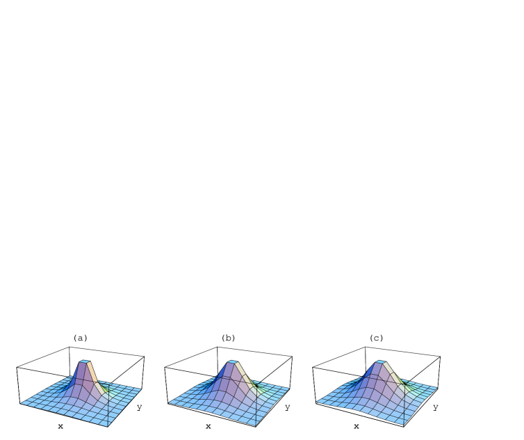
Figure 1: The scalar field (top) and the energy density (bottom) in a plane through the center of the electroweak sphalerons for $(a):M_{H}=\infty$ at $M_{W}L=2.53$, $(b):M_{H}=M_{W}$ and $(c):M_{H}={\scriptstyle{{3\over 4}}}M_{W}$, both at $M_{W}L=4.0$. The energy density is normalized to its peak value (respectively $0.093$, $0.025$ and $0.016M^{4}_{W}/\alpha_{W}$) and the scalar field $\rho$ to its expectation value $v$.

The way we obtained the required configurations was by first constructing a sphaleron for the frozen-length Higgs model, starting at $N=8$. All links at the boundary were first put to the identity, which serves the purpose of positioning the solution in the center of the lattice and of lifting the energy of the finite volume sphaleron by a considerable amount. The latter helps avoid getting trapped in that solution. Centering the energy profile will reduce the probability of getting stuck in a saddle point with spurious unstable modes due to the breakdown of translational and rotational invariance. We then release the frozen boundary condition and compute the Hessian after cooling to verify that we have one unstable mode only. This way the maximal energy density occurs at the center of a plaquette, see fig. 1. The solutions where the maximum occurs at a lattice point are higher in energy. One can now change the lattice spacing in small steps to scan the desired range of parameters. For $N=12$ and 16 the initial configurations were generated from the one at $N=8$, by embedding it in the large lattice (links parallel to the boundary remain constant and those perpendicular to the boundary are put to unity) and adjusting the lattice spacing. For $M_{W}=M_{H}$ we generated the sphalerons for $N=8$ from the frozen-length sphaleron (in not too small a volume) by adding the scalar field, set to its expectation value $v$. Varying the lattice spacing in small steps allows one again to scan the desired range of parameters. Finally, the sphalerons with $M_{H}=0.75M_{W}$ were generated from the ones with $M_{W}=M_{H}$ by simply adjusting the parameters.

$M_{H}=\infty$	$\frac{{\cal E}}{M_{W}/\alpha_{W}}$			$-\frac{\omega^{2}}{M_{W}^{2}}$
$LM_{W}$	$N=8$	$N=12$	$N=16$	$N=8$	$\frac{{\cal E}_{\rm sph}}{M_{W}/\alpha_{W}}$	$\ \frac{{\cal E}_{1}}{M_{W}/\alpha_{W}}$	$\ \frac{{\cal E}_{2}}{M_{W}/\alpha_{W}}$
$2.5298$	$5.2041(2)$	$5.4153(3)$	$5.4699(4)$	$5.846$	$5.525$	$-1.89$	$-13.2$
$2.7713$	$5.0117(1)$	$5.2598(2)$	$5.3258(4)$	$5.442$	$5.395$	$-2.00$	$-9.9$
$2.8823$	$4.9352(1)$	$5.2001(3)$	$5.2728(4)$	$5.325$	$5.351$	$-2.15$	$-8.1$
$2.9933$	$4.8645(1)$	$5.1459(3)$	$5.2263(5)$	$5.250$	$5.316$	$-2.34$	$-6.3$
$3.2000$	$4.7446(1)$	$5.0549(4)$	$5.1535(5)$	$5.231$	$5.273$	$-2.87$	$-2.7$
$\frac{{\cal E}_{\rm sph}(L)}{M_{W}/\alpha_{W}}=5.09(1)+13.6(5)\frac{e^{-M_{W}L}}{M_{W}L},\quad\frac{{\cal E}_{v}}{M_{W}/\alpha_{W}}=5.0707$
$M_{H}=M_{W}$	$\frac{{\cal E}}{M_{W}/\alpha_{W}}$			$-\frac{\omega^{2}}{M_{W}^{2}}$
$LM_{W}$	$N=8$	$N=12$	$N=16$	$N=8$	$\frac{{\cal E}_{\rm sph}}{M_{W}/\alpha_{W}}$	$\ \frac{{\cal E}_{1}}{M_{W}/\alpha_{W}}$	$\ \frac{{\cal E}_{2}}{M_{W}/\alpha_{W}}$
$3.8000$	$3.6564(1)$	$3.7090(1)$	$3.7261(8)$	$2.371$	$3.747$	$-0.36$	$-0.18$
$4.0000$	$3.6249(1)$	$3.6830(1)$	$3.7013(5)$	$2.313$	$3.723$	$-0.34$	$-0.22$
$4.1600$	$3.6026(1)$	$3.6657(1)$	$3.6852(4)$	$2.287$	$3.708$	$-0.33$	$-0.24$
$4.2208$	$3.5946(1)$	$3.6597(2)$	$3.6798(5)$	$2.281$	$3.704$	$-0.33$	$-0.24$
$4.4000$	$3.5724(1)$	$3.6440(1)$	$3.6660(5)$	$2.280$	$3.692$	$-0.33$	$-0.23$
$4.6000$	$3.5490(1)$	$3.6290(1)$	$3.6527(4)$	$2.308$	$3.680$	$-0.31$	$-0.27$
$4.8000$	$3.5258(1)$	$3.6160(1)$	$3.6418(4)$	$2.380$	$3.671$	$-0.29$	$-0.30$
$\frac{{\cal E}_{\rm sph}(L)}{M_{W}/\alpha_{W}}=3.6406(6)+18.1(2)\frac{e^{-M_{W}L}}{M_{W}L},\quad\frac{{\cal E}_{v}}{M_{W}/\alpha_{W}}=3.6417$
$M_{H}={\scriptstyle{{3\over 4}}}M_{W}$	$\frac{{\cal E}}{M_{W}/\alpha_{W}}$			$-\frac{\omega^{2}}{M_{W}^{2}}$
$LM_{W}$	$N=8$	$N=12$	$N=16$	$N=8$	$\frac{{\cal E}_{\rm sph}}{M_{W}/\alpha_{W}}$	$\ \frac{{\cal E}_{1}}{M_{W}/\alpha_{W}}$	$\ \frac{{\cal E}_{2}}{M_{W}/\alpha_{W}}$
$4.0000$	$3.4193(2)$	$3.4578(2)$	$3.4703(4)$	$1.916$	$3.486$	$-0.24$	$-0.11$
$4.4000$	$3.4078(2)$	$3.4585(2)$	$3.4743(3)$	$1.886$	$3.493$	$-0.24$	$-0.15$
$4.8000$	$3.3925(1)$	$3.4584(1)$	$3.4782(3)$	$1.934$	$3.501$	$-0.24$	$-0.17$
$5.2000$	$3.3699(2)$	$3.4565(2)$	$3.4807(3)$	$2.100$	$3.507$	$-0.23$	$-0.23$
$\frac{{\cal E}_{\rm sph}(L)}{M_{W}/\alpha_{W}}=3.530(3)+24(4)\frac{e^{-M_{W}L}}{M_{W}L}-12(2)\frac{e^{-M_{H}L}}{M_{W}L},\quad\frac{{\cal E}_{v}}{M_{W}/\alpha_{W}}=3.5355$

Table 1: Lattice data for the sphaleron energies ${\cal E}$, the negative eigenvalue of the Hessian on a $8^{3}$ lattice, the fit to the lattice spacing dependence, and volume dependence. We give as many digits as we believe to be significant. The variational result is denoted by ${\cal E}_{v}$.

In table 1 we present the results for the sphaleron energies, the negative eigenvalue for the $N=8$ Hessian, the fit to the lattice spacing dependence (eq. (29)) and to the volume dependence (eq. (36)). We list the variational results [5] for ${\cal E}_{\rm sph}^{\infty}$ as ${\cal E}_{v}$. For the frozen-length Higgs model [4] we have here performed some further cooling down to $\hat{S}<10^{-5}M^{3}_{W}/\alpha_{W}$ for $N=16$ (and one or two orders of magnitude smaller for $N=8$ and $12$), to justify the five digit accuracy (estimated errors in the last digit given between brackets). As was to be expected, one finds appreciable lattice artefacts for the case $M_{H}=\infty$. On the other hand they are comfortably small for $M_{H}\approx M_{W}$. To demonstrate this further we also computed at $M_{W}=M_{H}$ and $N=8$ the energies for $aM_{W}=0.644,\,0.663,\,0.788$ and $0.825$ giving respectively ${\cal E}=3.493,\,3.476,\,3.355$ and $3.305M_{W}/\alpha_{W}$. These are solutions with a negative trace for one of the links, as described above, which is why we did not use these values for the finite size scaling. Nevertheless, it shows that even for these rather coarse lattices, the error in the sphaleron energy is only 10%, which was somewhat surprising. For these solutions the lattice artefacts are described well by the fit to the lattice spacing dependence given in the table (at $M_{W}L=4.8$ for $M_{W}=M_{H}$).

Figure 2: Continuum extrapolated values for ${\cal E}_{\rm sph}$ as a function of the physical volume $M_{W}L$, combined with fits to the finite volume behaviour for $(a):M_{H}=\infty$, $(b):M_{H}=M_{W}$ and $(c):M_{H}={\scriptstyle{{3\over 4}}}M_{W}$.

Figure 2 compares the fit to eq. (36) with the continuum extrapolated lattice data. Our results for ${\cal E}_{\rm sph}^{\infty}$ are in very good agreement with the variational analysis [5], particularly for $M_{W}=M_{H}$, where we achieve an accuracy of better than .05%. For $M_{H}=\infty$, a much better fit with ${\cal E}_{\rm sph}^{\infty}=5.075(5)M_{W}/\alpha_{W}$ is obtained when dropping the largest-volume data point. This was the only case where the energy is lowered significantly as compared to ref. [4], seemingly because we are unable to avoid being trapped in saddle points with additional unstable modes at $N\geq 12$. Note that at some point subleading exponential corrections will start to become relevant too. For $M_{H}=M_{W}$, dropping the last point gives ${\cal E}_{\rm sph}^{\infty}=3.6412(8)M_{W}/\alpha_{W}$, whereas for $M_{H}={\scriptstyle{{3\over 4}}}M_{W}$ we find $3.535M_{W}/\alpha_{W}$. The values of $C_{H}^{2}$ and $\cos(2\delta)C_{W}^{2}$ obtained from these fits (cmp. table 1) agree with what one can roughly extract from the figures of ref. [5].

An alternative method for studying the electroweak sphaleron on the lattice is being considered by Ambjørn and Krasnitz, using the Chern-Simons functional to constrain the cooling [12]. It has the advantage of allowing ordinary cooling rather than saddle-point cooling and might also be used for computing the energy along the tunnelling path. In the continuum the sphaleron has a Chern-Simons number of a half (compared to the trivial vacuum). Its disadvantage is that implementing the Chern-Simons functional on a lattice, the electroweak sphaleron will only approximately be characterized by a Chern-Simons number of exactly one half. As the tunnelling rate depends exponentially on the sphaleron energy, our results might be particularly useful in numerical checks of the semiclassical determination [13] of the tunnelling rate at small temperatures [3, 14] (for the Abelian Higgs model in 1+1 dimensions see ref. [15]), as our method gives the exact saddle-point solution for the sphaleron on a lattice.

References

• [1] R. Dashen B. Hasslacher and A. Neveu, Phys.Rev. D10 (1974) 4138
• [2] F. R. Klinkhamer and N. Manton, Phys.Rev. D30 (1984) 2212
• [3] J. AmbjΓΈrn, T. Askgaard, H. Porter and M.E. Shaposhnikov, Nucl.Phys. B353 (1991) 346; M. Shaposhnikov, Nucl.Phys. B(Proc.Suppl.)26 (1992) 78; J. AmbjΓΈrn and A. Krasnitz, Phys.Lett. B362 (1995) 97; For a recent review see: K. Jansen, Status of the Finite Temperature Electroweak Phase Transition on the Lattice, DESY 95-169, hep-lat/9509018
• [4] M. GarcΓ­a PΓ©rez and P. van Baal, Nucl.Phys. B(Proc.Suppl)42 (1995) 575.
• [5] L. Yaffe, Phys.Rev. D40 (1989) 3463; J. Kunz and Y. Brihaye, Phys.Lett. 216B (1989) 353.
• [6] G. Eilam and A. Stern, Nucl.Phys. B294 (1987) 775.
• [7] Review of particle properties, L. Montanet et al., Phys.Rev. D50 (1994) 1173.
• [8] W. Langguth, I. Montvay and P. Weisz, Nucl.Phys. B277 (1986) 11.
• [9] B. Berg, Phys.Lett. 104B (1981) 475; J. Hoek, M. Teper and J. Waterhouse, Nucl.Phys. B288 (1987) 589.
• [10] A. Duncan and R.D. Mawhinney, Nucl.Phys. B(Proc.Suppl.)26 (1992) 444; Phys.Lett. B282 (1992) 423; A.J. van der Sijs, Nucl.Phys. B(Proc.Suppl.)30 (1993) 893; Phys.Lett. B294 (1992) 391.
• [11] M. GarcΓ­a PΓ©rez and P. van Baal, Nucl.Phys. B429 (1994) 451.
• [12] J. AmbjΓΈrn and A. Krasnitz, private communication and work in progress.
• [13] L.Carson, X. Li, L. McLerran, R. Wang, Phys.Rev. D42 (1990) 2127; J. Baacke and S. Junker, Phys.Rev. D49 (1994) 2055 (E: D50 (1994) 4227), and references therein.
• [14] J. Smit and W. Tang, DESY workshop 1995.
• [15] D.Yu. Grigoriev, V.A. Rubakov and M.E. Shaposhnikov, Nucl.Phys. B326 (1989) 737; A.I. Bochkarev and G.G. Tsitsishvili, Phys.Rev. D40 (1989) 1378; A. Krasnitz and R. Potting, Phys.Lett. B318 (1993) 492; P. de Forcrand, A. Krasnitz and R. Potting, Phys.Rev. D50 (1994) 6054; J. Smit and W. Tang, Nucl.Phys. B(Proc.Suppl.)34 (1994) 616; ibid. 42 (1995) 590.