Critical Slowing-Down in
$SU(2)$ Landau Gauge-Fixing Algorithms

Abstract

We study the problem of critical slowing-down for gauge-fixing algorithms (Landau gauge) in $SU(2)$ lattice gauge theory on a $2$-dimensional lattice. We consider five such algorithms, and lattice sizes ranging from $8^{2}$ to $36^{2}$ (up to $64^{2}$ in the case of Fourier acceleration). We measure four different observables and we find that for each given algorithm they all have the same relaxation time within error bars. We obtain that: the so-called Los Alamos method has dynamic critical exponent $z\approx 2$, the overrelaxation method and the stochastic overrelaxation method have $z\approx 1$, the so-called Cornell method has $z$ slightly smaller than $1$ and the Fourier acceleration method completely eliminates critical slowing-down. A detailed discussion and analysis of the tuning of these algorithms is also presented.

1 Introduction

The lattice formulation of QCD provides a regularization which makes the gauge group compact, so that the Gibbs average of any gauge-invariant quantity is well-defined and thus gauge fixing is, in principle, not needed. However, to better understand the relationship between continuum and lattice models, one is led to consider gauge-dependent quantities on the lattice as well, which requires gauge fixing. It is therefore important to devise numerical algorithms to efficiently gauge fix a lattice configuration. The efficiency of these algorithms is even more important if the problem of existence of Gribov copies in the lattice is taken into account [1]–[4]. In fact, since usually it is not clear how an algorithm selects among different Gribov copies, numerical results using gauge fixing could depend on the gauge-fixing algorithm, making their interpretation conceptually difficult. In these cases, in order to analyze the dependence on the Gribov ambiguity [2, 4, 5], several Gribov copies of the same thermalized configuration have to be produced, and therefore gauge fixing is extensively used.

In this paper we study the problem of fixing the standard lattice Landau gauge condition [6, 7]. As we will see in the next section, this condition is formulated as a minimization problem for the energy of a nonlinear $\sigma$-model with disordered couplings. Two basic deterministic local algorithms have been introduced to achieve this goal. Following [8] we will refer to them as the “Los Alamos” method [12, 13] and the “Cornell” method [14]. Both methods are expected to perform poorly [8], especially as the volume of the lattice increases, due to the phenomenon of critical slowing-down, which afflicts Monte Carlo simulations of critical phenomena as well as some deterministic iterative methods, such as our gauge fixing. Roughly speaking, the problem is that, since the updating is local, the “information” travels at each step only from one lattice site to its nearest neighbors, executing a kind of random walk through the lattice; as a result, in order to get any significant change in configuration, we must wait a time of the order of the square of the typical “physical length” of the system, which is in our case the lattice size $N$. More precisely, the relaxation time (measured in sweeps) for conventional local algorithms diverges as the square of the linear size of the system, or equivalently these methods have dynamic critical exponent $z=2$. This $\,N^{2}\,$ behavior is not a serious difficulty for small lattices, and other aspects of the algorithms may be of greater importance in this case; but as one deals with progressively larger lattices (in order to approach the continuum limit) this factor constitutes a severe limitation.

To overcome this problem, two solutions are available: one can either modify the local update, in such a way that the “length” of the move in the configuration space is increased [16], and therefore this space is explored faster, or introduce some kind of global updating, in order to speed up the relaxation of the long-wavelength modes, which are the slow ones. Various methods, based on these two ideas, have been proposed: overrelaxation [16], stochastic overrelaxation [13], multigrid schemes [13, 17, 18, 19], Fourier acceleration [14], wavelet acceleration [20], etc. By analogy with other deterministic problems [9, 10, 11] and with Monte Carlo simulations [21, 22], the “improved” local algorithms (such as overrelaxation and stochastic overrelaxation) are expected to reduce but not eliminate critical slowing-down ($z\approx 1$, as opposed to $z\approx 2$ for conventional methods), while global methods (such as multigrid, Fourier acceleration, etc.) hope to eliminate critical slowing-down completely (i.e., $z=0$). In any case, a precise determination of the dynamic critical exponents for the different algorithms is of great importance, as are analyses and comparisons between the methods applied to the problem at hand. Such analyses have been partially done in some of the references given here, but we feel that systematic studies of these methods for the specific problem of Landau gauge fixing are lacking, especially with regard to the evaluation of dynamic critical exponents, although some of the algorithms we consider were extensively analyzed when applied to other numerical problems. The only algorithm thoroughly studied in the past was the multigrid [3, 13, 18, 19] and we will not consider it here. For our research, we have decided to study, besides the two “basic” algorithms (Los Alamos and Cornell), the standard overrelaxation and the stochastic overrelaxation (both applied to the Los Alamos method), which are very appealing for their simplicity and almost absence of overhead. We will also study the Fourier acceleration (applied to the Cornell method), for which not so many studies have been done up to now, and which is claimed [23] to be the best method available today for Landau gauge fixing.

In this work our goals are:

1. studying the critical slowing-down for the various algorithms and finding accurate values for their dynamic critical exponents,

2. analyzing the relative size of several quantities, usually employed in the literature to test the convergence of the gauge fixing, in order to understand which of them should be used in practical computations,

3. doing, when necessary, a careful tuning of the algorithms, checking the “empirical” formulae commonly used for the optimal choice of the parameters, or finding a simple prescription when this formula is not known,

4. comparing the computational costs of the algorithms,

5. doing a simple analysis of the algorithms in order to get at least an idea of how they deal with the problem of critical slowing-down.

Regarding the last point, we will essentially try to review what is known about the algorithms under analysis. Here, in fact, we are unable to do a more rigorous analysis (in the style of [24] or [25] for the gaussian model), due to the non-linearity of the update and the presence of “random” link-dependent coupling constants.

The paper is organized as follows. In Section 2 we present a pedagogical review of the problem of Landau gauge fixing on the lattice. In particular, to make the analysis of the efficiency of the local algorithms a little more quantitative, we introduce two functions: the variation of the minimizing function at each site $\,\Delta{\widetilde{\cal E}}(\mbox{\boldmath$x$})\,$, and the “length” of the update $\,{\cal D(\mbox{\boldmath$x$})}\,$, interpreted as a move in the configuration space $\{g(\mbox{\boldmath$x$})\}\,$. In Section 3 we define the update for the various algorithms and we explain how each one fights the problem of critical slowing-down. The quantities for which the relaxation time $\tau$ will be measured are introduced in Section 4. In Section 5 the problem of the tuning of the algorithms is addressed, and we try a quantitative analysis to find simple formulae for the optimal choice of the parameters. Finally, in Section 6, we give some more details about the numerical simulations and the computational aspects of our work and, in Section 7, we present our results and conclusions.

The main difficulty we had to overcome in this project was the severe lack of computer time, which restricted us to dealing with the $SU(2)$ gauge group, instead of the more interesting $SU(3)$ case, and with small lattice sizes. On the other hand, the use of $SU(2)$ makes the analysis of the algorithms simpler, and with the values of $\beta$ that we consider (see Section 4) no significant finite-size corrections are expected to occur and the use of small lattices is justified.

A further difficulty is the definition of constant physics, necessary for finding the dynamic critical exponents that characterize each algorithm (see Section 4). This definition is very simple only in dimension $d=2$ and this is the case we will consider here, leaving the extension of this work to four dimensions to a future paper [26].

Nevertheless, we believe that this work presents a comprehensive analysis and comparison of the different methods considered, and enough evidence for the evaluation of their dynamic critical exponents. Our findings for the exponents are basically confirmations of what is generally accepted, with the exception of the value slightly smaller than one for the Cornell method, a fact that we try to interpret in Sections 5 and 7.

The total computer time used in our simulations was about 225 hours on an IBM RS-6000/250 machine.

2 Landau Gauge-Fixing Condition on the Lattice

Let us consider a standard Wilson action for $SU(2)$ lattice gauge theory in $d$ dimensions [27] :

$$S\left(\left\{U\right\}\right)\equiv\frac{4a^{d-4}}{g^{2}_{0}}\,\frac{1}{2}\sum_{\mu,\nu=1}^{d}\,\sum_{\mbox{\boldmath$x$}}\,\biggl{\{}\,1\,-\frac{1}{2}Tr\left[\ U_{\mu}(\mbox{\boldmath$x$})\;U_{\nu}(\mbox{\boldmath$x$}+a\mbox{\boldmath$e$}_{\mu})\;U_{\mu}^{-1}(\mbox{\boldmath$x$}+a\mbox{\boldmath$e$}_{\nu})\;U_{\nu}^{-1}(\mbox{\boldmath$x$})\right]\,\biggr{\}}$$ (2.1)

where $U_{\mu}(\mbox{\boldmath$x$})\in SU(2)$ are the link variables, $g_{0}$ is the bare coupling constant, $a$ is the lattice spacing and $\mbox{\boldmath$e$}_{\mu}$ is a unit vector in the positive $\mu$ direction. Sites are labeled by $d$-dimensional vectors $x$ . The lattice size in the $\mu$ direction is $L_{\mu}\equiv a\,N_{\mu}$ where $N_{\mu}$ is an integer. We assume periodic boundary conditions, i.e. $\mbox{\boldmath$x$}+L_{\mu}\mbox{\boldmath$e$}_{\mu}\equiv\mbox{\boldmath$x$}$, and the lattice volume is given by

$$V\equiv\prod_{\mu=1}^{d}L_{\mu}\,=\,a^{d}\prod_{\mu=1}^{d}N_{\mu}\;\mbox{.}$$ (2.2)

The gauge field is defined as

$$A_{\mu}(\mbox{\boldmath$x$})\,\equiv\,\frac{1}{2ag_{0}}\left[\;U_{\mu}(\mbox{\boldmath$x$})-U_{\mu}^{\dagger}(\mbox{\boldmath$x$})\;\right]\;\mbox{;}$$ (2.3)

this variable approaches the classical gauge potential in the continuum limit.

To fix the Landau gauge we look for a local minimum of the function [6, 7]

$${\cal E}\left(\left\{g\right\}\right)\;\equiv\;1-\frac{a^{d}}{2\,d\,V}\sum_{\mu=1}^{d}\sum_{\mbox{\boldmath$x$}}\,\frac{1}{2}\,\mbox{Tr}\left[\;U_{\mu}^{\left(g\right)}(\mbox{\boldmath$x$})+U_{\mu}^{\left(g\right)\dagger}(\mbox{\boldmath$x$})\;\right]$$ (2.4)

keeping the configuration $\left\{U_{\mu}(\mbox{\boldmath$x$})\right\}$ fixed. Here each $\,g(\mbox{\boldmath$x$})\in SU(2)\,$ is a site variable, $\,{\cal G}\equiv\left\{g(\mbox{\boldmath$x$})\right\}\,$ is a gauge transformation, and $\,U_{\mu}^{\left(g\right)}(\mbox{\boldmath$x$})\,$ is given by

$$U_{\mu}(\mbox{\boldmath$x$})\;\rightarrow\;U_{\mu}^{\left(g\right)}(\mbox{\boldmath$x$})\;\equiv\;g(\mbox{\boldmath$x$})\;U_{\mu}(\mbox{\boldmath$x$})\;g^{\dagger}(\mbox{\boldmath$x$}+a\mbox{\boldmath$e$}_{\mu})\;\mbox{.}$$ (2.5)

We use the following parametrization for the matrices $U\in SU(2)$:

$$U\,\equiv\,u_{0}\,1\!\!\!\bot+i\vec{\mbox{$u$}}\cdot\vec{\mbox{$\sigma$}}\,=\,\left(\begin{array}[]{cc}u_{0}+iu_{3}&u_{2}+iu_{1}\\ -u_{2}+iu_{1}&u_{0}-iu_{3}\end{array}\right)$$ (2.6)

where $1\!\!\!\bot$ is the $2\times 2$ identity matrix, the components of $\vec{\mbox{$\sigma$}}\equiv(\sigma^{1}\mbox{,}\,\sigma^{2}\mbox{,}\,\sigma^{3})$ are the Pauli matrices, $u_{0}\in\hbox{\specialroman R}$, $\vec{\mbox{$u$}}\in\hbox{\specialroman R}^{3}$ and $\,u_{0}^{2}+\vec{\mbox{$u$}}\cdot\vec{\mbox{$u$}}=1$. Therefore

$$U^{-1}=U^{\dagger}=u_{0}\,1\!\!\!\bot-i\,\vec{\mbox{$u$}}\cdot\vec{\mbox{$\sigma$}}$$ (2.7)

and from equations (2.6) and (2.7) it follows that

$$\mbox{Tr}\;U=\mbox{Tr}\;U^{\dagger}=2\,u_{0}\;\mbox{.}$$ (2.8)

By using equations (2.7) and (2.8) we can also write

$$U^{-1}=U^{\dagger}=1\!\!\!\bot\mbox{Tr}\,U-U\;\mbox{.}$$ (2.9)

If $V=v_{0}+i\,\vec{\mbox{$v$}}\cdot\vec{\mbox{$\sigma$}}$ is another $SU(2)$ matrix then, again using (2.6) and (2.7), we obtain

$$\frac{1}{2}\mbox{Tr}\;(\,U\;V^{\dagger}\,) = u_{0}\,v_{0}\,+\,\vec{\mbox{$u$}}\cdot\vec{\mbox{$v$}}$$ (2.10)

$$= u\cdot v\;\mbox{,}$$ (2.11)

where the last step follows if we interpret a matrix $U\in SU(2)$ as a four-dimensional unit vector $u\equiv(u_{0}\mbox{,}\,\vec{\mbox{$u$}})$. Finally, if $U\in SU(2)$, the matrix

$$A\equiv\frac{1}{2}\,[\;U-U^{\dagger}\;]$$ (2.12)

belongs to the $\hbox{\german su}\,(2)$ Lie algebra and is parametrized as

$$A=\,i\,\vec{\mbox{$u$}}\cdot\vec{\mbox{$\sigma$}}=\left(\begin{array}[]{cc}iu_{3}&u_{2}+iu_{1}\\ -u_{2}+iu_{1}&-iu_{3}\end{array}\right)\;\mbox{.}$$ (2.13)

This matrix is traceless, anti-hermitian and

$$\mbox{Tr}\,(\,AA^{\dagger}\,)=\mbox{Tr}\,(\,-A^{2}\,)=2\;\vec{\mbox{$u$}}\cdot\vec{\mbox{$u$}}\;\mbox{.}$$ (2.14)

Let us now consider a one-parameter subgroup $g(\tau;\mbox{\boldmath$x$})$ of $SU(2)$ defined by

$$g(\tau;\mbox{\boldmath$x$})\equiv\exp\left[\;\tau\,\gamma(\mbox{\boldmath$x$})\;\right]$$ (2.15)

where the parameter $\tau$ is a real number and the $\gamma$’s are fixed elements of the $\hbox{\german su}\,(2)$ Lie algebra given by

$$\gamma(\mbox{\boldmath$x$})\,\equiv\,i\,\vec{\mbox{$\gamma$}}(\mbox{\boldmath$x$})\cdot\vec{\mbox{$\sigma$}}$$ (2.16)

with $\vec{\mbox{$\gamma$}}(\mbox{\boldmath$x$})\in\hbox{\specialroman R}^{3}$ for all $x$. Then, for fixed $\{U_{\mu}\left(\mbox{\boldmath$x$}\right)\}$, the minimizing function ${\cal E}$ can be regarded as a function of the parameter $\tau$, and its first derivative is given by the well-known expression

$${\cal E}^{{}^{\prime}}(0)\,=\,\frac{a^{d+2}g_{0}}{d\,V}\,\sum_{\mbox{\boldmath$x$}}\,\left[\gamma(\mbox{\boldmath$x$})\right]_{j}\,\left[\left(\nabla\cdot A^{\left(g\right)}\right)(\mbox{\boldmath$x$})\right]_{j}\;\mbox{,}$$ (2.17)

where the sum in the color index $j$ is understood $(j=1,2,3)$ and

$$\left[\left(\nabla\cdot A\right)(\mbox{\boldmath$x$})\right]_{j}\equiv\frac{1}{a}\sum_{\mu=1}^{d}\,\left[A_{\mu}(\mbox{\boldmath$x$})-A_{\mu}(\mbox{\boldmath$x$}-a\mbox{\boldmath$e$}_{\mu})\right]_{j}$$ (2.18)

is the lattice divergence of

$$\left[A_{\mu}(\mbox{\boldmath$x$})\right]_{j}\,\equiv\,\frac{1}{2\,i}\,\mbox{Tr}\left[A_{\mu}(\mbox{\boldmath$x$})\,\sigma^{j}\right]\;\mbox{.}$$ (2.19)

If $\{U_{\mu}\left(\mbox{\boldmath$x$}\right)\}$ is a stationary point of ${\cal E}(\tau)$ at $\tau=0$ (i.e. $g(\tau,\mbox{\boldmath$x$})=1\!\!\!\bot,\forall\mbox{\boldmath$x$}$) then we have ${\cal E}^{{}^{\prime}}(0)=0$ for all $\{\gamma_{j}(\mbox{\boldmath$x$})\}$. This implies

$$\left[\left(\nabla\cdot A\right)(\mbox{\boldmath$x$})\right]_{j}=0\qquad\qquad\forall\;\;\;\mbox{\boldmath$x$}\mbox{,}\;\;j$$ (2.20)

which is the lattice formulation of the usual local Landau gauge-fixing condition in the continuum. By summing equation (2.20) over the components $x_{\mu}$ of $x$ with $\mu\neq\nu$ and using the periodicity of the lattice, it is easy to check that [7] if the Landau gauge-fixing condition is satisfied then the quantities

$$Q_{\nu}(x_{\nu})\,\equiv\,\sum_{\mu\neq\nu}\,\sum_{x_{\mu}}\,A_{\nu}(\mbox{\boldmath$x$})\qquad\qquad\phantom{forall}\;\;\;\nu=1\mbox{,}\ldots\,\mbox{,}d$$ (2.21)

are constant, i.e. independent of $x_{\nu}$. From this it immediately follows that the longitudinal gluon propagator at zero three-momentum

$$D_{\nu\nu}(x_{\nu}) \equiv \sum_{\mu\neq\nu}\,\sum_{x_{\mu}}\,\frac{1}{2}\,\mbox{Tr}\,\langle\,A_{\nu}(\mbox{\boldmath$x$})\,A_{\nu}(0)\,\rangle$$ (2.22)

$$= \frac{1}{2}\,\mbox{Tr}\,\langle\,Q_{\nu}(x_{\nu})\,A_{\nu}(0)\,\rangle$$ (2.23)

is also constant.

The numerical problem we have to solve is therefore the following: for a given (i.e. fixed) thermalized lattice configuration $\{U_{\mu}(\mbox{\boldmath$x$})\}$, we want to find a gauge transformation $\{g(\mbox{\boldmath$x$})\}$ which brings the function

$${\cal E}\left(\left\{g\right\}\right) = 1\,-\,\frac{a^{d}}{2\,d\,V}\sum_{\mu=1}^{d}\sum_{\mbox{\boldmath$x$}}\,\mbox{Tr}\;U_{\mu}^{\left(g\right)}(\mbox{\boldmath$x$})$$ (2.24)

$$= 1\,-\,\frac{a^{d}}{2\,d\,V}\sum_{\mu=1}^{d}\sum_{\mbox{\boldmath$x$}}\,\mbox{Tr}\left[\;g(\mbox{\boldmath$x$})\;U_{\mu}(\mbox{\boldmath$x$})\;g^{\dagger}(\mbox{\boldmath$x$}+a\mbox{\boldmath$e$}_{\mu})\;\right]$$

to a local minimum, starting from a configuration $g(\mbox{\boldmath$x$})=1\!\!\!\bot$ for all $x$. In order to achieve this result it is sufficient to find an iterative process which, from one iteration step to the next, decreases the value of the minimizing function monotonically (descent methods). In fact, since ${\cal E}$ has a lower bound of 0 (and an upper bound of 2), an algorithm of this kind is expected to converge.

To find a simple iterative algorithm which minimizes ${\cal E}$ one may choose to update a single site variable $g(\mbox{\boldmath$y$})$ at a time. In this case the minimizing function ${\cal E}$ becomes

$${\widetilde{\cal E}}\left[g(\mbox{\boldmath$y$})\right] = constant\,-\,\frac{a^{d}}{2\,d\,V}\,\mbox{Tr}\,w(\mbox{\boldmath$y$})$$ (2.25)

where

$$w(\mbox{\boldmath$y$})\;\equiv\;g(\mbox{\boldmath$y$})\,h(\mbox{\boldmath$y$})$$ (2.26)

and the “single-site effective magnetic field” $\,h(\mbox{\boldmath$y$})\,$ is given by

$$h(\mbox{\boldmath$y$})\equiv\,\sum_{\mu=1}^{d}\left[\;U_{\mu}(\mbox{\boldmath$y$})\;g^{\dagger}(\mbox{\boldmath$y$}+a\mbox{\boldmath$e$}_{\mu})+U_{\mu}^{\dagger}(\mbox{\boldmath$y$}-a\mbox{\boldmath$e$}_{\mu})\;g^{\dagger}(\mbox{\boldmath$y$}-a\mbox{\boldmath$e$}_{\mu})\;\right]\;\mbox{.}$$ (2.27)

The matrices $h(\mbox{\boldmath$y$})$ and $w(\mbox{\boldmath$y$})$ are proportional to $SU(2)$ matrices, namely they can be written as

$$h(\mbox{\boldmath$y$}) \equiv \sqrt{\det h(\mbox{\boldmath$y$})}\;{\widetilde{h}}(\mbox{\boldmath$y$})$$ (2.28)

$$w(\mbox{\boldmath$y$}) \equiv \sqrt{\det w(\mbox{\boldmath$y$})}\;{\widetilde{w}}(\mbox{\boldmath$y$})$$ (2.29)

with ${\widetilde{h}}(\mbox{\boldmath$y$}),{\widetilde{w}}(\mbox{\boldmath$y$})\in SU(2)$ and

$${\cal N}(\mbox{\boldmath$y$})\,\equiv\,\sqrt{\det h(\mbox{\boldmath$y$})}\,=\,\sqrt{\det w(\mbox{\boldmath$y$})}\;\mbox{.}$$ (2.30)

Let us also define

$${\cal T}(\mbox{\boldmath$y$})\equiv\mbox{Tr}\,{\widetilde{w}}(\mbox{\boldmath$y$})\,=\,\mbox{Tr}\,w(\mbox{\boldmath$y$})\,/\,{\cal N}(\mbox{\boldmath$y$})\;\mbox{.}$$ (2.31)

We want to consider the single site update $g(\mbox{\boldmath$y$})\,\rightarrow\,g^{(new)}(\mbox{\boldmath$y$})\,$, which can alternatively be looked at as the multiplicative update

$$g(\mbox{\boldmath$y$})\,\rightarrow\,g^{(new)}(\mbox{\boldmath$y$})\equiv R^{(update)}(\mbox{\boldmath$y$})\,g(\mbox{\boldmath$y$})\;\mbox{,}$$ (2.32)

with $R^{(update)}(\mbox{\boldmath$y$})\in SU(2)$. Under this update, the variation of the minimizing function is given by

$$\Delta{\widetilde{\cal E}}(\mbox{\boldmath$y$}) = \frac{a^{d}{\cal N}(\mbox{\boldmath$y$})}{2\,d\,V}\,\mbox{Tr}\,\biggl{\{}\left[\;g(\mbox{\boldmath$y$})\,-\,g^{(new)}(\mbox{\boldmath$y$})\;\right]{\widetilde{h}}(\mbox{\boldmath$y$})\biggr{\}}$$ (2.33)

$$= \frac{a^{d}{\cal N}(\mbox{\boldmath$y$})}{2\,d\,V}\,\mbox{Tr}\,\biggl{\{}\left[\;1\,-\,R^{(update)}(\mbox{\boldmath$y$})\;\right]{\widetilde{w}}(\mbox{\boldmath$y$})\biggr{\}}\;\mbox{.}$$ (2.34)

To measure the length of the move $g(\mbox{\boldmath$y$})\,\rightarrow\,g^{(new)}(\mbox{\boldmath$y$})$ we can use the quantity [28]

$${\cal D}\left[g(\mbox{\boldmath$y$}),\,g^{(new)}(\mbox{\boldmath$y$})\right]\equiv\,\;{\cal D}(\mbox{\boldmath$y$}) \equiv \sqrt{\,\frac{1}{2}\,\mbox{Tr}\,\biggl{\{}\left[\,g(\mbox{\boldmath$y$})-g^{(new)}(\mbox{\boldmath$y$})\,\right]\left[\,g(\mbox{\boldmath$y$})-g^{(new)}(\mbox{\boldmath$y$})\,\right]^{\dagger}\biggr{\}}\,}$$ (2.35)

$$= \sqrt{\,2\,-\,\mbox{Tr}\,\left[\,g^{(new)}(\mbox{\boldmath$y$})\,g^{\dagger}(\mbox{\boldmath$y$})\,\right]\,}$$

$$= \sqrt{\,2\,-\,\mbox{Tr}\,R^{(update)}(\mbox{\boldmath$y$})\,}$$

which satisfies the defining properties of a distance function for any set of matrices and, if we interpret $SU(2)$ matrices as four-dimensional unit vectors, it coincides with the standard euclidean distance in $\hbox{\specialroman R}^{4}\,$ [see formula (2.11)].

In the next section the local quantities $\,\Delta{\widetilde{\cal E}}(\mbox{\boldmath$y$})\,$ and $\,{\cal D}(\mbox{\boldmath$y$})\,$ will be used to illustrate the performance of the different local methods considered. In particular, their expressions will be written completely in terms of the tuning parameter for the algorithm (if needed), the square root $\,{\cal N}(\mbox{\boldmath$y$})\,$ of the determinant of $w(\mbox{\boldmath$y$})$ and $h(\mbox{\boldmath$y$})$, and the trace $\,{\cal T}(\mbox{\boldmath$y$})\,$ of the normalized matrix $\,{\widetilde{w}}(\mbox{\boldmath$y$})\,$.

3 The Algorithms

In this section we will describe the five algorithms for which we want to analyze the critical slowing-down. In particular, we will compare the implementation and performance of the four local algorithms considered in Sections 3.1–3.4, by comparing their expressions for the quantities $\,\Delta{\widetilde{\cal E}}(\mbox{\boldmath$y$})\,$ and $\,{\cal D}(\mbox{\boldmath$y$})\,$ introduced in the previous section.

As explained before, $\,\Delta{\widetilde{\cal E}}(\mbox{\boldmath$y$})\,$ measures by how much the “local energy” is reduced in a single step of the algorithm at site $y$, while $\,{\cal D}(\mbox{\boldmath$y$})\,$ measures by how much the configuration at site $y$ was effectively changed. Therefore they represent the two (possibly conflicting) tasks that a local algorithm is expected to perform: minimizing the energy at every site and at the same time moving efficiently through the configuration space.

As we will see in Section 3.1 below, the Los Alamos method has the “best” possible value for $\,\Delta{\widetilde{\cal E}}(\mbox{\boldmath$y$})\,$, i.e. it brings the “single site energy” to its absolute minimum in one iteration. We take the Los Alamos method as a basis for comparing all the other local algorithms we consider, which will typically have smaller $\,\Delta{\widetilde{\cal E}}(\mbox{\boldmath$y$})\,$ (in magnitude) and larger $\,{\cal D}(\mbox{\boldmath$y$})\,$ than the Los Alamos method, and will perform better.

In order to make this comparison more quantitative we will also look at the ratios

$${\cal R}_{{\cal E}}(\mbox{\boldmath$y$})\equiv\frac{\Delta{\widetilde{\cal E}}^{(LosAl.)}(\mbox{\boldmath$y$})\,-\,\Delta{\widetilde{\cal E}}(\mbox{\boldmath$y$})}{\Delta{\widetilde{\cal E}}^{(LosAl.)}(\mbox{\boldmath$y$})}$$ (3.1)

and

$${\cal R}_{{\cal D}}(\mbox{\boldmath$y$})\equiv\frac{{\cal D}(\mbox{\boldmath$y$})\,-\,{\cal D}^{(LosAl.)}(\mbox{\boldmath$y$})}{{\cal D}^{(LosAl.)}(\mbox{\boldmath$y$})}$$ (3.2)

for the various methods. They measure, respectively, the relative “loss” in minimizing ${\widetilde{\cal E}}(\mbox{\boldmath$y$})\,$ and the relative “gain” in the length of the update, when compared with the Los Alamos method. In the next subsections these two quantities will be evaluated, for each local algorithm, as functions of $\,{\cal N}(\mbox{\boldmath$y$})\,$ and $\,{\cal T}(\mbox{\boldmath$y$})\,$ (defined in the previous section) and the tuning parameter. In particular, their limits as $\,{\cal T}(\mbox{\boldmath$y$})\,\to 2$ will be computed. In fact, as discussed in Section 5, these limits are useful to point out analogies between the algorithms and compare their efficiencies in fighting critical slowing-down.

3.1 Los Alamos Method

It is easy to see from equations (2.33) and (2.34) that the choice [12, 13]

$$g^{(new)}(\mbox{\boldmath$y$})\,=\,g^{(LosAl.)}(\mbox{\boldmath$y$})\equiv{\widetilde{h}}^{\dagger}(\mbox{\boldmath$y$})\;\mbox{,}$$ (3.3)

or

$$R^{(update)}(\mbox{\boldmath$y$})\,\equiv\,{\widetilde{w}}^{\dagger}(\mbox{\boldmath$y$})\;\mbox{,}$$ (3.4)

gives the maximum negative variation of ${\widetilde{\cal E}}$:

$$\Delta{\widetilde{\cal E}}^{(LosAl.)}(\mbox{\boldmath$y$})\,=\,\frac{a^{d}{\cal N}(\mbox{\boldmath$y$})}{2\,d\,V}\,\left[\,{\cal T}(\mbox{\boldmath$y$})-2\,\right]\leq 0\;\mbox{,}$$ (3.5)

where $\,{\cal T}(\mbox{\boldmath$y$})\,$ was defined in equation (2.31). In other words, the move from $g(\mbox{\boldmath$y$})$ to $g^{(LosAl.)}(\mbox{\boldmath$y$})$ brings the function ${\widetilde{\cal E}}\left[g(\mbox{\boldmath$y$})\right]$ to its unique absolute minimum. For this update we have, from equation (2.35),

$${\cal D}^{(LosAl.)}(\mbox{\boldmath$y$})\,=\,\sqrt{2\,-\,{\cal T}(\mbox{\boldmath$y$})}\;\mbox{.}$$ (3.6)

3.2 Cornell Method

Another possible choice for $\,R^{(update)}(\mbox{\boldmath$y$})\,$ comes from considering an update of the form (2.15) with $\tau=\alpha$ and $\gamma(\mbox{\boldmath$y$})=-a^{2}g_{0}\left(\nabla\cdot A^{\left(g\right)}\right)(\mbox{\boldmath$y$})$. Then, from equation (2.17) we obtain

$$\Delta{\widetilde{\cal E}}\left[g(\mbox{\boldmath$y$})\right]\,=\,-\alpha\frac{a^{d+4}g^{2}_{0}}{d\,V}\,\sum_{j=1}^{3}\,\left[\left(\nabla\cdot A^{\left(g\right)}\right)(\mbox{\boldmath$y$})\right]^{2}_{j}\;+\,{\cal O}(\alpha^{2})$$ (3.7)

and it is clear that the minimizing function decreases if $\alpha$ is small and positive. So we can define [14]

$$R^{(update)}(\mbox{\boldmath$y$})\,\equiv\,\exp\left[-\alpha\,a^{2}\,g_{0}\,\left(\nabla\cdot A^{\left(g\right)}\right)(\mbox{\boldmath$y$})\right]\;.$$ (3.8)

Since we expect $\,a^{2}\,g_{0}\,\left(\nabla\cdot A^{\left(g\right)}\right)(\mbox{\boldmath$y$})\,$ to go to zero as the number of iterations increases, we can expand $\,R^{(update)}(\mbox{\boldmath$y$})\,$ to first order obtaining

$$R^{(update)}(\mbox{\boldmath$y$})\,\propto\,\left[1\!\!\!\bot-\alpha\,a^{2}\,g_{0}\,\left(\nabla\cdot A^{\left(g\right)}\right)(\mbox{\boldmath$y$})\right]\;\mbox{;}$$ (3.9)

here $\propto$ indicates that the matrix on the l.h.s. is proportional to the one on the r.h.s. (namely it has to be reunitarized) and the parameter $\alpha$ is a positive real number which has to be properly tuned, depending on the considered configuration, as discussed below.

If we notice that the matrix $w(\mbox{\boldmath$y$})$ [defined in (2.26)] satisfies the relation

$$w(\mbox{\boldmath$y$})=w^{\dagger}(\mbox{\boldmath$y$})\,+\,2\,a^{2}\,g_{0}\,\left(\nabla\cdot A^{\left(g\right)}\right)(\mbox{\boldmath$y$})$$ (3.10)

we can rewrite equation (3.9) as

$$R^{(update)}(\mbox{\boldmath$y$})\,\propto\,1\!\!\!\bot+\frac{\alpha}{2}\,\left[\,w^{\dagger}(\mbox{\boldmath$y$})\,-w(\mbox{\boldmath$y$})\,\right]$$ (3.11)

and, by using equation (2.9) with $U=w^{\dagger}(\mbox{\boldmath$y$})\,$, we obtain

$$R^{(update)}(\mbox{\boldmath$y$})\,\propto\,\left[1\,-\,\frac{\alpha}{2}\,\mbox{Tr}\,w^{\dagger}(\mbox{\boldmath$y$})\,\right]\,1\!\!\!\bot\,+\,\alpha\,w^{\dagger}(\mbox{\boldmath$y$})\;\mbox{.}$$ (3.12)

Finally, reunitarizing $R^{(update)}(\mbox{\boldmath$y$})$ and using (2.32) we have

$$g^{(new)}(\mbox{\boldmath$y$})\,=\,g^{(cornell)}(\mbox{\boldmath$y$})\,\equiv\,\frac{\alpha\,{\cal N}(\mbox{\boldmath$y$})\,{\widetilde{w}}^{\dagger}(\mbox{\boldmath$y$})\,+\,\left[1\,-\,\alpha\,{\cal N}(\mbox{\boldmath$y$})\,{\cal T}(\mbox{\boldmath$y$})/2\,\right]\,1\!\!\!\bot}{\sqrt{\,1+\alpha^{2}\,{\cal N}^{2}(\mbox{\boldmath$y$})\left[\,1-{\cal T}^{2}(\mbox{\boldmath$y$})/4\,\right]}}\,g(\mbox{\boldmath$y$})\;\mbox{,}$$ (3.13)

where ${\widetilde{w}}(\mbox{\boldmath$y$})$, ${\cal N}(\mbox{\boldmath$y$})$ and ${\cal T}(\mbox{\boldmath$y$})$ are defined respectively in (2.29), (2.30) and (2.31). In this case the variation of the minimizing function is given by

$$\Delta{\widetilde{\cal E}}^{(cornell)}(\mbox{\boldmath$y$})=\frac{a^{d}{\cal N}(\mbox{\boldmath$y$})}{2\,d\,V}\,\left\{\;{\cal T}(\mbox{\boldmath$y$})\,-\,\frac{2\,\alpha\,{\cal N}(\mbox{\boldmath$y$})\,+\,\left[1\,-\,\alpha\,{\cal N}(\mbox{\boldmath$y$})\,{\cal T}(\mbox{\boldmath$y$})/2\,\right]\,{\cal T}(\mbox{\boldmath$y$})}{\sqrt{\,1+\alpha^{2}\,{\cal N}^{2}(\mbox{\boldmath$y$})\left[\,1-{\cal T}^{2}(\mbox{\boldmath$y$})/4\,\right]}}\;\right\}\;\mbox{.}$$ (3.14)

Since ${\cal T}(\mbox{\boldmath$y$})$ is in the interval $[-2,\,2]$ and $\alpha$ is positive this quantity is negative or zero iff $\alpha\,{\cal N}(\mbox{\boldmath$y$})\in(0,\,2]$. Therefore the algorithm converges only if $\alpha$ is positive and small enough. On the other hand, if we evaluate the length of the move $g(\mbox{\boldmath$y$})\,\rightarrow\,g^{(cornell)}(\mbox{\boldmath$y$})$ we obtain from equation (2.35)

$${\cal D}^{(cornell)}(\mbox{\boldmath$y$})\,=\,\sqrt{2}\,\left(1-\left\{1+\alpha^{2}\,{\cal N}^{2}(\mbox{\boldmath$y$})\left[\,1-\frac{{\cal T}^{2}(\mbox{\boldmath$y$})}{4}\,\right]\right\}^{-1/2}\,\right)^{1/2}\;\mbox{;}$$ (3.15)

namely $\alpha$ should not be too small otherwise this length goes to zero.

It is easy to check that in the limit of $\,{\cal T}(\mbox{\boldmath$y$})\to 2\,$ we get for the ratios $\,{\cal R}_{{\cal E}}(\mbox{\boldmath$y$})\,$ and $\,{\cal R}_{{\cal D}}(\mbox{\boldmath$y$})\,$ [defined respectively in (3.1) and (3.2)]

$${\cal R}^{(Cornell)}_{{\cal E}}(\mbox{\boldmath$y$})\,\rightarrow\,\left[\,\alpha\,{\cal N}(\mbox{\boldmath$y$})\,-\,1\,\right]^{2}$$ (3.16)

and

$${\cal R}^{(Cornell)}_{{\cal D}}(\mbox{\boldmath$y$})\,\rightarrow\,\left[\,\alpha\,{\cal N}(\mbox{\boldmath$y$})\,-\,1\,\right]\;\mbox{.}$$ (3.17)

Therefore, as $\,{\cal T}(\mbox{\boldmath$y$})\,$ approaches $2$ we have that, at least for the case $\,1<\alpha\,{\cal N}(\mbox{\boldmath$y$})<2\,$, the gain in the length of the move with respect to the Los Alamos method is linear in $\,\left[\,\alpha\,{\cal N}(\mbox{\boldmath$y$})\,-\,1\,\right]\,$, while the loss in the minimizing of the energy is quadratically small. This illustrates why the algorithm will perform better than the Los Alamos method. For further discussion, see Section 5.

3.3 Overrelaxation Method

The standard overrelaxation method [16] is a local algorithm in which, instead of using the update

$$g(\mbox{\boldmath$y$})\,\rightarrow\,g^{(LosAl.)}(\mbox{\boldmath$y$})={\widetilde{w}}^{\dagger}(\mbox{\boldmath$y$})\,g(\mbox{\boldmath$y$})$$ (3.18)

described in Section 3.1, we use the substitution

$$g(\mbox{\boldmath$y$})\,\rightarrow\,g^{(new)}(\mbox{\boldmath$y$})\,=\,g^{(over)}(\mbox{\boldmath$y$})\equiv\left[\,{\widetilde{w}}^{\dagger}(\mbox{\boldmath$y$})\,\right]^{\omega}\,g(\mbox{\boldmath$y$})\;\mbox{,}$$ (3.19)

where the overrelaxation parameter $\omega$ varies in the interval $\,1<\omega<2\,$ and has an optimal value which is volume- and problem-dependent. Of course, for $\omega=1$, we have $g^{(over)}(\mbox{\boldmath$y$})=g^{(LosAl.)}(\mbox{\boldmath$y$})$ while, for $\omega=2$, we obtain

$$g^{(over)}(\mbox{\boldmath$y$})\,=\,{\widetilde{w}}^{\dagger}(\mbox{\boldmath$y$})\,{\widetilde{w}}^{\dagger}(\mbox{\boldmath$y$})\,g(\mbox{\boldmath$y$})\;\mbox{,}$$ (3.20)

and it is easy to check that [see equation (2.34)]

$$\Delta{\widetilde{\cal E}}(\mbox{\boldmath$y$})\;=\;\frac{a^{d}{\cal N}(\mbox{\boldmath$y$})}{2\,d\,V}\,\mbox{Tr}\,\left[\;{\widetilde{w}}(\mbox{\boldmath$y$})\,-\,{\widetilde{w}}^{\dagger}(\mbox{\boldmath$y$})\;\right]\;=\;0\;\mbox{,}$$ (3.21)

namely for $\omega=2$ the algorithm does not converge, as the energy is never decreased.

Finally, for $1<\omega<2$, we can write

$$g^{(over)}(\mbox{\boldmath$y$})=\left[\,{\widetilde{w}}^{\dagger}(\mbox{\boldmath$y$})\,\right]^{\omega-1}g^{(LosAl.)}(\mbox{\boldmath$y$})\;\mbox{.}$$ (3.22)

Therefore we can interpret this update as a move from $g(\mbox{\boldmath$y$})$ to $g^{(over)}(\mbox{\boldmath$y$})$ “passing through” $g^{(LosAl.)}(\mbox{\boldmath$y$})$. In this way, the minimizing function ${\widetilde{\cal E}}\left[g(\mbox{\boldmath$y$})\right]$ will not go to its absolute minimum, even though its variation $\Delta{\widetilde{\cal E}}$ will still be negative. For computing $\left[\,{\widetilde{w}}^{\dagger}(\mbox{\boldmath$y$})\,\right]^{\omega}$ one uses the binomial expansion

$$\left[\,{\widetilde{w}}^{\dagger}(\mbox{\boldmath$y$})\,\right]^{\omega}\,=\,\sum_{n=0}^{\infty}\,\frac{\Gamma(\omega+1)}{n!\;\Gamma(\omega+1-n)}\,\left[\,{\widetilde{w}}^{\dagger}(\mbox{\boldmath$y$})-1\!\!\!\bot\,\right]^{n}\;\mbox{.}$$ (3.24)

Since the matrix ${\widetilde{w}}^{\dagger}(\mbox{\boldmath$y$})$ is expected to converge to the identity matrix $1\!\!\!\bot$, this series can be truncated after a few terms, followed by reunitarization of the resulting matrix; for example, if only two terms are kept, we have

$$g^{(over)}(\mbox{\boldmath$y$})\,=\,\frac{\biggl{\{}1\!\!\!\bot+\omega\left[\,{\widetilde{w}}^{\dagger}(\mbox{\boldmath$y$})-1\!\!\!\bot\,\right]\,\biggr{\}}}{\sqrt{1+\omega\left(\omega-1\right)\left[\,2-{\cal T}(\mbox{\boldmath$y$})\,\right]}}\,g(\mbox{\boldmath$y$})\;\mbox{.}$$ (3.25)

In this way the variation of the minimizing function is given by [ see equation (2.34) ]

$$\Delta{\widetilde{\cal E}}^{(over)}(\mbox{\boldmath$y$})\,=\,\frac{a^{d}{\cal N}(\mbox{\boldmath$y$})}{2\,d\,V}\,\left\{\;{\cal T}(\mbox{\boldmath$y$})\,-\,\frac{\left(1-\omega\right){\cal T}(\mbox{\boldmath$y$})\,+\,2\,\omega}{\sqrt{1+\omega\left(\omega-1\right)\left[\,2-{\cal T}(\mbox{\boldmath$y$})\,\right]}}\;\right\}\;\mbox{.}$$ (3.26)

Since $\,{\cal T}(\mbox{\boldmath$y$})\in[-2,2]$ and $\omega\in(1,2)$ it is easy to check that this variation is always negative or zero. The length of the move [formula (2.35)] is given by

$${\cal D}^{(over)}(\mbox{\boldmath$y$})\,=\,\left\{\,2-\frac{2-\,\omega\left[\,2\,-\,{\cal T}(\mbox{\boldmath$y$})\,\right]}{\sqrt{1+\omega\left(\omega-1\right)\left[\,2-{\cal T}(\mbox{\boldmath$y$})\,\right]}}\right\}^{1/2}\;\mbox{.}$$ (3.27)

As an illustration of the improvement with respect to the Los Alamos method, let us consider $\omega$ slightly larger than $1$. Expanding the expressions for $\,\Delta{\widetilde{\cal E}}^{(over)}\,$ and $\,{\cal D}^{(over)}\,$ around $\,\omega=1$, we obtain

$$\Delta{\widetilde{\cal E}}^{(over)}(\mbox{\boldmath$y$})\,=\,\frac{a^{d}{\cal N}(\mbox{\boldmath$y$})}{2\,d\,V}\,\left[\,{\cal T}(\mbox{\boldmath$y$})\,-\,2\,\right]\,\left\{\,1\,-\frac{1}{4}\left(\omega-1\right)^{2}\,\left[\,2+{\cal T}(\mbox{\boldmath$y$})\,\right]\,+\,{\cal O}\left(\left(\omega-1\right)^{3}\right)\,\right\}$$ (3.28)

and

$${\cal D}^{(over)}(\mbox{\boldmath$y$})\,=\,\sqrt{\,2-{\cal T}(\mbox{\boldmath$y$})\,}\,\left\{\,1+\frac{1}{4}\left(\omega-1\right)\,\left[\,2+{\cal T}(\mbox{\boldmath$y$})\,\right]\,+\,{\cal O}\left(\left(\omega-1\right)^{2}\right)\,\right\}\;\mbox{,}$$ (3.29)

namely the correction with respect to the variation (3.5) is positive and quadratic in $(\omega-1)$, while the correction with respect to the length (3.6) is positive and linear in $(\omega-1)$. Thus, already for a value of $\omega$ slightly larger than one, what we lose in minimizing ${\widetilde{\cal E}}$, compared with the Los Alamos method, is “smaller” than what we gain in the length ${\cal D}(\mbox{\boldmath$y$})$ of the move for the update and therefore the relaxation process should be speeded up.

More generally, these features can be seen from the behavior of the quantities $\,{\cal R}^{(over)}_{{\cal E}}(\mbox{\boldmath$y$})\,$ and $\,{\cal R}^{(over)}_{{\cal D}}(\mbox{\boldmath$y$})\,$ [defined respectively in (3.1) and (3.2)]. As an example, we plot in Figure 1 these two ratios as a function of ${\cal T}(\mbox{\boldmath$y$})$ and with $\,\omega=1.9\,$. In particular, in the limit ${\cal T}(\mbox{\boldmath$y$})\rightarrow 2$ we obtain

$${\cal R}^{(over)}_{{\cal E}}(\mbox{\boldmath$y$})\,\rightarrow\,\left(\,\omega\,-\,1\,\right)^{2}$$ (3.30)

and

$${\cal R}^{(over)}_{{\cal D}}(\mbox{\boldmath$y$})\,\rightarrow\,\left(\,\omega\,-\,1\,\right)\;\mbox{.}$$ (3.31)

It is interesting to note that the behavior is qualitatively the same as the one for the Cornell method, discussed at the end of the previous subsection.

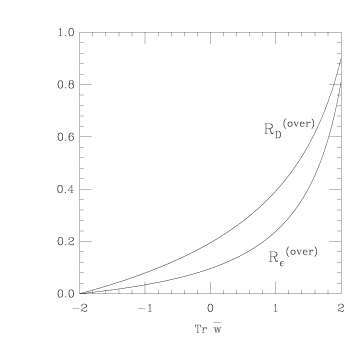
Figure 1:  Plot of the ratios $\,{\cal R}^{(over)}_{{\cal E}}(\mbox{\boldmath$y$})\,$ and $\,{\cal R}^{(over)}_{{\cal D}}(\mbox{\boldmath$y$})\,$ as functions of $\,\mbox{Tr}\,{\widetilde{w}}={\cal T}\,$, for comparison between the overrelaxation method at $\,\omega=1.9\,$ and the Los Alamos method.

3.4 Stochastic Overrelaxation Method

The stochastic overrelaxation method [13] is also a local algorithm. In this case, instead of always applying the descent step $g(\mbox{\boldmath$y$})\rightarrow g^{(LosAl.)}(\mbox{\boldmath$y$})$ one uses the new update

$$g(\mbox{\boldmath$y$})\,\rightarrow\,g^{(new)}(\mbox{\boldmath$y$})\,=\,g^{(stoc)}(\mbox{\boldmath$y$})\,\equiv\,\left\{\begin{array}[]{ll}\left[\,{\widetilde{w}}^{\dagger}(\mbox{\boldmath$y$})\,\right]^{2}\,g(\mbox{\boldmath$y$})&\quad\mbox{with probability $p$}\\ \phantom{}&\phantom{}\\ g^{(LosAl.)}(\mbox{\boldmath$y$})&\quad\mbox{with probability $1-p$}\end{array}\right.$$ (3.32)

with $0<p<1$. Of course for $p=0$ this algorithm coincides with the Los Alamos method while, for $p=1$, it does not converge at all since, as we saw in formula (3.21), the value of the minimizing function ${\widetilde{\cal E}}\left[g(\mbox{\boldmath$y$})\right]$ remains constant. However, for $p\in(0,\,1)$, the fact that, with probability $p$, a big move is done in the configuration space without changing the value of ${\widetilde{\cal E}}\left[g(\mbox{\boldmath$y$})\right]$ has, again, the capability of speeding up the relaxation process. To check this point we can compute the length of the move

$$g(\mbox{\boldmath$y$})\,\rightarrow\,\left[\,{\widetilde{w}}^{\dagger}(\mbox{\boldmath$y$})\,\right]^{2}\,g(\mbox{\boldmath$y$})\;\mbox{;}$$ (3.33)

by using equation (2.9) we can rewrite $\left[\,{\widetilde{w}}^{\dagger}(\mbox{\boldmath$y$})\,\right]^{2}$ as

$$\left[\,{\widetilde{w}}^{\dagger}(\mbox{\boldmath$y$})\,\right]^{2}\,=\,{\widetilde{w}}^{\dagger}(\mbox{\boldmath$y$})\,{\cal T}(\mbox{\boldmath$y$})\,-\,1\!\!\!\bot$$ (3.34)

and [see equation (2.35)] we easily obtain

$${\cal D}^{(stoc)}(\mbox{\boldmath$y$})\,=\,\sqrt{\,4\,-\,{\cal T}^{2}(\mbox{\boldmath$y$})}\,=\,\sqrt{\,2\,+\,{\cal T}(\mbox{\boldmath$y$})}\;\,{\cal D}^{(LosAl.)}(\mbox{\boldmath$y$})\;\mbox{.}$$ (3.35)

Roughly speaking, we can say that the stochastic overrelaxation method alternates updates that give the maximum negative variation of $\,{\widetilde{\cal E}}\,$ with steps that produce “very long” moves in the configuration space, without increasing the value of the minimizing function. This is similar in spirit to the idea behind the so-called hybrid version of overrelaxed algorithms [22, 25, 29], which are used to speed up Monte Carlo simulations with spin models, lattice gauge theory, etc. In these algorithms, $n$ microcanonical (or energy conserving) update sweeps are done followed by one standard local ergodic update (like Metropolis or heat-bath) sweeping over the lattice. Actually, for the gaussian model, it has been proven [25] that the best result is obtained when the $n$ microcanonical steps are picked at random, namely when $n$ is the average number of microcanonical sweeps between two subsequent ergodic updates. This is essentially what is done in the stochastic overrelaxation method, with $n/(n+1)$ equals in average to $p$ or, equivalently, $n$ equals in average to $p/(1-p)$.

Finally, formula (3.34) can also be used in order to reduce the overhead of the algorithm; we can in fact rewrite (3.32) as

$$g^{(stoc)}(\mbox{\boldmath$y$})\,=\,\left\{\begin{array}[]{ll}{\widetilde{h}}^{\dagger}(\mbox{\boldmath$y$})\,{\cal T}(\mbox{\boldmath$y$})\,-\,g(\mbox{\boldmath$y$})&\quad\mbox{with probability $p$}\\ \phantom{}&\phantom{}\\ {\widetilde{h}}^{\dagger}(\mbox{\boldmath$y$})&\quad\mbox{with probability $1-p$}\end{array}\right.$$ (3.36)

[ where $\,{\widetilde{h}}\,$ was introduced in (2.28) ], namely instead of computing matrix products of the form ${\widetilde{h}}^{\dagger}(\mbox{\boldmath$y$})\,g^{\dagger}(\mbox{\boldmath$y$})\,{\widetilde{h}}^{\dagger}(\mbox{\boldmath$y$})$ we just have to do a simple linear combination of ${\widetilde{h}}^{\dagger}(\mbox{\boldmath$y$})$ and $g(\mbox{\boldmath$y$})\,$.

3.5 Fourier Acceleration

The idea of Fourier acceleration [14] is very simple. If we consider the Cornell method, it is immediate from formula (3.8) that its convergence is controlled by the quantity $a^{2}\,g_{0}\,(\nabla\cdot A^{\left(g\right)})(\mbox{\boldmath$y$})\,$. For the abelian case in the continuum it can be shown [14], by analyzing the relaxation of the different components of this matrix in momentum space, that

$$(\nabla\cdot{\widetilde{A}}^{\left(g\right)})_{t}\,(\mbox{\boldmath$k$})\,\approx\,(\nabla\cdot{\widetilde{A}}^{\left(g\right)})_{0}\,(\mbox{\boldmath$k$})\,\exp\left(-\alpha\,p^{2}(\mbox{\boldmath$k$})\,t\,\right)\;\mbox{,}$$ (3.37)

namely each component decays as $\,\exp(-\alpha\,p^{2}(\mbox{\boldmath$k$})\,t\,)\,$, where $\,t\,$ indicates the number of sweeps. This means that their decay rates are approximatively equal to $1/(\alpha\,p^{2}(\mbox{\boldmath$k$})\,)\,$. Therefore, if we choose $\,\alpha\propto p^{-2}_{max}\,$ we obtain that the slowest mode has a relaxation time $\tau$ proportional to $p^{2}_{max}/p^{2}_{min}\,$. In a lattice with $N$ points on each side we have $p^{2}_{max}\propto{\cal O}(1)$ and $p^{2}_{min}\propto{\cal O}(N^{-2})\,$, namely

$$\tau\propto N^{2}\;\mbox{.}$$ (3.38)

From this analysis it is clear how, for the abelian case, the relaxation process can be speeded up: given the matrix $a^{2}\,g_{0}\,(\nabla\cdot A^{\left(g\right)})(\mbox{\boldmath$x$})\,$, we take its Fourier transform, we multiply each component in momentum space by $p^{2}_{max}/p^{2}(\mbox{\boldmath$k$})\,$, we evaluate the inverse Fourier transform and, finally, the result is used in equation (3.9) instead of the original matrix $a^{2}\,g_{0}\,(\nabla\cdot A^{\left(g\right)})(\mbox{\boldmath$y$})\,$. In a more concise form we can write:

$$R^{(update)}(\mbox{\boldmath$y$})\,\propto\,1\!\!\!\bot-{\widehat{F}}^{-1}\left\{\,\frac{p^{2}_{max}}{p^{2}(\mbox{\boldmath$k$})}\,{\widehat{F}}\left[\,\alpha\,a^{2}\,g_{0}\,\left(\nabla\cdot A^{\left(g\right)}\right)\right]\,\right\}(\mbox{\boldmath$y$})\;\mbox{;}$$ (3.39)

where ${\widehat{F}}$ indicates the Fourier transform and ${\widehat{F}}^{-1}$ is its inverse. In this way we should obtain that the components in momentum space of $a^{2}\,g_{0}\,(\nabla\cdot A^{\left(g\right)})(\mbox{\boldmath$y$})\,$ decay as

$$\exp\left(-\alpha\,p^{2}(\mbox{\boldmath$k$})\,t\,\frac{p^{2}_{max}}{p^{2}(\mbox{\boldmath$k$})}\right)\,=\,\exp\left(-\alpha\,p^{2}_{max}\,t\right)$$ (3.40)

which, with the choice $\alpha\propto p^{-2}_{max}\,$, gives $\tau\propto{\cal O}(1)$ for every component.

Of course, for the non-abelian case, this analysis becomes more complicated. Nevertheless, it is still believed that the Cornell method will have [8, 14] the behavior (3.38), and that the strategy to be used in the Fourier acceleration is given by the modified update (3.39). The main difficulty arises from the fact (see again [14]) that, instead of the eigenvalues of the laplacian $\partial^{2}$ (i.e. instead of $p^{2}(\mbox{\boldmath$k$})\,$), we have to consider the eigenvalues of the operator $\partial\cdot D$, where $D$ is the covariant derivative. Thus, the relaxation time $\tau$ will be proportional to the ratio of the largest over the smallest eigenvalue of $\partial\cdot D\,$ and the eigenvectors of this operator should be used to decompose the divergence of $A^{\left(g\right)}$. This is of course not easy to be implemented in a numerical simulation and, therefore, the eigenvectors of the laplacian are used also in the non-abelian case. The hope is that the non-abelian nature of the fields does not make the behavior of $\partial\cdot D\,$, in momentum space, too different from that of the laplacian. Actually this is more than just hope since, in the lattice Landau gauge, the link variables $\left\{U_{\mu}(\mbox{\boldmath$x$})\right\}$ are fixed as close as possible to the identity matrix (see [28], Appendix A) and therefore the operator $\partial\cdot D\,$ should be, in some sense, a “small modification” of the laplacian.

The practical implementation of the Fourier acceleration is also quite simple. In fact, we have to evaluate $a^{2}\,g_{0}\,(\nabla\cdot A^{\left(g\right)})(\mbox{\boldmath$x$})$ at each lattice site and then use formula (3.39) — where now ${\widehat{F}}$ has to be interpreted as a standard Fast Fourier Transform subroutine [10] — to find $R^{(update)}(\mbox{\boldmath$y$})$ at the given lattice site. Of course, to reduce the number of times the FFT is used, a checkerboard update should be employed. For our FFT subroutine we used as a basis in momentum space the functions $\,\exp(\,2\,\pi\,i\,\mbox{\boldmath$k$}\cdot\mbox{\boldmath$x$}\,)\,$, where $k$ has components $k_{\mu}$ given by

$$a\,k_{\mu}\,N_{\mu}\,=\,0\mbox{,}\,1\mbox{,}\,\ldots\mbox{,}\,N_{\mu}-1$$ (3.41)

and $\,\mu=1,\,\dots,d\,$. In this case the eigenvalues of the laplacian operator $\partial^{2}$ are given by the well-known formula

$$\mbox{\boldmath$p$}^{2}\,\equiv\,\frac{4}{a^{2}}\,\sum_{\mu=1}^{d}\,\sin^{2}\left(\,\pi\,a\,k_{\mu}\,\right)$$ (3.42)

and the largest eigenvalue $\,\mbox{\boldmath$p$}^{2}_{max}\,$ is obtained when

$$a\,k_{\mu}\,N_{\mu}\,=\,\lfloor\frac{N_{\mu}}{2}\rfloor$$ (3.43)

for all $\,\mu=1,\,\dots,d\,$.

Finally, it is important to observe that formula (3.39) is singular when $\,p^{2}(\mbox{\boldmath$k$})\,$ is zero. However, the zero-frequency mode of the divergence of $A^{\left(g\right)}$ does not contribute to the update (3.9); in fact, by using the periodicity of the lattice and formula (2.18), it is easy to check that

$$a^{2}\,g_{0}\,\sum_{\mbox{\boldmath$x$}}\,(\nabla\cdot A^{\left(g\right)})(\mbox{\boldmath$x$})\,=\,0\;\mbox{.}$$ (3.44)

Thus, in equation (3.39) when $\,p^{2}(\mbox{\boldmath$k$})\,$ is equal to zero, we can set the value of $p^{2}_{max}/p^{2}(\mbox{\boldmath$k$})\,$ to any finite value without affecting the performance of the method.

4 Critical Slowing-Down

To check the convergence of the gauge fixing [8, 14, 16, 18, 30] several quantities have been introduced:

$$e_{1}(t) \equiv {\cal E}(t-1)-{\cal E}(t)$$ (4.1)

$$e_{2}(t) \equiv \frac{a^{d+4}\,g^{2}_{0}}{V}\sum_{\mbox{\boldmath$x$}}\,\sum_{j=1}^{3}\,\Big{[}\left(\nabla\cdot A\right)(\mbox{\boldmath$x$})\Big{]}_{j}^{2}$$ (4.2)

$$e_{3}(t) \equiv \frac{a^{d}}{V}\sum_{\mbox{\boldmath$x$}}\,\frac{1}{2}\,\mbox{Tr}\,\left\{\left[\,1\!\!\!\bot-R^{(update)}(\mbox{\boldmath$x$})\,\right]\left[\,1\!\!\!\bot-R^{(update)}(\mbox{\boldmath$x$})\,\right]^{\dagger}\right\}$$ (4.3)

$$e_{4}(t) \equiv \max_{\mbox{\boldmath$x$}}\left[\,1\,-\,\frac{1}{2}\,\mbox{Tr}\,R^{(update)}(\mbox{\boldmath$x$})\right]$$ (4.4)

$$e_{5}(t) \equiv 1\,-\,\frac{a^{d}}{2\,V}\,\sum_{\mbox{\boldmath$x$}}\,\mbox{Tr}\,R^{(update)}(\mbox{\boldmath$x$})$$ (4.5)

where $t$ indicates the number of lattice sweeps and, when not indicated, the expressions on the r.h.s are evaluated after $t$ sweeps of the lattice are completed. All these quantities are expected to converge to zero exponentially and with the same rate [8] even though their sizes can differ considerably. Actually, it is easy to see that

$$e_{3}\,=\,\frac{2\,a^{d}}{V}\sum_{\mbox{\boldmath$x$}}\,\left[\,1\,-\,\frac{\mbox{Tr}\,R^{(update)}(\mbox{\boldmath$x$})}{2}\,\right]\,=\,2\,e_{5}\,\approx\,2\,e_{4}\;\mbox{.}$$ (4.6)

By using equation (3.10) we can also rewrite $e_{2}$ as

$$e_{2}\,=\,\frac{a^{d}}{V}\sum_{\mbox{\boldmath$x$}}\,{\cal N}^{2}(\mbox{\boldmath$x$})\,\,\left[\,1\,-\,\frac{{\cal T}^{2}(\mbox{\boldmath$x$})}{4}\,\right]\;\mbox{.}$$ (4.7)

We know that, if the algorithm converges, the matrix $R^{(update)}(\mbox{\boldmath$x$})$ should approach the identity matrix $1\!\!\!\bot$ as the number of iteration increases or, equivalently, that its trace should be very close to two at large $\,t\,$. This implies [ see the expressions of $\,R^{(update)}(\mbox{\boldmath$x$})\,$ for the various local methods: formulae (3.4), (3.13), (3.25) and (3.32) ] that $\,{\widetilde{w}}^{\dagger}(\mbox{\boldmath$x$})\to 1\!\!\!\bot\,$, and therefore ${\cal T}(\mbox{\boldmath$x$})$ is also very close to two. Therefore if $e_{4}$ is of order $\epsilon\ll 1$ then also $e_{3}\,$, $e_{5}$ and $e_{2}$ should be of this order; taking into account these relations, we decided to look only at the quantities $e_{1}$, $e_{2}$ and $e_{4}\,$.

We also expect that the spatial fluctuations of the quantities $Q_{\nu}(x_{\nu})$, defined in (2.21), and of the longitudinal gluon propagators, defined in (2.22), go to zero exponentially. Indeed, the fact that $Q_{\nu}(x_{\nu})$ should be constant is being increasingly used as a check of the accuracy of the gauge fixing [23, 31]. To check this more precisely, we introduced a new quantity defined as

$$e_{6}(t)\,\equiv\,\frac{1}{d}\,\sum_{\nu=1}^{d}\,\frac{1}{3\,N_{\nu}}\sum_{j=1}^{3}\,\sum_{x_{\nu}=1}^{N_{\nu}}\,\frac{\left[\,Q_{\nu}(x_{\nu})-{\widehat{Q}}_{\nu}\,\right]_{j}^{2}}{\left[{\widehat{Q}}_{\nu}\right]_{j}^{2}}$$ (4.8)

where

$${\widehat{Q}}_{\nu}\,\equiv\,\frac{1}{N_{\nu}}\,\sum_{x_{\nu}=1}^{N_{\nu}}\,Q_{\nu}(x_{\nu})\;\mbox{.}$$ (4.9)

For each of these quantities, in the limit of large $\,t\,$, we can introduce [3] a relaxation time $\tau_{i}$ by the relation

$$e_{i}(t)\,\approx\,c_{i}\,\exp\left(\,-\,t/\tau_{i}\,\right)\;\mbox{,}$$ (4.10)

namely

$$\tau_{i}\,\equiv\,\lim_{t\to\infty}\,\frac{-\,1}{\ln\left[\,e_{i}(t+1)/e_{i}(t)\,\right]}\;\mbox{.}$$ (4.11)

As said before, we expect all these relaxation times to coincide and be equal to $\tau$.

To analyze the critical-slowing down of an algorithm we have to measure $\,\tau\,$ for different pairs of $\,N\,$ and $\,\beta=4/g_{0}^{2}\,$, but at “constant physics”. This means that we have to keep the ratio $\,N/\xi\,$ constant, where the correlation length $\,\xi\,$ is given by the inverse of the square root of the string tension $\,\kappa\,$, i.e. $\,\xi=1/\sqrt{\kappa}\,$. The string tension for two-dimensional $SU(2)$ lattice gauge theory (in the spin-${{1\over 2}}$ representation) is given, in the infinite volume limit, by [32]

$$\kappa\,=\,-\log\frac{I_{2}(\beta)}{I_{1}(\beta)}\;\mbox{,}$$ (4.12)

where $\,I_{n}\,$ is the modified Bessel function. Thus we have

$$\xi\,=\,\frac{1}{\sqrt{-\log\frac{I_{2}(\beta)}{I_{1}(\beta)}}}$$ (4.13)

which, in the limit of large $\beta\,$, gives

$$\xi\,=\,\sqrt{\frac{2\,\beta}{3}}\,\left[\,1\,+\,\frac{1}{4\,\beta}\,+\,{\cal O}(\beta^{-2})\,\right]\;\mbox{.}$$ (4.14)

Therefore a constant ratio $\,N/\xi\,$ is equivalent, in this limit, to keeping the ratio $\,N^{2}/\beta\,$ fixed. The values for the pairs $(N,\beta)$ have been chosen in such a way that $\,N\gg\xi\,$; thus the finite size effects should be negligible. All the pairs $(N,\beta)$ used are reported in Table 1. In the same table we report the value of the corresponding correlation length $\,\xi\,$ obtained by using equation (4.13). We have chosen $\,N^{2}/\beta\,=\,32\,$ and $\,N/\xi\,\approx\,7$.

Once all these values of $\tau$ are obtained, we can try a fit of the form

$$\tau\,=\,c\,N^{z}$$ (4.15)

and find the dynamic critical exponent $z$ for that algorithm. It is important to recall that the value of $z$ obtained in this way is independent of the “constant physics” chosen ($N^{2}/\beta=32$ in our case). On the contrary, this is not the case for the constant $\,c$. In particular we expect the relaxation time $\tau$, and therefore $\,c$, to increase as the link couplings $\,U_{\mu}(\mbox{\boldmath$x$})\,$ in (2.24) become more “random”, i.e as $\beta$ decreases for a given lattice size $N$ (and the value of the ratio $N^{2}/\beta$ increases).

$N$	$8$	$12$	$16$	$20$	$24$	$28$	$32$	$36$	$64$
$\beta$	$2.0$	$4.5$	$8.0$	$12.5$	$18.0$	$24.5$	$32.0$	$40.5$	$128.0$
$\xi$	$1.09$	$1.65$	$2.24$	$2.83$	$3.42$	$4.00$	$4.58$	$5.16$	$9.22$

Table 1:  The pairs $(N,\beta)$ used for the simulations and the correlation length $\xi$ evaluated in the infinite volume limit.

5 Tuning of the Algorithms

algorithm	$a(\mbox{\boldmath$y$})$	$b(\mbox{\boldmath$y$})$
Los Alamos	$1$	$0$
Cornell	$\alpha\,{\cal N}(\mbox{\boldmath$y$})$	$\alpha\,{\cal N}(\mbox{\boldmath$y$})\,{\cal T}(\mbox{\boldmath$y$})/2\,-\,1$
overrelaxation	$\omega$	$\omega-1$
stochastic overr.	$\begin{array}[]{ll}{\cal T}(\mbox{\boldmath$y$})&\quad\mbox{with probability $p$}\\ 1&\quad\mbox{with probability $1-p$}\end{array}$	$\begin{array}[]{ll}1&\quad\mbox{with probability $p$}\\ 0&\quad\mbox{with probability $1-p$}\end{array}$

Table 2:  The coefficients $a(\mbox{\boldmath$y$})$ and $b(\mbox{\boldmath$y$})$ for the four local algorithms considered in this paper.

The implementation of all the algorithms considered in this work — except for the Los Alamos method — requires the tuning of a parameter: $\alpha$ for the Cornell method and the Fourier acceleration, $\omega$ for the overrelaxation method and $p$ for the stochastic overrelaxation. This is, of course, a potential disadvantage of all these methods and makes the study of their critical slowing-down more difficult: in fact, for each pair $(N,\beta)\,$, the value of the parameters should be tuned in such a way that the value of $\tau$ is minimized. This is usually done heuristically since, as explained in the Introduction, no rigorous analyses are available for these algorithms. However, analytic estimates for the optimal choice of $\omega$ are indeed known for the overrelaxation method applied to other numerical problems [9, 10, 11, 24, 33]; in all these cases, in the limit of large lattice size $N$, it has been found that

$$\omega_{opt}\,=\,\frac{2}{1\,+\,C_{opt}/N}$$ (5.1)

where the constant $C_{opt}$ is problem dependent. This result is usually adopted as a guess [16, 19] also for the optimal choice of $\omega$ when the overrelaxation method is applied to Landau gauge fixing.

In order to obtain simple formulae like (5.1) for the optimal choice of $\alpha$ (in the case of the Cornell method) and $p$, we decided to compare the four local algorithms considered in this work. It is interesting to notice that they can all be defined by the update

$$g(\mbox{\boldmath$y$})\,\rightarrow\,g^{(new)}\,\propto\,a(\mbox{\boldmath$y$})\,{\widetilde{h}}^{\dagger}(\mbox{\boldmath$y$})\,-\,b(\mbox{\boldmath$y$})\,g(\mbox{\boldmath$y$})$$ (5.2)

where the coefficients $a(\mbox{\boldmath$y$})$ and $b(\mbox{\boldmath$y$})$ are given in Table 2. Moreover, we see from our simulations that in all methods, usually after a few sweeps, we have ${\cal T}(\mbox{\boldmath$y$})\mathrel{\hbox to0.0pt{\lower 3.0pt\hbox{$\mathchar 536\relax$}\hss}\raise 2.0pt\hbox{$\mathchar 316\relax$}}2\,$. This is evident by looking at the decay of $\,e_{2}(t)\,$ (see Figures 2 and 3 for typical examples) and considering formula (4.7). Actually, since the gauge-fixing procedure is stopped when $\,e_{2}(t)\,$ is smaller than $10^{-12}$ (see end of Section 6), the condition $\,{\cal T}\mathrel{\hbox to0.0pt{\lower 3.0pt\hbox{$\mathchar 536\relax$}\hss}\raise 2.0pt\hbox{$\mathchar 316\relax$}}2\,$ is satisfyed for the most part of our simulations. With this in mind we can write

$$g(\mbox{\boldmath$y$})\,\rightarrow\,g^{(new)}\,\approx\,{\tilde{a}}(\mbox{\boldmath$y$})\,{\widetilde{h}}^{\dagger}(\mbox{\boldmath$y$})\,-\,{\tilde{b}}(\mbox{\boldmath$y$})\,g(\mbox{\boldmath$y$})$$ (5.3)

where the coefficients ${\tilde{a}}(\mbox{\boldmath$y$})$ and ${\tilde{b}}(\mbox{\boldmath$y$})$ are obtained from the coefficients $a(\mbox{\boldmath$y$})$ and $b(\mbox{\boldmath$y$})$ by imposing the condition ${\cal T}(\mbox{\boldmath$y$})=2$.

This simple analysis seems to suggest (see Table 2) that the Cornell method is equivalent to the overrelaxation method if we make the substitution

$$\alpha\,{\cal N}(\mbox{\boldmath$y$})\,\rightarrow\,\omega\;\mbox{.}$$ (5.4)

The same substitution is suggested by considering the ratios ${\cal R}_{{\cal E}}(\mbox{\boldmath$y$})$ and ${\cal R}_{{\cal D}}(\mbox{\boldmath$y$})$ defined in (3.1) and (3.2); in fact, as ${\cal T}(\mbox{\boldmath$y$})$ goes to $2$, we have that the formulae for these ratios for the Cornell method and for the overrelaxation method coincide if the above substitution is employed (see end of Sections 3.2 and 3.3 respectively).

If this analysis is correct we should obtain for the Cornell method the same dynamic critical exponent as for the overrelaxation method, i.e. $\,z\approx 1\,$. This will be verified in Section 7. As a further check of this “equivalence” between the two methods we can compare the optimal choices for their tuning parameters, obtained in our simulations. We notice that while $\,\omega\,$ and $\,\alpha\,$ are fixed parameters throughout the run, $\,{\cal N}(\mbox{\boldmath$y$})\,$ changes with the iterations, and we are interested in its value as $\,{\cal T}(\mbox{\boldmath$y$})\to 2\,$. Moreover, $\,{\cal N}(\mbox{\boldmath$y$})\,$ is a local quantity, and therefore we consider its space average, which can be easily estimated in this limit. In order to do this, let us rewrite the minimizing function as

$${\cal E} = 1-\frac{a^{d}}{4\,d\,V}\sum_{\mu=1}^{d}\sum_{\mbox{\boldmath$x$}}\,\mbox{Tr}\;\left\{\,U_{\mu}^{\left(g\right)}(\mbox{\boldmath$x$})\,+\,\left[U_{\mu}^{\left(g\right)}(\mbox{\boldmath$x$}-a\mbox{\boldmath$e$}_{\mu})\right]^{\dagger}\,\right\}$$ (5.5)

$$= 1-\,\frac{a^{d}}{4\,d\,V}\sum_{\mbox{\boldmath$x$}}\,\mbox{Tr}\,w(\mbox{\boldmath$x$})\,=\,\,\frac{a^{d}}{4\,d\,V}\sum_{\mbox{\boldmath$x$}}\,{\cal N}(\mbox{\boldmath$x$})\,{\cal T}(\mbox{\boldmath$x$})$$

which, in the limit ${\cal T}(\mbox{\boldmath$y$})\rightarrow 2$, gives

$${\cal E}\,=\,1-\,\frac{a^{d}}{2\,d\,V}\sum_{\mbox{\boldmath$x$}}\,{\cal N}(\mbox{\boldmath$x$})\;\mbox{.}$$ (5.6)

In other words, the space average of $\,{\cal N}(\mbox{\boldmath$x$})\,$ is given by

$$2\,d\,\left(\,1-{\cal E}_{stat}\,\right)\;\mbox{,}$$ (5.7)

where $\,{\cal E}_{stat}\,$ is the value of the minimizing function at the stationary point. Of course this value is not known a priori but, for fixed values of $\beta$ and $V$, its order of magnitude can be easily estimated with just a few numerical tests. Using this result, we are able to make a numerical comparison between the tuning parameters for the two methods (see Section 7), finding very good agreement.

One may also attempt to establish a relation between the overrelaxation and the stochastic overrelaxation. For example, we can try to write the update (3.32) as an average of the two cases with weights $p$ and $1-p$ obtaining (in the limit ${\cal T}(\mbox{\boldmath$y$})\rightarrow 2$)

$$g^{(stoc)}(\mbox{\boldmath$y$})\,\approx\,\left(\,1+p\right)\,{\widetilde{h}}^{\dagger}(\mbox{\boldmath$y$})\,-\,p\,g(\mbox{\boldmath$y$})\;\mbox{,}$$ (5.8)

which suggests the substitution

$$p\,\rightarrow\,\left(\,\omega\,-\,1\,\right)\;\mbox{.}$$ (5.9)

However, if we now look at the ratios ${\cal R}_{{\cal E}}(\mbox{\boldmath$y$})$ and ${\cal R}_{{\cal D}}(\mbox{\boldmath$y$})$ for the update (5.8) we obtain, as ${\cal T}(\mbox{\boldmath$y$})$ goes to $2$,

$${\cal R}^{(stoc)}_{{\cal E}}(\mbox{\boldmath$y$})\,\rightarrow\,p$$ (5.10)

and

$${\cal R}^{(stoc)}_{{\cal D}}(\mbox{\boldmath$y$})\,\rightarrow\,p\;\mbox{;}$$ (5.11)

the second formula, if compared to (3.31), seems to be consistent with the substitution (5.9) while the first [compared to (3.30)] suggests the relation

$$p\,\rightarrow\,\left(\,\omega\,-\,1\,\right)^{2}\;\mbox{.}$$ (5.12)

These two possibilities will be tested numerically (see Section 7) by plotting the quantities $\,(\,\omega\,-\,1\,)\,/\,p\,$ and $\,(\,\omega\,-\,1\,)^{2}/\,p\,$ as a function of $\,N$.

Finally, we do not hazard here any hypothesis on the tuning of $\,\alpha\,$ for the Fourier acceleration method.

6 Numerical Simulations

To thermalize the gauge configuration $\{U_{\mu}(\mbox{\boldmath$x$})\}$ at a fixed value of the coupling $\beta\,$, we used a standard heat-bath algorithm [34]. In order to optimize the efficiency of the code, we used two different $SU(2)$ generators (methods 1 and 2 described in Appendix A in [35], with $h_{cutoff}=2$).

With the pairs $(N,\beta)$ that we considered (see Section 4), we should always have $\,N\gg\xi\,$ and therefore we expect all the temporal correlations to decay exponentially. As a check we measured, for all the pairs $(N,\beta)$, the integrated autocorrelation time for the Wilson loop $\,W(1,1)\,$ and for the Polyakov loop $P\,$ (indicated respectively as $\,\tau_{int,W_{1}}\,$ and $\,\tau_{int,P}\,$). Moreover, for the pairs $(N,\beta)$ used for the Fourier acceleration method, we also measured the integrated autocorrelation time $\,\tau_{int,W_{l}}\,$ for the Wilson loops $\,W(l,l)\,$ with $\,l\,=\,2\mbox{,}\,4\mbox{,}\,8\mbox{,}\,\ldots\mbox{,}\,N/2\,$.

In practice, we started all our runs with a random $\{U_{\mu}(\mbox{\boldmath$x$})\}$ configuration and we did $\,5000\,$ sweeps for thermalization. The configurations used for gauge fixing were separated by $\,100\,$ sweeps, in order to get a statistically independent sample. After discarding $\,4900\,$ sweeps out of a total of 54900 sweeps, we evaluated $\,\tau_{int,W_{l}}\,$ and $\,\tau_{int,P}\,$ by using a window of $\,4\,\tau_{int}\,$, which is a reasonable choice if the decay is roughly exponential. For the observables we considered we obtained $\,0.5\mathrel{\hbox to0.0pt{\lower 3.0pt\hbox{$\mathchar 536\relax$}\hss}\raise 2.0pt\hbox{$\mathchar 316\relax$}}\tau_{int}\mathrel{\hbox to0.0pt{\lower 3.0pt\hbox{$\mathchar 536\relax$}\hss}\raise 2.0pt\hbox{$\mathchar 316\relax$}}10\,$. Noticing that $\tau_{int}=0.5\,$ indicates that the data are uncorrelated, we can conclude, as expected, that the system decorrelates rather fast and that the configurations used for testing the gauge-fixing algorithms are essentially statistically independent.

The tuning of the parameters $\omega$, $p$ and $\alpha\,$ — respectively for the overrelaxation, the stochastic overrelaxation, the Cornell and the Fourier acceleration methods — was done very carefully. More precisely, we divided it in three parts. In the first step, we considered a few values of the parameter spread in a large interval. For example we used $\omega=1.1\mbox{,}\,1.2\mbox{,}\,\ldots\mbox{,}\,1.9$ or $p=0.1\mbox{,}\,0.2\mbox{,}\,\ldots\mbox{,}\,0.9\,$. For each of these values we gauge fixed $10$ different configurations, measured all the $\,\tau_{i}\,$’s and averaged the results. In this way we were able to select a smaller interval for the parameter (usually of length $\approx 0.2$ for the overrelaxation or the stochastic overrelaxation methods) which was used in the second step of the tuning. In this case $20$ configurations were analyzed for each value of the parameter (and these values were typically separated by $0.01\,$ for the overrelaxation and stochastic overrelaxation methods). In the last step, the length of the interval was further reduced and $100$ configurations were gauge-fixed for each value of the parameter.

A total of $\,201.7\,$ hours of CPU were used for the four methods requiring tuning. Of these, $\,21.6\,$ were used for the first level of tuning, $\,36.1\,$ for the second level and the remaining $\,144\,$ for the third level.

For the Los Alamos method no tuning is needed, but we found that, in this case, the fluctuations for the relaxation times are larger and therefore more configurations ($500\,$, to be exact) had to be considered, for a total of $\,23.3\,$ hours of CPU.

Finally, for measuring the relaxation time $\,\tau_{i}\,$ (with $\,i\,=\,1\mbox{,}\,2\mbox{,}\,4\,$ and $6$) we did a chi-squared fitting of the functions $\,\log e_{i}(t)\,$ which, if relation (4.10) is satisfied, should be a straight line. Indeed this was usually the case already after a few initial sweeps of the lattice, at least for the quantities $\,e_{1}\,$, $\,e_{2}\,$ and $\,e_{4}\,$. On the contrary, the decay of $\,e_{6}\,$ is really smooth and monotonic only for the Fourier acceleration method. As an example we show, in Figure 2, the behavior of $\,e_{2}\,$ and $\,e_{6}\,$ as functions of $\,t\,$ for the Cornell and the Fourier acceleration method. We also show, in Figure 3, the decays of the four quantities for the stochastic overrelaxation method.

We use the condition

$$e_{2}\,\leq\,10^{-12}$$ (6.1)

to stop the gauge fixing, in order to ensure that enough data are produced for the fitting and that, when the procedure is stopped, essentially only the slowest mode has survived. To get rid of the initial fluctuations, we used only the last $100$ data when the total number of sweeps $N_{sw}$ was larger than $200\,$, or the second half of the data when less than $200\,$ sweeps were necessary to fix the gauge. For $\,i\,=\,1\,$ we have also to take into account possible fluctuations of $\,e_{1}(t)\,$ around zero, which appear when the minimizing function is fixed within the machine precision. Therefore, for this quantity, we also discarded the last $50$ sweeps, if $N_{sw}>200$, or the last one quarter of the data if $N_{sw}$ was smaller than $200$.

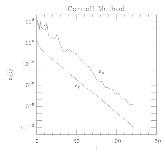
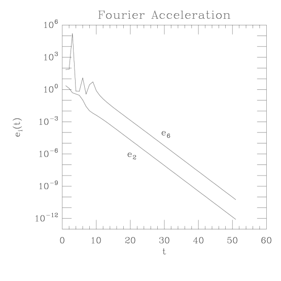
Figure 2:  Plot of the decays of the quantities $\,e_{2}\,$ and $\,e_{6}\,$ as functions of $\,t\,$ for (a) the Cornell method, with $\alpha=0.481$, and (b) the Fourier acceleration method, with $\alpha=0.160$. Both plots were done for $\,16^{2}\,$ lattices.

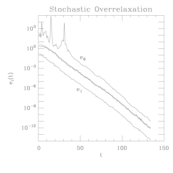
Figure 3:  Plot of the decays of the quantities $\,e_{1}\,$, $\,e_{2}\,$, $\,e_{4}\,$ and $\,e_{6}\,$ as functions of $\,t\,$ for the stochastic overrelaxation method, with $p=0.75$ on a $\,16^{2}\,$ lattice. The two almost superposed curves are $\,e_{2}(t)\,$ and $\,e_{4}(t)\,$ ($\,e_{2}(t)\,$ is the “smoother” curve).

7 Results and Conclusions

Our final data for the relaxation times are reported, for the different methods, in Tables 5–9. We show for each algorithm only the relaxation time $\,\tau_{2}\,$ for the quantity $\,e_{2}\,$ defined in (4.2). Indeed, we checked that, for all methods and pairs $\,(N,\beta)\,$, the four measured relaxation times were in agreement within error bars. We also show the optimal choice for the tuning parameter (when needed), the number of sweeps necessary to reach the stopping condition (6.1), and, for the Cornell method, the value of the minimizing function (used in Section 7.3 for comparison with the overrelaxation method). Averages are taken over the different configurations that were gauge fixed for each pair $\,(N,\beta)\,$.

7.1 Critical Exponents

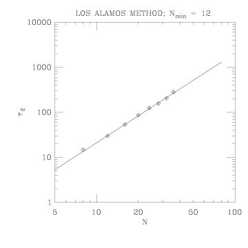
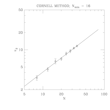
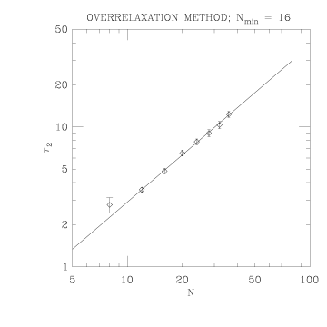
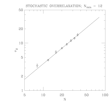
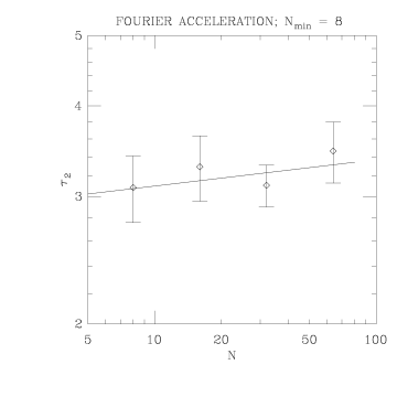
Figure 10:  Power-law fit for (a) the Los Alamos method, (b) the Cornell method, (c) the overrelaxation method, (d) the stochastic overrelaxation method and (e) the Fourier acceleration method.

We now proceed to the evaluation of the dynamic critical exponents $\,z\,$. In Tables 10–14 we present the results of the fits to the ansatz (4.15) for $\,\tau_{2}\,$ for the various methods. We do a weighted least-squares fit in several “steps”, discarding at each step the values of $\,N\,$ smaller than $\,N_{min}\,$. In this way we try to rule out some of the smaller values of $\,N\,$ as finite-size corrections; this is very important since we are dealing with very small lattice sizes. We do so for all possible values of $\,N_{min}\,$, and decide which one gives the best fit for $z$ by comparing $\,\chi^{2}\,$ and confidence levels for the different $\,N_{min}\,$’s. As can be seen from our tables, these finite-size corrections are negligible already at lattice sizes $12$ or $16$. In Figure 10 we plot together the values of $\,\tau_{2}\,$ and the fitting curve for our preferred fit for the various algorithms.

Our results for the dynamic critical exponents are in agreement with what is generally expected, namely we find: $\,z\approx\,2\,$ for the Los Alamos method, $\,z\approx\,1\,$ for the overrelaxation [19] and the stochastic overrelaxation method, and $\,z\approx\,0\,$ for the Fourier acceleration method. For the Cornell method, as mentioned in Section 3.5, a simple analysis (based on the abelian case in the continuum) would give $\,z\approx 2\,$, and this is what is generally believed [8, 14]. On the other hand, our comparative analysis between the Cornell and the overrelaxation methods in Section 5 would suggest $\,z\approx 1\,$. As can be seen from Table 11, our results show the latter behavior. Furthermore, in Section 7.3 we will verify the relation between the tuning parameters for these two methods found in Section 5.

Actually, the dynamic critical exponent $\,z\,$ for the Cornell method is even slightly smaller than one. The good performance of this method could be understood by noticing that the value of $\alpha\,{\cal N}(\mbox{\boldmath$x$})$ changes during the gauge-fixing process. In particular, with a few numerical tests, it can be checked that the space average value of ${\cal N}(\mbox{\boldmath$x$})$ increases with the iterations. Moreover, as we will see below, the final value of $\alpha\,{\cal N}(\mbox{\boldmath$x$})$ is equal to the optimal value found for $\omega$ in the overrelaxation method. So, in a sense, we have an overrelaxation method whose parameter $\omega\leftrightarrow\alpha\,{\cal N}(\mbox{\boldmath$x$})$ increases with the iterations from an initial value $\omega_{0}$ up to the asymptotic value $\omega_{opt}\,$. It is well known [10, 22] that in overrelaxed algorithms the optimal strategy is precisely to vary the parameter $\omega$ from an initial value $1$ to a larger asymptotic value $\omega_{opt}\,$, which is usually done by using Chebyshev polynomials. It is conceivable that the Cornell method does this variation “automatically” and this could explain why it performs slightly better than the overrelaxation method.

7.2 Checking the gauge fixing

For each gauge-fixed configuration we also measured the ratios

$$r_{i}\,\equiv\,\frac{e_{i}}{e_{2}}$$ (7.1)

with $\,i=1\mbox{,}\,4\,$ and $6\,$. For the cases $\,i=1\,$ and $\,i=4\,$ this quantity is essentially independent of the configuration and of the lattice size; therefore, for each algorithm, after averaging over all the configurations, we take a final average over all the pairs $(N,\beta)\,$. The results are given in Table 3. From that it is clear that the quantities $\,e_{1}\,$, $\,e_{2}\,$ and $\,e_{4}$ not only decay with the same rate (as said above) but also have the same order of magnitude.

The situation for the ratio $\,e_{6}\,$ is considerably more complicated. In fact, its value depends strongly not only on the algorithm and on the lattice size $\,N\,$ but also on the underlying configuration $\left\{U_{\mu}(\mbox{\boldmath$x$})\right\}$. Namely, this quantity fluctuates so much that if the average is taken over all the gauge-fixed configurations, at a fixed lattice size, the corresponding standard deviation is often comparable in magnitude to the average itself. As an example, see Table 4 where we show our results for all the methods on a $32^{2}\,$ lattice. From these data (see also Figures 2 and 3) it is clear that the Fourier acceleration method achieves a much faster decay for $\,e_{6}\,$ than the Los Alamos method, the Cornell method and the overrelaxation method. Actually this was expected. In fact, by using one of these three local methods it can be easily checked that, even when the condition (6.1) is satisfied, the quantities $\,Q_{\nu}\,$ [defined in (2.21)] are usually not constant but show a kind of long-wavelength spatial fluctuation. The Fourier acceleration method treats all the wavelength in the same way and therefore it is not surprising that it is very effective in reducing these spatial fluctuations. More surprising is the good performance of the stochastic relaxation method which, although a local method, also appears to be very efficient in reducing the fluctuations of $\,Q_{\nu}\,$. Why this happens is not clear to us.

algorithm	$r_{1}$	$r_{4}$
Los Alamos	$0.2445\pm 0.0008$	$0.5197\pm 0.0113$
Cornell	$0.1490\pm 0.0054$	$4.5212\pm 0.5858$
overrelaxation	$0.1061\pm 0.0106$	$3.2357\pm 0.3482$
stochastic overr.	$0.0151\pm 0.0039$	$0.9642\pm 0.0214$
Fourier acceleration	$0.0483\pm 0.0148$	$1.0219\pm 0.0374$

Table 3:  The ratios $\,r_{1}\,$ and $\,r_{4}\,$ for each algorithm. Averages are taken first over the gauge-fixed configurations and then over the different pairs $(N,\beta)\,$. The error bars are one standard deviation.

algorithm	$r_{6}$	$\min r_{6}$	$\max r_{6}$
Los Alamos	$10.7\times 10^{6}\pm 4.9\times 10^{6}$	$4939.7$	$2.23\times 10^{9}$
Cornell	$19.3\times 10^{6}\pm 19.0\times 10^{6}$	$86.3$	$1.90\times 10^{9}$
overrelaxation	$2.4\times 10^{5}\pm 1.2\times 10^{5}$	$34.1$	$1.1\times 10^{7}$
stochastic overr.	$3.9\times 10^{3}\pm 2.0\times 10^{3}$	$4.93$	$1.8\times 10^{5}$
Fourier acceleration	$5.6\times 10^{3}\pm 4.5\times 10^{3}$	$0.84$	$4.5\times 10^{5}$

Table 4:  The ratio $\,r_{6}\,$ (average, minimum and maximum value) for each algorithm. Averages are taken over the gauge-fixed configurations for $N=32\,$ (for other lattice sizes the results are similar). The error bars are one standard deviation.

7.3 Discussion of the Tuning of the Algorithms

Let us now discuss the tuning of the different methods. The values for the optimal choice of the various parameters, for different pairs $(N,\beta)\,$, are reported in Tables 6–9. An estimate of their uncertainties is also indicated. From our simulations we noticed that a good tuning becomes more and more important as the lattice size increases. At small lattice sizes, in fact, the relaxation time $\tau$ displays a kind of plateau around the minimum while, as $N$ increases, the absolute minimum becomes more and more pronounced. The uncertainties indicated in these tables are therefore slightly under-estimated for the smaller lattice sizes, and slightly over-estimated for the larger lattice sizes. In Figure 4, as an example, we show typical graphs of our tuning parameters for some of the larger values of $N\,$, done at the “third level” of tuning (see Section 6).

We now try to verify, using our data, the expressions suggested in Section 5 for the various tuning parameters.

In order to check the relation (5.1) for the optimal choice of the overrelaxation parameter $\omega\,$, we rewrote that equation as

$$\frac{2\,-\,\omega_{opt}}{\omega_{opt}}\,=\,\frac{C_{opt}}{N}$$ (7.2)

and fitted our results to find a value for the constant $C_{opt}\,$. After discarding the datum for $N=8$, we obtained $C_{opt}\,=\,1.53\pm 0.35\,$. In Figure 5 we show, together, the data and the fitting curve.

For the parameter $\alpha$ of the Cornell method we do not have a simple formula as (7.2) but we have conjectured, in Section 5, a relation between $\omega_{opt}$ and $\alpha_{opt}$. Namely we suggested [see formulae (5.4) and (5.7)]

$$\omega_{opt}\,=\,\alpha_{opt}\,2\,d\,\left(\,1\,-\,{\cal E}_{stat}\,\right)\;\mbox{,}$$ (7.3)

where $d$ is the dimension of the lattice and ${\cal E}_{stat}$ is the value of the minimizing function at the minimum. By using the data reported in Tables 6 and 7 we plotted together, in Figure 6, both sides of this equation. The agreement is clearly good.

Finally we checked the two relations introduced in Section 5 between $\omega$ and the tuning parameter $p$ for the stochastic overrelaxation method. In particular we plotted, in Figure 7, the two ratios

$$\frac{\omega_{opt}\,-\,1}{p_{opt}}\qquad\mbox{and}\qquad\frac{\left(\,\omega_{opt}\,-\,1\,\right)^{2}}{p_{opt}}$$ (7.4)

as a function of $\,N\,$. If one of these relations [ see formulae (5.9) and (5.12) ] is correct we should obtain, for the corresponding ratio, a constant value $1$. From our data it is not possible to reach a definite conclusion, but the first hypothesis, namely

$$\frac{\omega_{opt}\,-\,1}{p_{opt}}\;=\;1\;\mbox{,}$$ (7.5)

seems to be slightly better verified.

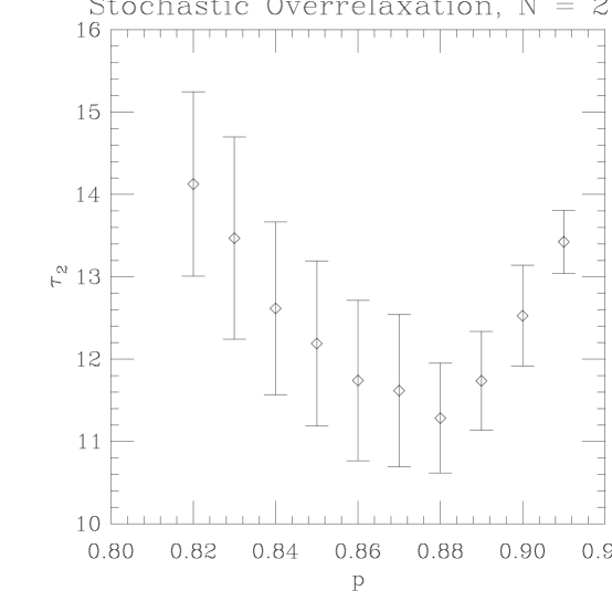
Figure 4:  Plot of the third level of tuning respectively for (a) the overrelaxation method, at lattice size 20, and (b) the stochastic overrelaxation method, at lattice size 28. Error bars are one standard deviation. Note that points are correlated, since the same 100 configurations are used for each value of the tuning parameter.

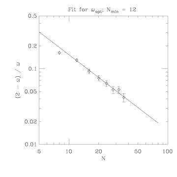
Figure 5:  Plot of the ratio $\,(2-\omega_{opt})/\omega_{opt}\,$ (symbol: $\diamond$) as a function of $N\,$. The solid line is the fitting curve $\,C_{opt}/N\,$ with $\,C_{opt}=1.53$.

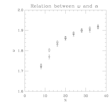
Figure 6:  Plot of $\,\omega_{opt}\,$ (symbol: $\diamond$) and $\,\alpha_{opt}\,{\cal N}$ (symbol: $\Box$) as a function of $N$ with $\,{\cal N}\,$ given by equation (5.7).

Figure 7:  Plot of $\,(\omega_{opt}-1)/p_{opt}\,$ (symbol: $\diamond$) and $\,(\omega_{opt}-1)^{2}/p_{opt}$ (symbol: $\Box$) as a function of $N$. In order to check the two hypotheses introduced in Section 5, the constant curve $1$ is also shown.

7.4 Computational Cost of the Algorithms

To check the computational cost of the algorithms we estimated the CPU time $T_{gf}$ necessary to update a single site variable $g(\mbox{\boldmath$x$})$ by using the fortran function mclock. As expected, the four local methods have very similar values for $T_{gf}\,$ and essentially independent of the volume. In particular we found $T_{gf}\approx 9\mu s$ for the Los Alamos method, $T_{gf}\approx 9.5\mu s$ for the Cornell method, $T_{gf}\approx 11.5\mu s$ for the overrelaxation method and $T_{gf}\approx 10.5\mu s$ for the stochastic overrelaxation method.

For the case of the Fourier acceleration method $T_{gf}$ should increase [10] as $\log N\,$. We did a least-squares fit of our data to the ansatz

$$T_{gf}\,=\,A\,\log N\,+\,B$$ (7.6)

and we obtained $\,A\,=\,48.91\,\pm\,0.11\,$ and $\,B\,=\,-54.42\,\pm\,0.45\,$, both measured in microseconds. In Figure 8 we show the points and the fitting curve. For our range of lattice sizes, $\,T_{gf}\,$ for the Fourier acceleration varied from $56\,\mu s$ to $148\,\mu s\,$. Of course, this “loss” in efficiency, with respect to the local algorithms, has to be taken into account when the computational cost of this algorithm is analyzed. In fact, even though the Fourier acceleration method succeeds in eliminating critical slowing-down, and therefore is more advantageous than the improved local method in terms of the number of sweeps $N_{sw}\,$ required to achieve gauge fixing, its performance is effectively better only at very large lattices.

To illustrate this, let us compare the true CPU time needed to gauge fix a configuration using Fourier acceleration and our best improved local algorithm: the Cornell method. Since we want to evaluate the total CPU time we have to look at the number of sweeps $N_{sw}\,$, needed in average to achieve gauge fixing, as a function of $N$. This quantity behaves in a manner similar to the relaxation time $\tau\,$, namely it diverges with $N$ as a power of some dynamic critical exponent $\,z_{nsw}\,$. This exponent should be similar to, but strictly smaller than the exponent $z$ for the relaxation times. In fact, $\,N_{sw}\,$ is a quantity involving the behavior of the whole gauge-fixing process, and therefore it includes faster modes (modes with “smaller exponents”) for the first few iterations, while the relaxation time $\,\tau\,$ is evaluated in the limit of large $t$, i.e. when essentially only the slowest mode has survived. The exponents $\,z_{nsw}\,$ for the various methods can be obtained, together with the respective proportionality constants $\,c_{nsw}\,$, from a fitting of the data in Tables 5–9, analogously to what was done for the $z$’s. For the Cornell method we obtain $\,z_{nsw}\approx 0.77\,$ (which should be compared to $\,z\approx 0.82\,$ for the relaxation time) and $c_{nsw}\approx 18\,$, while for the Fourier acceleration we get $\,z_{nsw}\approx 0$ (as expected) and $c_{nsw}\approx 67\,$. From these estimates, the value $T_{gf}\approx 9.5\mu s$ for the Cornell method and the fit (7.6) for the Fourier acceleration method, we can get the following approximate expressions for the time, in microseconds, necessary to gauge fix a configuration:

$$CPUtime\;\approx\;\left\{\begin{array}[]{ll}9.5\,\left(\,18\,N^{0.77}\,\right)\,N^{2}\,\mu s&\quad\mbox{Cornell method}\\ \phantom{}&\phantom{}\\ \left(\,49\log N\,-\,54\,\right)\,67\,N^{2}\,\mu s&\quad\mbox{Fourier acceleration}\end{array}\right.$$ (7.7)

In Figure 9 we show a plot of these two functions (divided by the volume $\,N^{2}$). Clearly, Fourier acceleration becomes the method of choice only at lattice sizes $N$ of order of $350\,$ !! Of course this analysis is very machine- and code-dependent. In particular we remark that, at the present stage, our code for the Cornell method has been considerably optimized, while the one for the Fourier acceleration can still be improved, hopefully increasing its running speed by a constant factor, which we think could be as high as 2. Moreover, if we used a condition on the quantity $e_{6}\,$ to stop the gauge fixing, instead of the one given in equation (6.1), then the computational cost of the Cornell method would increase much more than that of the Fourier acceleration method, as is clear from the discussion in Section 7.2. In any case, it seems unlikely that the Fourier acceleration method would become the method of choice at lattice sizes smaller than around 100 sites.

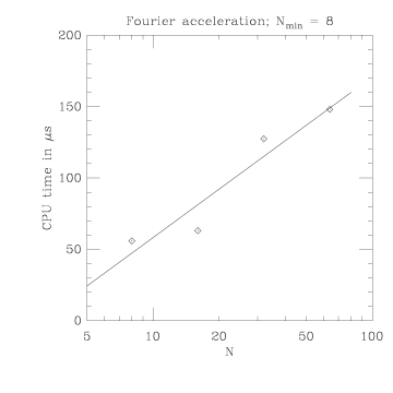
Figure 8:  Plot of CPU time $T_{gf}$ as a function of $N$ for the Fourier acceleration method. The solid line represents a least-squares fit to the ansatz $\,T_{gf}=A\,\log N\,+\,B\,$, with $\,A\,=\,48.91\,\pm\,0.11\,$ and $\,B\,=\,-54.42\,\pm\,0.45\,$ (both in microseconds).

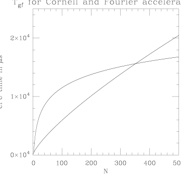
Figure 9:  Comparison between CPU times (divided by volume) as a function of the lattice size for the Cornell and the Fourier acceleration methods. The “almost” straight line corresponds to the Cornell method.

7.5 Conclusions

From our numerical simulations it is clear that the Fourier acceleration method is very effective in reducing critical slowing-down for the problem of $SU(2)$ Landau gauge fixing in two dimensions. On the other hand, its computational cost is much larger than that of the improved local methods, and therefore an accurate analysis should be always done to decide which method to use. The result of this analysis, as stressed in the previous subsection, will depend on the code, on the machine and on the condition used to stop the gauge fixing. From our data it seems that, at least up to lattice size of order $100$, the improved local methods should be always preferred.

From the point of view of computational cost, the Cornell method is clearly the best among the improved local methods. However, if the condition used to stop the gauge fixing is not (6.1), this conclusion could be different. In particular we saw that the stochastic overrelaxation is very effective in relaxing the value of the quantity $e_{6}\,$, defined in (4.8).

All the improved methods, including the Fourier acceleration, have the disadvantage of requiring tuning. However, the relations for the overrelaxation, the Cornell and the stochastic overrelaxation methods that were introduced in Section 5 and checked in Section 7.3 make the tuning of these methods simpler. Moreover, as reported in Section 6, the values of $\tau$ for the improved methods [for a fixed pair $(N,\beta)\,$] are much more stable than for the Los Alamos method. Therefore, in order to find the optimal choice of tuning parameter within a few per cent, it suffices to perform a few numerical tests.

Finally, from the discussion in Sections 4 and 7.2, it is clear that the quantities $e_{1}$–$e_{5}$ are essentially equivalent as a check of the goodness of the gauge fixing. Namely, when one of these quantities is measured, the evaluation of any of the others does not provide any new information. On the contrary, the quantity $e_{6}\,$ represents a more sensible check of the gauge-fixing condition and, in our opinion, should always be evaluated.

In a future paper [26] we will try to extend this analysis to the more interesting case of lattice gauge theory in four dimensions.

$N$	$\tau$	sweeps
$8$	$14.71\pm 0.68$	$330\pm 16$
$12$	$29.87\pm 1.14$	$600\pm 18$
$16$	$53.32\pm 2.00$	$1054\pm 34$
$20$	$86.55\pm 3.17$	$1650\pm 91$
$24$	$125.01\pm 7.32$	$2159\pm 79$
$28$	$157.22\pm 5.56$	$2797\pm 103$
$32$	$205.21\pm 8.03$	$3372\pm 105$
$36$	$282.78\pm 14.29$	$4389\pm 155$

Table 5:  The relaxation time and the number of sweeps for the Los Alamos method. Error bars are one standard deviation.

$N$	$\tau$	$\alpha$	sweeps	min. func.
$8$	$3.22\pm 0.30$	$0.489$	$86\pm 5$	$0.1171\pm 0.0012$
$12$	$4.54\pm 0.33$	$0.484$	$117\pm 6$	$0.0688\pm 0.0005$
$16$	$6.31\pm 0.63$	$0.481$	$152\pm 9$	$0.0430\pm 0.0003$
$20$	$6.92\pm 0.40$	$0.480$	$181\pm 8$	$0.0296\pm 0.0002$
$24$	$8.60\pm 0.53$	$0.482$	$217\pm 8$	$0.0218\pm 0.0001$
$28$	$9.52\pm 0.61$	$0.483$	$232\pm 9$	$0.0168\pm 0.0001$
$32$	$10.70\pm 0.43$	$0.484$	$260\pm 7$	$0.0134\pm 0.0001$
$36$	$11.65\pm 0.44$	$0.484$	$278\pm 7$	$0.0108\pm 0.0001$

Table 6:  The relaxation time, the coefficient $\alpha\,$, the number of sweeps and the value of the minimizing function for the Cornell method. Error bars are one standard deviation. The estimated error on the parameter $\alpha$ is about $0.002$ for all lattice sizes.

$N$	$\tau$	$\omega$	sweeps
$8$	$2.77\pm 0.35$	$1.72$	$77\pm 9$
$12$	$3.56\pm 0.15$	$1.77$	$95\pm 3$
$16$	$4.84\pm 0.20$	$1.83$	$136\pm 5$
$20$	$6.51\pm 0.32$	$1.86$	$208\pm 32$
$24$	$7.84\pm 0.38$	$1.88$	$208\pm 9$
$28$	$9.04\pm 0.52$	$1.90$	$249\pm 11$
$32$	$10.34\pm 0.62$	$1.90$	$257\pm 9$
$36$	$12.33\pm 0.61$	$1.92$	$306\pm 7$

Table 7:  The relaxation time, the coefficient $\omega$ and the number of sweeps for the overrelaxation method. Error bars are one standard deviation. The estimated error on the parameter $\omega$ is about $0.01$ for all lattice sizes.

$N$	$\tau$	$p$	sweeps
$8$	$3.35\pm 0.28$	$0.64$	$96\pm 5$
$12$	$4.38\pm 0.18$	$0.72$	$129\pm 4$
$16$	$6.48\pm 0.46$	$0.78$	$189\pm 11$
$20$	$7.84\pm 0.30$	$0.84$	$234\pm 7$
$24$	$9.47\pm 0.46$	$0.85$	$281\pm 13$
$28$	$11.28\pm 0.67$	$0.88$	$331\pm 13$
$32$	$12.67\pm 0.53$	$0.89$	$366\pm 12$
$36$	$14.95\pm 0.87$	$0.90$	$421\pm 15$

Table 8:  The relaxation time, the coefficient $p$ and the number of sweeps for the stochastic overrelaxation method. Error bars are one standard deviation. The estimated error on the parameter $p$ is about $0.02$ for all lattice sizes.

$N$	$\tau$	$\alpha$	sweeps
$8$	$3.08\pm 0.33$	$0.193$	$80\pm 7$
$16$	$3.30\pm 0.34$	$0.170$	$84\pm 7$
$32$	$3.11\pm 0.21$	$0.160$	$92\pm 8$
$64$	$3.46\pm 0.33$	$0.160$	$93\pm 9$

Table 9:  The relaxation time, the coefficient $\alpha\,$ and the number of sweeps for the Fourier acceleration method. Error bars are one standard deviation. The estimated error on the parameter $\alpha$ is about $0.003$ for all lattice sizes.

$N_{min}$	$z$		$c$		$\chi^{2}$
8	1.950 $\pm$	0.032	0.2441 $\pm$	0.0235	6.177 (	6 DF, level $=$	40.365 %)
12	1.986 $\pm$	0.042	0.2174 $\pm$	0.0284	4.443 (	5 DF, level $=$	48.751 %)
16	1.965 $\pm$	0.060	0.2332 $\pm$	0.0448	4.196 (	4 DF, level $=$	38.017 %)
20	1.919 $\pm$	0.090	0.2727 $\pm$	0.0810	3.718 (	3 DF, level $=$	29.353 %)
24	2.030 $\pm$	0.171	0.1857 $\pm$	0.1082	3.131 (	2 DF, level $=$	20.900 %)
28	2.281 $\pm$	0.238	0.0779 $\pm$	0.0636	0.819 (	1 DF, level $=$	36.551 %)
32	2.722 $\pm$	0.543	0.0164 $\pm$	0.0313	0.000 (	0 DF, level $=$	100.000 %)

Table 10:  Weighted least-squares fit for $\tau=c\,N^{z}$ at $N^{2}/\beta=32$, using lattice sizes $N\geq N_{min}$, for the Los Alamos method. Errors represent one standard deviation, and “DF” stands for “degrees of freedom”. Confidence level is the probability that $\chi^{2}$ would equal or exceed the observed value. The line in boldface marks our preferred fit.

$N_{min}$	$z$		$c$		$\chi^{2}$
8	0.854 $\pm$	0.049	0.5509 $\pm$	0.0877	1.134 (	6 DF, level $=$	98.002 %)
12	0.849 $\pm$	0.062	0.5611 $\pm$	0.1156	1.114 (	5 DF, level $=$	95.284 %)
16	0.825 $\pm$	0.089	0.6088 $\pm$	0.1833	0.977 (	4 DF, level $=$	91.329 %)
20	0.859 $\pm$	0.106	0.5409 $\pm$	0.1940	0.608 (	3 DF, level $=$	89.456 %)
24	0.762 $\pm$	0.168	0.7605 $\pm$	0.4401	0.045 (	2 DF, level $=$	97.759 %)
28	0.788 $\pm$	0.283	0.6936 $\pm$	0.6878	0.032 (	1 DF, level $=$	85.749 %)
32	0.721 $\pm$	0.471	0.8809 $\pm$	1.4627	0.000 (	0 DF, level $=$	100.000 %)

Table 11:  Weighted least-squares fit for $\tau=c\,N^{z}$ at $N^{2}/\beta=32$, using lattice sizes $N\geq N_{min}$, for the Cornell method. Errors represent one standard deviation, and “DF” stands for “degrees of freedom”. Confidence level is the probability that $\chi^{2}$ would equal or exceed the observed value. The line in boldface marks our preferred fit.

$N_{min}$	$z$		$c$		$\chi^{2}$
8	1.094 $\pm$	0.045	0.2390 $\pm$	0.0329	3.381 (	6 DF, level $=$	75.974 %)
12	1.120 $\pm$	0.048	0.2205 $\pm$	0.0325	1.062 (	5 DF, level $=$	95.745 %)
16	1.120 $\pm$	0.069	0.2202 $\pm$	0.0485	1.061 (	4 DF, level $=$	90.034 %)
20	1.063 $\pm$	0.108	0.2673 $\pm$	0.0949	0.577 (	3 DF, level $=$	90.157 %)
24	1.101 $\pm$	0.164	0.2340 $\pm$	0.1296	0.479 (	2 DF, level $=$	78.696 %)
28	1.239 $\pm$	0.301	0.1445 $\pm$	0.1513	0.185 (	1 DF, level $=$	66.707 %)
32	1.491 $\pm$	0.659	0.0590 $\pm$	0.1375	0.000 (	0 DF, level $=$	100.000 %)

Table 12:  Weighted least-squares fit for $\tau=c\,N^{z}$ at $N^{2}/\beta=32$, using lattice sizes $N\geq N_{min}$, for the overrelaxation method. Errors represent one standard deviation, and “DF” stands for “degrees of freedom”. Confidence level is the probability that $\chi^{2}$ would equal or exceed the observed value. The line in boldface marks our preferred fit.

$N_{min}$	$z$		$c$		$\chi^{2}$
8	1.048 $\pm$	0.043	0.3395 $\pm$	0.0449	3.673 (	6 DF, level $=$	72.089 %)
12	1.086 $\pm$	0.050	0.3002 $\pm$	0.0465	1.330 (	5 DF, level $=$	93.178 %)
16	1.034 $\pm$	0.081	0.3566 $\pm$	0.0940	0.680 (	4 DF, level $=$	95.377 %)
20	1.065 $\pm$	0.098	0.3217 $\pm$	0.1029	0.355 (	3 DF, level $=$	94.929 %)
24	1.084 $\pm$	0.171	0.3017 $\pm$	0.1751	0.338 (	2 DF, level $=$	84.455 %)
28	1.115 $\pm$	0.329	0.2702 $\pm$	0.3084	0.325 (	1 DF, level $=$	56.842 %)
32	1.407 $\pm$	0.609	0.0966 $\pm$	0.2062	0.000 (	0 DF, level $=$	100.000 %)

Table 13:  Weighted least-squares fit for $\tau=c\,N^{z}$ at $N^{2}/\beta=32$, using lattice sizes $N\geq N_{min}$, for the stochastic overrelaxation method. Errors represent one standard deviation, and “DF” stands for “degrees of freedom”. Confidence level is the probability that $\chi^{2}$ would equal or exceed the observed value. The line in boldface marks our preferred fit.

$N_{min}$	$z$		$c$		$\chi^{2}$
8	0.036 $\pm$	0.064	2.8513 $\pm$	0.6062	0.751 (	2 DF, level $=$	68.703 %)
16	0.040 $\pm$	0.102	2.8080 $\pm$	1.0094	0.748 (	1 DF, level $=$	38.712 %)
32	0.157 $\pm$	0.169	1.8020 $\pm$	1.1286	0.000 (	0 DF, level $=$	100.000 %)

Table 14:  Weighted least-squares fit for $\tau=c\,N^{z}$ at $N^{2}/\beta=32$, using lattice sizes $N\geq N_{min}$, for the Fourier acceleration method. Errors represent one standard deviation, and “DF” stands for “degrees of freedom”. Confidence level is the probability that $\chi^{2}$ would equal or exceed the observed value. The line in boldface marks our preferred fit.

References

- [1] J.E.Mandula and M.C.Ogilvie, Phys.Rev. D41 (1990) 2586; Ph. de Forcrand, J.E.Hetrick, A.Nakamura and M.Plewnia, Nucl.Phys. B (Proc. Suppl.) 20 (1991) 194; E.Marinari, C.Parrinello and R.Ricci, Nucl.Phys. B362 (1991) 487; P.Marenzoni and P.Rossi, Phys.Lett. B311 (1993) 219.
- [2] A.Nakamura and M.Plewnia, Phys.Lett. B255 (1991) 274.
- [3] A.Hulsebos, Nucl.Phys. B (Proc. Suppl.) 30 (1993) 539.
- [4] Ph. de Forcrand and J.E.Hetrick, Nucl.Phys. B (Proc. Suppl.) 42 (1995) 861.
- [5] M.L.Paciello, C.Parrinello, S.Petrarca, B.Taglienti and A.Vladikas, Phys.Lett. B289 (1992) 405; V.G.Bornyakov, V.K.Mitrjushkin, M.Müller-Preussker and F.Pahl, Nucl.Phys. B (Proc. Suppl) 34 (1994) 802.
- [6] K.G.Wilson, Recent Developments in Gauge Theories Proc. NATO Advanced Study Institute (Carges̀e, 1979), eds. G. ’t Hooft et al. (Plenum Press, New York - London, 1980).
- [7] J.E.Mandula and M.Ogilvie, Phys.Lett. B185 (1987) 127.
- [8] H.Suman and K.Schilling, Parallel Computing 20 (1994) 975.
- [9] O.Axelsson, Iterative Solution Methods (Cambridge University Press, Cambridge–New York–Melbourne, 1994).
- [10] W.H.Press, S.A.Teukolsky, W.T.Vetterling, B.P.Flannery, Numerical Recipes in Fortran (Cambridge University Press, Cambridge, 1992, second edition).
- [11] J.M.Ortega and W.C.Rheinboldt, Iterative Solution of Nonlinear Equations in Several Variables (Academic Press, New York, 1970).
- [12] R.Gupta, G.Guralnik, G.Kilcup, A.Patel, S.R.Sharpe and T.Warnock, Phys.Rev. D36 (1987) 2813.
- [13] Ph. de Forcrand and R.Gupta, Nucl.Phys. B (Proc. Suppl) 9 (1989) 516.
- [14] C.T.H.Davies, G.G.Batrouni, G.R.Katz, A.S.Kronfeld, G.P.Lepage, K.G.Wilson, P.Rossi and B.Svetitsky, Phys.Rev D37 (1988) 1581.
- [15] A.D.Sokal, Monte Carlo Methods in Statistical Mechanics: Foundations and New Algorithms, Cours de Troisième Cycle de la Physique en Suisse Romande (Lausanne, June 1989).
- [16] J.E.Mandula and M.Ogilvie, Phys.Lett. B248 (1990) 156.
- [17] J.Goodman and A.D.Sokal, Phys.Rev. D40 (1989) 2035.
- [18] A.Hulsebos, M.L.Laursen, J.Smit and A.J. van der Sijs, Nucl.Phys. B (Proc. Suppl) 20 (1991) 98.
- [19] A.Hulsebos, M.L.Laursen and J.Smit, Phys.Lett. B291 (1992) 431.
- [20] T.Draper and C.McNeile, Nucl.Phys. B (Proc. Suppl) 34 (1994) 777.
- [21] A.D.Sokal, Nucl.Phys. B (Proc. Suppl) 20 (1991) 55; U.Wolff, Nucl.Phys. B (Proc. Suppl) 17 (1990) 93.
- [22] L.Adler, Nucl.Phys. B (Proc. Suppl) 9 (1989) 437.
- [23] P.Marenzoni, G.Martinelli and N.Stella, Nucl.Phys. B (1995) 339.
- [24] H.Neuberger, Phys.Rev.Lett. 59 (1987) 1877.
- [25] U.Wolff, Phys.Lett. B288 (1992) 166.
- [26] A.Cucchieri and T.Mendes, in preparation.
- [27] K.G.Wilson, Phys.Rev. D10 (1974) 2445.
- [28] D.Zwanziger, Nucl.Phys, B412 (1994) 657.
- [29] F.R.Brown and T.J.Woch, Phys.Rev.Lett. 58 (1987) 2394.
- [30] M.L.Paciello, C.Parrinello, S.Petrarca, B.Taglienti and A.Vladikas, Phys.Lett. B276 (1992) 163.
- [31] C.Bernard, C.Parrinello and A.Soni, Phys.Rev. D49 (1994) 1585.
- [32] H.G.Dosch and V.F.Müller, Fortschr.Phys. 27 (1979) 547.
- [33] S.L.Adler, Phys.Rev. D37 (1988) 458.
- [34] M.Creutz, Phys.Rev. D21 (1980) 2308.
- [35] R.G.Edwards, S.J.Ferreira, J.Goodman and A.D.Sokal, Nucl.Phys. B380 (1992) 621.