HLRZ 66/95

GUTPA/95/10/05

November 1995

Non-compact Lattice QED
with Two Charges:
Phase Diagram and Renormalization Group Flow

A. Ali Khan

Department of Physics and Astronomy, University of Glasgow,

Glasgow G12 8QQ, UK

The phase diagram of non-compact lattice QED in four dimensions with staggered fermions of charges 1 and $-1/2$ is investigated. The renormalized charges are determined and found to be in agreement with perturbation theory. This is an indication that there is no continuum limit with non-vanishing renormalized gauge coupling, and that the theory has a validity bound for every finite value of the renormalized coupling. The renormalization group flow of the charges is investigated and an estimate for the validity bound as a function of the cut-off is obtained. Generalizing this estimate to all fermions in the Standard Model, it is found that a cut-off at the Planck scale implies that $\alpha_{R}$ has to be less than $1/80$. Due to spontaneous chiral symmetry breaking, strongly bound fermion-antifermion composite states are generated. Their spectrum is discussed.

1 Introduction

Interest in non-perturbative investigations of QED has a long history. From perturbation theory there are indications (Landau pole [1]) that the cut-off can only be removed from the theory if the renormalized charge vanishes. Also, it is a yet unsolved fundamental question [2], why the fine structure constant has the value $\alpha\simeq 1/137$. At strong coupling, QED exhibits a chiral symmetry breaking phase transition of 2nd order [3, 4, 5, 6], where tightly bound fermion-antifermion pairs are generated. There one could expect a deviation from the charge screening behaviour known from perturbative QED. The phase transition makes strongly coupled $U(1)$ gauge theories interesting also for applications in technicolour theories because of large anomalous dimensions of the operator $\bar{\psi}\psi$ [7]. For several years, the possibility of a non-trivial continuum limit, or a non-trivial ultraviolet-stable fixed point of the Callan-Symanzik $\beta$ function, has been investigated in the non-compact formulation of QED on the lattice (see for example [9]–[16]).

Studying non-compact lattice QED with dynamical fermions, some groups find non-trivial scaling behaviour [12, 17, 18], others find their critical exponents to indicate triviality [13, 19]. The QED $\beta$ function has been studied non–perturbatively on the lattice [15, 20], and using Schwinger-Dyson equations [21]. It turns out to be in agreement with perturbation theory and to show no indications of a non-trivial fixed point. If QED is trivial in the limit of infinite cut-off, there is a maximal cut-off corresponding to every finite value of the renormalized charge. One is interested in the size of this validity bound. A rough estimate of it has been made in a lattice study of QED with one charge [15].

In nature one finds several differently charged types of fermions. In the presence of several charges, new non-perturbative phenomena may arise which could affect the phase structure. An important question is whether chiral symmetry breaking sets in at the same value of the bare coupling for all fermions or whether some fermion species can be massless and others in the chirally broken phase at the same time. The phase diagram of such a system has to be investigated with respect to a physically interesting continuum limit. In QED with one charge, neutral pointlike Goldstone bosons and scalar particles are generated due to the chiral symmetry breaking phase transition. One could expect that in the two-charge model  there is a larger number of neutral pointlike bound states which could in principle carry colour charge and have an effect on the $\beta$ function of QCD. Moreover, electrically charged bound states may appear which could change the behaviour of the QED $\beta$ function and push the validity bound towards much lower energies. It is of interest to see whether charge renormalization is in agreement with perturbation theory and which states give relevant contributions.

To investigate non-perturbative phenomena in the coupling between different species of fermions, a model with two species of staggered fermions with a ratio of their charges of $-1/2$ (‘two-charge model’) was studied, comparable to $u$ and $d$ quarks whose strong and weak interactions are switched off.

In section 2 of this paper a description of the model and details of the simulation are given. The phase diagram, obtained from the chiral condensates, and the scaling behaviour are discussed. The charged sector of the model is presented in section 3. The renormalized charges are determined non-perturbatively using current-photon correlation functions and are compared with renormalized lattice perturbation theory. There is good agreement which leads to the conclusion that the model is trivial. Using perturbation theory, the renormalization group flow of the charges is determined, which leads to an estimate of the validity bound resulting from triviality. Spectrum and renormalization group flows of fermion-antifermion composite states are discussed in section 4.

2 Phase diagram and scaling behaviour

2.1 Action and Simulation Details

The ‘two-charge model’ contains a non-compact gauge field with the action

$$S_{g}=\frac{\beta}{2}\sum_{x}\sum_{\mu<\nu}F_{\mu\nu}^{2}(x),$$ (1)

$$F_{\mu\nu}(x)=\Delta_{\mu}A_{\nu}(x)-\Delta_{\nu}A_{\mu}(x),$$ (2)

and two sets with each four flavours of staggered fermions which couple to the gauge fields with couplings 1 and –1/2, corresponding to $u$ and $d$ quarks with only electromagnetic interactions:

$$S_{f}=\sum_{x,y}\left\{\bar{\chi}_{u}(x)M_{u,xy}\chi_{u}(y)+\bar{\chi}_{d}(x)M_{d,xy}\chi_{d}(y)\right\}.$$ (3)

The coupling $\beta$ is related to the bare electric charges $e_{k}$ by $\beta=1/(c_{k}e_{k})^{2}$, $k=1,2$. The lattice spacing $a$ is set to 1. The fermion matrices are given by

$$M_{k,x,y} = D_{k,xy}+m_{k}\delta_{xy}$$

$$D_{k,xy}(x) = \frac{1}{2}\sum_{\mu}\eta_{\mu}(x)\left\{e^{c_{k}iA_{\mu}(x)}\delta_{y,x+\hat{\mu}}-e^{-c_{k}iA_{\mu}(y)}\delta_{y,x-\hat{\mu}}\right\};$$ (4)

$$k=u,d c_{u}=1,\;c_{d}=-1/2.$$ ;

In the limit $m_{d}\rightarrow\infty$ this model goes over into non-compact QED with one charge [9, 14]. For the gauge fields, periodic boundary conditions in all four directions were chosen, for the fermions periodic spatial and antiperiodic temporal boundary conditions. The simulations were performed on lattices of size $8^{3}\times 12$. From simulations with one charge, one expects that for the chosen values of $\beta$, $m_{u}$ and $m_{d}$ finite size effects are small [15]. For each simulated point $(\beta,m_{u},m_{d})$ $O(1000)$ configurations in equilibrium were generated using a Hybrid Monte Carlo algorithm. Every fifth was stored for spectrum and charge calculations.

Staggered fermions are a useful choice for studying chiral symmetry properties at finite lattice spacing. The action (3) of the two-charge model has for the $k$th species of fermions a chiral $U(1)_{V}\times U(1)_{A}$ symmetry, if $m_{k}=0$. The order parameters are the chiral condensates

$$\sigma_{k}\equiv\langle\bar{\chi}_{k}\chi_{k}\rangle=-\langle TrM^{-1}_{k}\rangle,$$ (5)

which are computed using a stochastic estimator [22]. Simulation results for the chiral condensates are shown in tables 1 and 2.

2.2 Determination of the critical points

In non-compact QED with one set of staggered fermions the chiral condensate $\sigma$ is consistent with a mean field like equation of state with logarithmic corrections motivated from a linear $\sigma$ model [15, 23]. The parameters in the equation of state are expanded in a power series in the reduced coupling $(1-\beta/\beta_{c})$, where $\beta_{c}$ denotes the critical coupling. The logarithmic corrections are only expected to become important very close to the critical point due to renormalization effects. It is expected that they become relevant also here if one goes closer to the critical point. From the results in tables 1 and 2, and as illustrated for $\beta=0.18$ in figure 1, it appears that the chiral condensates are fairly independent of the other fermion’s bare mass.

Figure 1: Dependence of $\sigma_{u}$ on $m\equiv m_{d}$ (left) and of $\sigma_{d}$ on $m\equiv m_{u}$ (right). Circles denote $m$ = 0.02, squares $m$ = 0.04 and diamonds $m$ = 0.09. $\beta=0.18$. Statistical errors are smaller than the symbols.

Thus to determine the critical points in the two-charge model  an Ansatz with two uncoupled mean field like equations of state with logarithmic corrections for each fermion is used:

$$m_{k}=2\tau_{k}\frac{\sigma_{k}}{\ln^{p_{k}}|\sigma_{k}^{-1}|}+4\theta_{k}\frac{\sigma_{k}^{3}}{\ln|\sigma_{k}^{-1}|},\;\;k=u,d.$$ (6)

For the determination of the renormalization group flow it is desirable to know the chiral condensates as a function of $(\beta,m_{u},m_{d})$ in the whole parameter space. It turns out to be possible to approximate the chiral condensates for all $\beta$ with equations of state (6), using the following expansion of the couplings:

$$\tau_{u}/\theta_{u} = \tau_{u}^{(1)}(1-\beta/\beta_{cu})+\tau_{u}^{(3)}(1-\beta/\beta_{cu})^{3},$$

$$1/\theta_{u} = \theta_{u}^{(0)}+\theta_{u}^{(1)}(1-\beta/\beta_{cu})+\theta_{u}^{(3)}(1-\beta/\beta_{cu})^{3},$$ (7)

and

$$\tau_{d}/\theta_{d} = \tau_{d}^{(1)}(1-\beta/\beta_{cd}),$$

$$1/\theta_{d} = \theta_{d}^{(0)}+\theta_{d}^{(1)}(1-\beta/\beta_{cd}).$$ (8)

Figure 2: Chiral condensates (open symbols: $\sigma_{u}$, filled symbols: $\sigma_{d}$) as a function of $\beta$ with a mean field fit with logarithmic corrections. Triangles correspond to $m_{k}$ = 0.02, squares to $m_{k}$ = 0.04, asterisks to $m_{k}$ = 0.09 and circles to $m_{k}$ = 0.16, $k=u,d$. The solid lines show the result of the fits and the dashed lines solutions of the equations of state with $m_{k}$ set to 0.

$\beta_{ck}$, $\tau_{k}^{(1,3)}$, $\theta_{k}^{(0,1,3)}$ and $p_{k}$ are fit parameters. Including all results for $\sigma_{u}$ simulated at $m_{u}\leq 0.09$, one obtains $\beta_{cu}$ = 0.173. Values of the fit parameters and the fit errors are listed in table 3. For a fit of $\sigma_{d}$ all results with $\beta\leq 0.1$ and $m_{d}\leq 0.09$ have been used, and the critical coupling is $\beta_{cd}=0.047$. From varying the range of the chiral condensates included in the fit, one estimates the error on $\beta_{cu}$ and $\beta_{cd}$ to be approximately 0.001, which is larger than the fit error. Without including logarithmic corrections, $\beta_{cu}$ comes out to be $0.183(1)$ and $\beta_{cd}$ to be $0.049(1)$ [25]. The cubic term in eq. (7) is included to obtain an approximate description of $\sigma_{u}$ also in the region where $\beta\sim\beta_{cd}$. It has been checked that with a fit in the range $0.16\leq\beta\leq 0.22$, including only linear terms in the reduced coupling, one obtains the same result for $\beta_{cu}$ within errors. As seen in figure 2, eqs. (6) give a good description for the chiral condensates in the range of couplings $\beta\geq 0.05$. Two or three of the same symbols lying on top of each other at the $\beta$ values 0.06, 0.16, 0.18, 0.20 and 0.21 corresponds to simulations at various values of $m_{u}$ at a fixed value of $m_{d}$ or vice versa. One further notices that in the regions where the $d$ fermion undergoes a transition, the $u$ fermion is that far in the broken region that $\sigma_{u}$ is practically independent of $m_{u}$ (as well as of $m_{d}$).

2.3 Renormalized fermion masses

The next step in the investigation of the critical behaviour is the determination of the renormalized fermion masses or inverse fermionic correlation lengths. Because the fermions are charged, their correlation functions are gauge dependent. For the calculation of their expectation value, a technique as described in references [26, 15] is used. First, Landau gauge is fixed by imposing the following gauge fixing condition:

$$\sum_{\mu}\bar{\Delta}_{\mu}\,A_{\mu}(x)=0,$$ (9)

where $\bar{\Delta}_{\mu}$ denotes the backward derivative on the lattice. An additional gauge-like degree of freedom is the invariance of the action under the local transformation

$$A_{\mu}(x) \to A_{\mu}(x)+\Delta_{\mu}\,\alpha(x),$$

$$\chi(x) \to \mbox{e}^{-ic_{k}\alpha(x)}\chi_{k}(x),$$

$$\bar{\chi}_{k}(x) \to \mbox{e}^{{i}c_{k}\alpha(x)}\bar{\chi}_{k}(x),$$ (10)

with

$$\alpha(x)=\sum_{\mu}\frac{4\pi}{L_{\mu}}n_{\mu}x_{\mu}\;,n_{\mu}\in{{Z}},$$ (11)

where $L_{\mu}$ is the lattice extent in the $\mu$ direction.

Figure 3: $u$ fermion propagators at $\beta=0.16$ and $m_{u}=m_{d}=0.02$. Crosses correspond to positive values of the correlation function, squares to negative values. Solid lines denote the fit.

Figure 4: $d$ fermion propagators at $\beta=0.16$ and $m_{u}=m_{d}=0.02$. The meaning of the symbols is explained above.

The lattice average of the gauge field

$$\bar{A}_{\mu}=\frac{1}{V}\sum_{x}A_{\mu}(x),\;V=\prod_{\mu}L_{\mu},$$ (12)

has a nonvanishing expectation value on our (relatively small) ensembles. By shifting it by multiples of $4\pi/L_{\mu}$, such that it is restricted to the interval $(-2\pi/L_{\mu},2\pi/L_{\mu}]$, this additional degree of freedom was fixed. In the two-charge model  this interval is chosen twice as large as in a model with fermions of charge 1. This is necessary to preserve also the boundary conditions of the $d$ fermion, which couples with charge $-1/2$. $\bar{A}_{\mu}$ is approximately constant over $O(10-20)$ configurations. Following the procedure described in [26, 15], the set of data samples at each parameter value was divided into subsets of 10-20. The correlation functions were averaged over each subset and fitted with the free form of a staggered fermion propagator in a constant background field $B_{\mu}$. For the $u$ fermion, $B_{\mu}$ agrees with the expectation value of $\bar{A}_{\mu}$, taken over the given subset, for the $d$ fermion with the expectation value of $-\bar{A}_{\mu}/2$. The fits were performed with the routine MINUIT. The Ansatz gives a good description of the data. An example for this is shown in figure 4. Results are given in tables 4 and 5. Another indication that the fermion correlation functions behave simliar to free propagators with a renormalized mass $m_{u,dR}$, is obtained by comparing the simulation data for the chiral condensates with free propagator expressions:

$$\langle\bar{\chi}_{k}\chi_{k}\rangle=\frac{1}{V}\sum_{p_{\mu}}\frac{m_{kR}}{\sum_{\mu}\sin^{2}p_{\mu}+m_{kR}^{2}},\;k=u,d,$$ (13)

with the lattice momenta

$$p_{i} = \frac{2\pi}{L_{i}}n_{i},\;n_{i}=1,\ldots,L_{i},\;i=1,\ldots,3;$$

$$p_{4} = \frac{\pi}{L_{4}}(2n_{4}-1),\;n_{4}=1,\ldots,L_{4},\;$$

Figure 5: Chiral condensate $\langle\bar{\chi}_{u}\chi_{u}\rangle$ for $\beta\geq 0.14$ plotted against the renormalized mass $m_{uR}$. The line denotes eq. (13).

Figure 6: Chiral condensate $\langle\bar{\chi}_{d}\chi_{d}\rangle$ plotted against $m_{dR}$. The line denotes eq. (13).

Figures 6 and 6 show that for small masses the results agree quite well with eqs. (13). The fermion wave function renormalization constant is $O(1)$. Since $m_{kR}\propto\langle\bar{\chi}_{k}\chi_{k}\rangle$ for small $m_{kR}$, eqs. (6) and (7) imply that near $\beta\simeq\beta_{cu}$ the renormalized $u$ mass scales according to

$$m_{uR}\ln^{-1/3}(m_{uR}^{-1})\propto m_{u}^{1/3},$$ (14)

and the renormalized $d$ mass according to

$$m_{dR}\ln^{-p_{d}}(m_{dR}^{-1})\propto m_{d}.$$ (15)

The scaling behaviour of the $d$ is thus in this region close to the perturbative behaviour, which is very different from the behaviour of the $u$ fermion in this region. For very large $\beta$ both renormalized masses follow eq. (15). In the neighbourhood of $\beta\simeq\beta_{cd}$, eqs. (6) and (7) indicate that

$$m_{dR}\ln^{-1/3}(m_{dR}^{-1})\propto m_{d}^{1/3}.$$ (16)

In this region the difference between the bare and renormalized masses of the $d$ becomes small.

2.4 Phase Diagram

Figure 7 shows a sketch of the phase diagram. The agreement of the results with eq. (6) suggests that there are two distinct regions of chiral symmetry breaking for both fermion species. This does not correspond to the expectations in a confining theory. If chiral symmetry breaking in non-compact QED was related to confinement, one would expect both species of fermions to develop chiral condensates in the same time. The end points of the phase boundary of the $u$, which separates the symmetric phase of the $u$ on the $m_{u}=0$ surface from its broken phase, are given by $\beta_{cu}$ and $\beta_{c}$, the critical point of QED with one set of $u$ fermions [15] which is the limit of the two-charge model if $m_{d}\rightarrow\infty$. In the presence of more charges, the critical point is shifted towards stronger coupling, so $\beta_{cu}$ is slightly smaller than $\beta_{c}$. In the limit $m_{u}\rightarrow\infty$, which corresponds to QED with one set of charges with coupling $\beta=4/e^{2}$ one expects this to occur at $\beta_{c}/4$ ($\sim 0.046$, using the result of [15]). In the two-charge model a value very close to this is obtained, $\beta_{cd}\simeq 0.047$. Below $\beta_{cu}$, no continuum limit with two fermion species is possible. For the investigated parameter values at $\beta\leq 0.14$, the renormalized $u$ masses are $O(1)$ in lattice units, which means the $u$ fermion is in this region practically not present in the spectrum. In the region $\beta\mathchar 13350\relax\beta_{cu}$ both fermion masses can go to zero, so this region is the most interesting candidate for a continuum limit of the model.

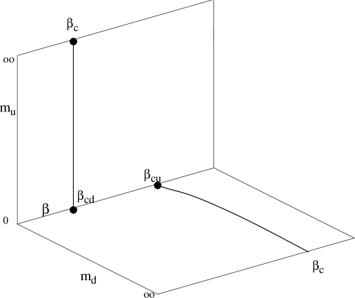
Figure 7: Sketch of the phase diagram.

3 The renormalized coupling

3.1 Charge determination on the lattice

The Ward identities ensure that the charge renormalization is entirely determined by the wave function renormalization of the photon:

$$e_{u,d\,R}^{2}=Z_{3}\>e_{u,d}^{2}.$$ (17)

$Z_{3}$ is given by the zero momentum limit of the gauge invariant part of the photon propagator:

$$D(k) = \frac{\beta}{N_{k}V}\sum_{\stackrel{{\scriptstyle\scriptstyle\mu,k|k^{2}={\rm const},}}{{{k_{\mu}=0}}}}\hat{k}^{2}\left.\langle\tilde{A}_{\mu}(\hat{k})\tilde{A}_{\mu}(-\hat{k})\rangle\right|_{k_{\mu}=0},$$ (18)

$$Z_{3} = \lim_{k\rightarrow 0}D(k).$$ (19)

The sum in eq. (18) runs over all directions $\mu$ and for each $\mu$ over all $N_{k}$ choices of $k$ with fixed $k^{2}$ and $k_{\mu}=0$. Due to the lattice, the momenta enter the photon propagator as

$$\hat{k}_{\mu}=e^{ik_{\mu}}-1\;\mbox{and}\;\hat{k}^{2}=\hat{k}_{\mu}{\hat{k}}^{\ast}_{\mu}.$$ (20)

The right hand side of (18) turns out to be strongly fluctuating and inappropriate for an extrapolation to $k\rightarrow 0$. Thus for the calculation of $D(k)$ a method analogous to references [14, 15, 27] is used. The photon propagator $D(k)$ is re-expressed using the Ward identities [28] in terms of a correlator between the gauge field and the fermion current:

$$D(k)=1-\left.\frac{1}{N_{k}V}\sum\left\langle\tilde{j_{\mu}}(\hat{k})\tilde{A_{\mu}}(-\hat{k})\right\rangle\right|_{k_{\mu}=0},$$ (21)

where in the two-charge model

$$j_{\mu}(x)=\frac{\delta}{\delta A_{\mu}(x)}\sum_{yz}\left\{(\bar{\chi}_{u}(y)M_{u,yz}\chi_{u}(z)+\bar{\chi}_{d}(y)M_{d,yz}\chi_{d}(z)\right\}.$$ (22)

The correlator in eq. (21) has less fluctuations and could be used for an extrapolation of $D(k)$ to $k\rightarrow 0$. The fermion current was computed using a stochastic estimator with 30-75 inversions of the fermion matrices.

3.2 Comparison with perturbation theory

Taking contributions of both fermions into account, in one-loop perturbation theory the vacuum polarization tensor has the following form:

$$1/\beta\;\Pi_{\mu\nu}(k,m_{uR},m_{dR},V)=e_{u}^{2}\;\Pi^{(1)}_{\mu\nu}(k,m_{uR},V)+e_{d}^{2}\;\Pi^{(1)}_{\mu\nu}(k,m_{dR},V),$$ (23)

where $\Pi^{(1)}_{\mu\nu}(k,m_{R},V)$ is the vacuum polarization tensor for a single set of fermions with the renormalized mass $m_{R}$ on a lattice of volume $V$. Projection onto the gauge invariant part yields

$$D(k) = 1+e_{u}^{2}\,\Pi^{(1)}(k,m_{uR},V)+e_{d}^{2}\,\Pi^{(1)}(k,m_{dR},V),$$ (24)

where $\Pi^{(1)}(k,m_{R},V)$ is the one loop vacuum polarization function for one set of staggered fermions:

$$\Pi^{(1)}(k,m_{R},V)={1\over{\hat{k}^{2}}}\left.\left[\Pi_{\mu\mu}^{(1)}(k,m_{R},V)-\Pi_{\mu\mu}^{(1)}(0,m_{R},V)\right]\right|_{k_{\mu}=0}.$$ (25)

The second term on the right hand side occurs because $\Pi_{\mu\mu}^{(1)}(0,m_{R},V)\neq 0$ for a finite $V$. This would correspond to a finite photon mass, and the term is subtracted off. Here, a fixed $\mu$ has been chosen with $k_{\mu}=0$. Finally one obtains for the photon propagator in the two-charge model:

$$\frac{\beta}{D(k)}=\beta_{R}+\Pi(0,m_{uR},m_{dR},\infty)-\Pi(k,m_{uR},m_{dR},V).$$ (26)

Extrapolating this to $V\rightarrow\infty,k\rightarrow 0$:

$$\beta_{R}=\beta-\Pi(0,m_{uR},m_{dR},\infty),$$ (27)

gives the perturbative relation between the bare and the renormalized coupling. Combining the last two expressions, one gets the fit formula for the Monte Carlo results for $D(k)$:

$$\frac{\beta}{D(k)}=\beta_{R}+\Pi(0,m_{uR},m_{dR},\infty)-\Pi(k,m_{uR},m_{dR},V).$$ (28)

The renormalized coupling $\beta_{R}$ is the only free parameter in the fit.

Figure 8: Photon propagator, $\beta$ = 0.17, $m_{u}$ = $m_{d}$ = 0.02. The circles describe the data and the asterisks the fit with the perturbative formula. The extrapolation to $k\rightarrow 0$ is denoted by an asterisk. The variable $K2$ on the x axis is defined as $K2=576/(2\pi)^{2}k^{2}$ to be an integer.

For the calculation of $\Pi(0,m_{uR},m_{dR},\infty)$, the effect of the zero modes $\bar{A}_{\mu}$ of the gauge field has to be taken into account. Their contribution is important where fermions are light, as are the $d$ fermions at the simulated parameter values with $\beta\sim\beta_{cu}$. To calculate the perturbative vacuum polarization functions, the background fields are integrated over:

$$\Pi(k,m_{uR},m_{dR},V)=\frac{\int d^{4}\bar{A}\det(D_{u}+m_{u})\det(D_{d}+m_{d})\sum_{p}\rho(p,k,\bar{A},m_{uR},m_{dR},V)}{\int d^{4}\bar{A}\det(D_{u}+m_{u})\det(D_{d}+m_{d})}.$$ (29)

Also in the presence of constant background fields the fermion determinant of free fermions can be written as a product of contributions with definite momentum:

$$\det M_{i}=\det(D_{i}+m_{i})=\prod_{k_{i}}\left[m_{i}^{2}+\sum_{\mu}\sin^{2}(k_{i,\mu}+c_{i}\bar{A}_{\mu})\right]^{\frac{1}{2}}\!,\;i=u,d,$$ (30)

with $c_{u}$ = 1 and $c_{d}=-1/2$. Choosing $\mu=3$ in eq. (25) the function $\rho$ looks as follows:

$$\rho = \sum_{i=u,d}\left[-2\frac{\sum_{\mu\neq 3}\left(\cos(\tilde{k}_{i,\mu})\sin(p_{\mu}/2)\right)^{2}}{D(\tilde{k}_{i}-p,m_{iR})D(\tilde{k}_{i}+p,m_{iR})}\right.$$ (31)

$$\!\!\left.\vphantom{\frac{1}{2}}+{\textstyle\sin^{2}\left((\tilde{k}_{i,3}-p_{3})/2\right)}\!\left\{\frac{1}{D(\tilde{k}_{i}-p,m_{iR})}-\frac{1}{D(\tilde{k}_{i}+p,m_{iR})}\right\}^{2}\right]\cos^{2}(\tilde{k}_{i,3}),$$

where

$$D(k,m_{R})=m_{R}^{2}+\sum_{\mu}{\textstyle\sin^{2}(k_{\mu}/2)}$$ (32)

and

$$\tilde{k}_{u}=k_{u}+\bar{A}\;\mbox{and}\;\tilde{k}_{d}=k_{d}-\bar{A}/2.$$ (33)

The integral over the background fields was evaluated using a Monte Carlo method, representing the background fields through Gaussian random numbers and calculating the weight of the fermion determinant in the presence of these background fields. Figure 8 shows an example for a fit of $D(k)$ with one-loop perturbation theory in the presence of background fields. The oscillations of $D(k)$ are caused by the dependence of $k$ on the direction due to the asymmetry of the lattice. The renormalized couplings are listed in tables 4 and 5.

The renormalized coupling can be calculated directly in perturbation theory, using eq. (27). One would like to compare the data with the perturbative result. Since this is of interest especially in regions of a high cut-off, i.e. for small masses, the limit $m_{uR},m_{dR}\ll 1$ of the vacuum polarization function (27) is taken, which gives

$$\beta_{R}-\beta=-\Pi(0,m_{uR},m_{dR},\infty)=-\frac{1}{6\pi^{2}}\ln(m_{uR}^{4}m_{dR})+5c/4.$$ (34)

From QED with one species of fermions with charge 1, it is known that $c\simeq 0.0210$ [15]. Figure 9 shows that in the small mass limit the renormalized charges indeed follow the logarithmic behaviour as in the right hand side of eq. (34). For larger masses, $\Pi$ is no more a function of $m_{uR}^{4}m_{dR}$ alone, but the simulation results are still in agreement with perturbation theory [30]. There does not seem to be an effect on charge renormalization from possible charged bound states.

Figure 9: Renormalized couplings in the region of small $m_{uR}$ and $m_{dR}$. The line denotes the small mass limit of one-loop perturbation theory.

The agreement with perturbation theory indicates that this model is trivial in the limit of infinite cut-off, and that all renormalized charges vanish if only one fermion mass goes to zero. The renormalized coupling vanishes in those parts of the phase diagram (see figure 7) where $\sigma_{u}$ or $\sigma_{d}$ equal zero.

One would now like to find a relation between a finite renormalized coupling and a corresponding cut-off. The ratio of the renormalized masses has to be kept constant while the cut-off is varied. Re-expressing (34) in terms of $R=m_{uR}/m_{dR}$ and exponentiating, one obtains:

$$m_{uR}=1.365\>R^{\frac{1}{5}}\exp{\left(-\left[\frac{6\pi^{2}}{5}(\beta_{R}-\beta)\right]\right)}.$$ (35)

From this equation one will be able to estimate the maximal cut-off belonging to each renormalized charge. For this, one needs to know which $\beta$ coordinate the point with maximal cut-off on a renormalization group flow  line with fixed $\beta_{R}$ and $R$ has. This flow line will be the intersection between the surface with fixed $R$ and the one with fixed $\beta_{R}$ in the three dimensional parameter space.

3.3 Renormalization group flow of the coupling

It is not feasible to cover all the regions of the phase diagram that are of interest with simulations. For a determination of the renormalization group flows of the charge one therefore has to make use of extrapolation methods. If one is able to find a functional dependence of the renormalized mass on the bare parameters it is possible to calculate the renormalized coupling using perturbation theory from eq. (27). The chiral condensates can be approximated as functions of $\beta$, $m_{u}$ and $m_{d}$ through the equations of state. Figures 6 and 6 suggest that the renormalized masses can be expressed as functions of the chiral condensate, where for small masses there is agreement with the free propagator relation eq. (13), and the leading term is linear. For the renormalization group flows one is primarily interested in regions where both fermion masses are smaller than 1, so $m_{uR}$ is fitted for $\beta\geq 0.14$ with the Ansatz

$$m_{uR} = P_{1}\langle\bar{\chi}_{u}\chi_{u}\rangle+P_{2}\langle\bar{\chi}_{u}\chi_{u}\rangle^{3}.$$ (36)

Here, $\chi^{2}$ per degree of freedom is 1.5. The following fit gives a good description for the $d$ mass for $\beta\geq 0.14$:

$$m_{dR} = Q_{1}\langle\bar{\chi}_{d}\chi_{d}\rangle,$$ (37)

with $\chi^{2}$ per degree of freedom equal to 2.2. A cubic term is not needed here. The fit parameters $P$ and $Q$ are given in table 6. As illustrated in figure 10, one thus obtains a good description for the renormalized masses.

Figure 10: Renormalized masses as a function of the chiral condensates. The squares denote simulation results and lines the fit according to eqs. (36) and (37), respectively.

To obtain the renormalized masses as a function of the bare parameters, first the equations of state were solved explicitly for the chiral condensates using Müller’s method [31] for calculating zeros of non-linear functions. The results were thus inserted into the fit equations (36) and (37) respectively.

Using this method, a grid of values for the mass ratio $R$ in the phase diagram is generated and, using renormalized perturbation theory, also for $\beta_{R}$. Using a graphics package, surfaces of constant $\beta_{R}$ and $R$ can be drawn. Figure 11 shows a surface $S_{\beta_{R}}$ (black) with a constant $\beta_{R}$ and its intersection with a surface $S_{R}$ (grey) of constant $R$ of $O(1)$.

For large $m_{u}$ and $m_{d}$ both renormalized fermion masses are large. Therefore $\beta_{R}\sim\beta$, which implies that surfaces with fixed $\beta_{R}$ are nearly perpendicular to the $\beta$ axis. The behaviour at small $m_{u}$, $m_{d}$ can be read off from eq. (34). If $m_{u}$ is lowered, the surfaces bend over until they end on the $m_{u}=0$ plane below the line where the chiral symmetry of the $u$ fermion is broken. The larger $\beta_{R}$ is, the closer the end line of the surface on the $m_{u}=0$ plane comes to the critical line of the $u$, except for very small $m_{d}$. In a whole range of $\beta<\beta_{cu}$ and small bare masses, $m_{dR}$ is much smaller than $m_{uR}$ and for constant $m_{d}$ nearly constant. So surfaces with constant $\beta_{R}$ bend at small $m_{d}$ towards small $\beta$, as the black surface in figure 11 indicates. They intersect the $m_{d}=0$ plane in the broken phase of the $d$ fermion, and thus cut the $\beta$ axis at $\beta<\beta_{cd}$. The important point to note is that $S_{\beta_{R}}$ intersects the surfaces $m_{u}=0$ or $m_{d}=0$ only in regions where both renormalized fermion masses are non-zero.

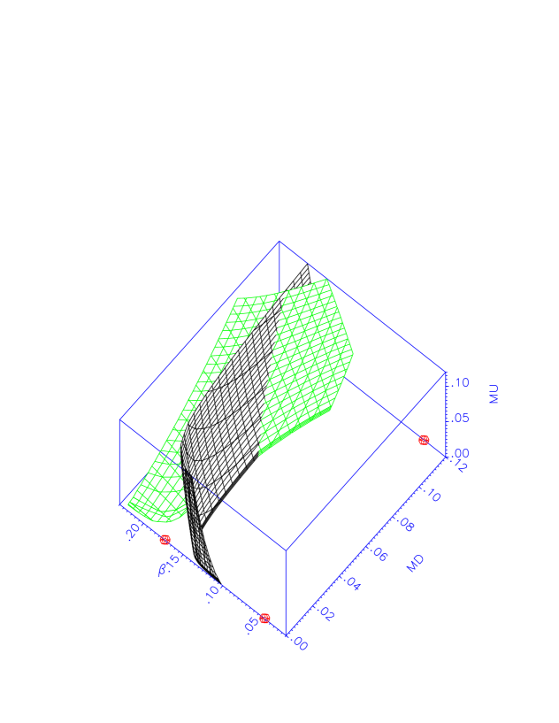
Figure 11: Surfaces with $\beta_{R}=0.27$ (black) and $R=5$ (grey). The little spheres denote $\beta_{cu}$ and $\beta_{cd}$.

Surfaces of constant $R$ end for $\beta\geq\beta_{cu}$ on the $\beta$ axis. The scaling behaviour of the masses in eqs. (14) and (15) implies that at $\beta=\beta_{cu}$ these surfaces obey the relation $m_{u}\sim cm_{d}^{3}$, where $c$ is a constant. If $\beta$ is lowered past $\beta_{cu}$, $m_{uR}$ increases quickly. As indicated in figure 11, the end line of the surfaces with constant $R$ on the $m_{u}=0$ plane therefore has to turn away from the $\beta$ axis towards a finite $m_{d}$. For an estimate of the validity bound, the intersection line of both surfaces is of interest, as it represents a flow line where both $R$ and $\beta_{R}$ are constant while the cut-off scale is changed. It ends on the $m_{u}=0$ plane at $\beta<\beta_{cu}$. As one moves down along the intersection line, the cut-off becomes larger, but never reaches infinity.

3.4 Validity bound

In non-compact QED with four flavours of staggered fermions of charge 1, the $\beta$ function goes, in the limit of small renormalized mass, over into the prediction of one loop continuum perturbation theory for four fermion flavours of charge 1 [15]. In the two-charge model  with four flavours of charge 1 and four flavours of charge $-1/2$, a corresponding relation is fulfilled (34). This suggests that in the presence of $N$ species of fermions the renormalized charge can be approximated with the formula

$$\beta_{R}-\beta=-\sum_{i=1}^{N}\frac{Q_{i}^{2}}{6\pi^{2}}\ln\left(am_{iR}\right)+\sum_{i=1}^{N}Q_{i}^{2}c.$$ (38)

In this section the lattice spacing $a$ is kept explicitly, to illustrate the dependence on the cut-off. In QED with one charge and in the two-charge model it was reasonable to approximate the bare charge corresponding to the point of maximal cut-off by the critical coupling of the fermion with the strongest coupling. This critical coupling is dependent on the number of dynamical fermions. Comparing $\beta_{c}$, determined using mean field equations of state or mean field equations of state with logarithmic corrections, in the quenched case, in models with four flavours of charge 1 [15], with eight flavours of charge 1 [32] and the two-charge model, one finds the following behaviour:

$$\beta_{c}(N\mbox{ species})=\beta_{c}(\mbox{quenched})-\epsilon\sum_{i=1}^{N}Q^{2}_{i},$$ (39)

where $\epsilon\simeq 0.01$.

In the Standard Model, one has three generations of fermions of charge 1, three generations and colours of charge $2/3$ and three generations and colours of charge $1/3$. Expressing the electron mass in units of the cut-off and the other fermion masses in terms of ratios with the electron mass, one obtains

$$am_{eR}\mathchar 13350\relax 3.68\exp\left\{-\frac{3\pi^{2}}{4}\beta_{R}\right\}\times\left(R_{\mu}R_{\tau}\right)^{1/8}\left(R_{u}R_{c}R_{t}\right)^{1/6}\left(R_{d}R_{s}R_{b}\right)^{1/24},$$ (40)

where $R_{\mu}=m_{eR}/m_{\mu R}$ etc. The relation between the lattice spacing $a$ and the cut-off $\Lambda$ is approximately given by the relation:

$$\Lambda\simeq 1/a.$$ (41)

Using the physical fermion masses and the physical value of the fine structure constant $1/137$, one gets the cut-off

$$\Lambda\mathchar 13358\relax 10^{32}\;\mbox{GeV}.$$ (42)

This is much larger than the Planck scale ($10^{19}$ GeV). However, if there are more charged particles, e.g. due to supersymmetry, the exponential dependence on the number of charged particles might cause this cut-off to become considerably lower.

If on the other hand one sets the validity bound of QED to be at the Planck scale one obtains the upper bound on the fine structure constant

$$\alpha_{R}\mathchar 13358\relax 1/80,$$ (43)

which is surprisingly small. One also has to note that in eq. (43) the effect of charged $W^{\pm}$ bosons is not yet included.

4 Composite states

4.1 Lattice operators and fits

Correlation functions of scalar and pseudoscalar $\bar{u}u$ and $\bar{d}d$ states were investigated:

$$C_{u,i}(t)=\left\langle\sum_{\vec{x}}s_{i}(\vec{x},t)\bar{\chi}_{u}(\vec{x},t)\chi_{u}(\vec{x},t)\bar{\chi}_{u}(0)\chi_{u}(0)\right\rangle,\;\;i=1,\;2,$$ (44)

$$C_{d,i}(t)=\left\langle\sum_{\vec{x}}s_{i}(\vec{x},t)\bar{\chi}_{d}(\vec{x},t)\chi_{d}(\vec{x},t)\bar{\chi}_{d}(0)\chi_{d}(0)\right\rangle,\;\;i=1,\;2.$$ (45)

The sign factors $s_{i}$ determine the lattice representation a state belongs to [34]. The corresponding continuum quantum numbers and states in QCD terminology are listed in table 7. To reduce statistical fluctuations, for each correlation function 32 local sources distributed over the lattice were used. Masses were determined by fits to the formula:

$$C(t)=A_{1}\left(e^{-E_{1}t}+e^{-E_{1}(T-t)}\right)+A_{2}(-1)^{t}\left(e^{-E_{2}t}+e^{-E_{2}(T-t)}\right)+A_{3}+(-1)^{t}A_{4}.$$ (46)

Here, $E_{1}$ is the energy of the lightest pseudoscalar and $E_{2}$ the energy of the lightest scalar state. The constants $A_{3}$ and $A_{4}$ correspond to single fermions which propagate in the time direction around the lattice (see [33]). Here they were not needed for fits of $\bar{u}u$ states in any parameter region investigated. Masses of neutral composite states for $\beta\sim\beta_{cu}$ are presented in table 8 and for $\beta\sim\beta_{cd}$ in table 9.

For correlation functions of type 2, fits were done with $A_{2}$ set to zero. In this channel only the Goldstone pion contributes, since states with the quantum numbers $0^{+-}$ cannot be realized in the quark model. Figure 13 shows correlation functions of type 2 at $\beta\sim\beta_{cd}$ and figure 13 at $\beta\sim\beta_{cu}$. For $\bar{u}u$ states a fit interval $t_{min}/t_{max}$ = $1/11$ was chosen. Close to $\beta_{cd}$ the mass of the $\pi_{u}$ is nearly independent of the fit interval, which indicates that there is a good overlap of the pointlike interpolating field with the pion. For $\beta\leq 0.19$, the masses of the $\bar{u}u$ pions are smaller than $2m_{uR}$, thus one can speak of bound states, which become lighter the deeper one goes into the broken phase. For $\beta\geq 0.20$ the $\pi_{u}$ masses lie above $2m_{uR}$. This is an indication that the pion is not bound any more, instead there is possibly in the infinite volume limit a resonance in the pseudoscalar channel. It has to be noted that when a spectrum with many states is fitted with a single exponential, the fit result might be an average between the lowest lying state around $2m_{R}$ and the excited states [33].

For $\bar{d}d$ states the fit range was at $\beta<0.10$ chosen to be $t_{min}/t_{max}$ = $1/11$. For larger $\beta$, good fits could not be obtained unless the constants $A_{3}$ and $A_{4}$ were included. $A_{3}$ and $A_{4}$ are about $O(10^{-3})$ smaller than $A_{1}$. The fit interval was in this $\beta$ range chosen to be $t_{min}/t_{max}$ = $2/10$. The $\pi_{d}$ masses are around $\beta_{cd}$ below $2m_{dR}$, for $\beta>0.05$ there is no bound pseudoscalar $\bar{d}d$ state.

Figures 15 and 15 show typical correlation functions of type 1 for couplings close to $\beta_{cu}$ and $\beta_{cd}$. For $\beta$ values much lower than $\beta_{cu}$ there is no clear signal for the $\hat{\sigma}_{u}$ correlation function. The results shown in tables 8 and 9 were obtained without including the pseudoscalar contribution in the fit. Apparently, the pseudoscalar state does not give an important contribution to correlation functions of type 1, its amplitude is about an order of magnitude smaller than the one of the scalar state and $\chi^{2}$ per degree of freedom is the same whether the pseudoscalar state is included in the fit or not. The difference in the results from both fits is of the same order as the error due to the choice of the fit interval. Fit intervals were $t_{min}/t_{max}$ = $2/10$. The $\hat{\sigma}_{u}$ energies lie for $\beta$ values between 0.15 and 0.17 slightly below $2m_{uR}$ so that they might be bound in this region. For larger $\beta$ they get larger than twice the renormalized fermion mass. In the parameter region studied, all $\hat{\sigma}_{d}$ masses are larger than $2m_{dR}$. From the simulation results at $\beta\geq 0.075$, one observes that far in the symmetric phase $\pi_{d}$ and $\hat{\sigma}_{d}$ states are degenerate, as one would expect from restoration of chiral symmetry.

Figure 12: Correlation functions type 2, $\beta$ = 0.05, $m_{u}$ = $m_{d}$ = 0.02, $\pi_{u}$ (left) and $\pi_{d}$ (right). Crosses denote positive values of the correlation function, the solid line denotes the fit.

Figure 13: Correlation functions type 2, $\beta$ = 0.17, $m_{u}$ = $m_{d}$ = 0.02, $\pi_{u}$ (left) and $\pi_{d}$ (right). The symbols have the same meaning as above.

Figure 14: Correlation functions type 1, $\beta$ = 0.05, $m_{u}$ = $m_{d}$ = 0.02, $\hat{\sigma}_{d}$. Crosses denote positive and squares negative values of the correlation function, the solid line denotes the fit.

Figure 15: Correlation functions type 1, $\beta$ = 0.17, $m_{u}$ = $m_{d}$ = 0.02, $\hat{\sigma}_{u}$ (left) and $\hat{\sigma}_{d}$ (right). The symbols have the same meaning as above.

Correlation functions for charged composite states ($\bar{u}d$) have been calculated for $\beta$ values around $\beta_{cu}$, $\beta_{cd}$ and for $\beta=0.12$. For small $\beta$ the correlation functions suffer from bad noise problems, and the signal appears to fall off with an energy larger than the inverse lattice spacing. For large $\beta$ there is a good signal, but the correlation function falls off with an energy which is $O(1)$ in lattice units and thus much larger than the sum of the renormalized fermion masses. At $\beta=0.12$ there is a signal in the channel considered and the energy is of the order of $m_{uR}$. However, the renormalized $u$ mass is large ($O(1)$) at those values of the coupling and cannot be determined reliably because correlators are very noisy. Thus no evidence for charged bound states, with small energies in the limit of large cut-off, has been found.

4.2 Renormalization group flows

In section 3 it was discussed that in the two-charge model the cut-off cannot be removed if the renormalized coupling is kept finite. In such cases there is always the question if there are parameter regions where physics can be kept fairly constant while the cut-off is changed. In QED with one set of charges, in general flow lines of constant mass ratios involving composite states cross flow lines of constant renormalized charge even before the maximal cut-off resulting from triviality is reached. Only in the sector with very small charges and masses the flow lines are nearly parallel and physics can be kept nearly constant. There are indications that the situation can be improved if four-fermion interactions are included [21]. In the two-charge model the two species of fermions interact with each other only weakly and one expects the behaviour of flows belonging to the $d$ to be completely different from the behaviour of flow lines belonging to the $u$.

The physically most interesting region in the phase diagram is around $\beta\simeq\beta_{cu}$ and at small bare masses. Looking at table 9, it seems reasonable to assume that energies of composite states of one fermion only have a very small dependence on the bare mass of the other fermion and that thus the flow lines in the plane $m\equiv m_{u}=m_{d}$ can easily be generalized to the two dimensional flow surface. To obtain flow lines in the $m_{u}=m_{d}$ plane, an interpolation between the grid of actual simulation results in this plane is performed. For this, the following dependence of mass ratios $S$ on the simulation parameters is assumed:

$$\ln S = a+b\beta,\;m\;\mbox{fixed}$$ (47)

$$\ln S = c+d\ln m,\;\beta\;\mbox{fixed}.$$ (48)

The Ansatz in eq. (47) is motivated by the logarithmic relation eq. (35) between renormalized masses and the charge, whereas eq. (48) is motivated by the scaling behaviour expected from the equations of state. Figure 17 shows lines with a constant ratio $S=m_{uR}/m_{\pi_{u}}$ in the $m_{u}=m_{d}$ plane. $S$ is varied in steps of 0.1 from 0.4 to 2.1. The picture suggests that the lines flow into $\beta_{cu}$. Generalizing this to different values of $m_{u}$ and $m_{d}$, one obtains a picture about the flows as shown in figure 17. Surfaces $S=const$ are expected to end on the $m_{u}=0$ plane at the phase boundary of the $u$. As the thick black line in figure 17 indicates, one generally cannot keep the ratio of fermion and pion masses constant on a line with constant fermion mass ratio and renormalized charge, except probably in the perturbative region.

Figure 19 shows lines with a constant ratio $S=m_{uR}/m_{\hat{\sigma}_{u}}$. $S$ is varied in steps of 0.025 from 0.3 to 0.6. The lines do not flow into $\beta_{cu}$. One expects that lines of constant $\beta_{R}$ and fermion mass ratio will also in general not lie on the surface one obtains from generalizing $S$ to the three-dimensional parameter space. However, for very small couplings and masses it seems that flow lines with constant coupling and fermion mass ratio follow surfaces with constant mass ratios closely and renormalizability is essentially restored. Lines with constant $S$ = $m_{dR}$/$m_{\pi_{d}}$ are shown in figure 19. $S$ is varied in steps of 0.0125 from 0.025 to 0.1. The lines show that this mass ratio is for large couplings fairly independent of $m_{d}$.

Figure 16: Lines with constant $m_{uR}/m_{\pi_{u}}$ in the $m_{u}=m_{d}$ plane. The black dot denotes $\beta_{cu}$.

Figure 17: Sketch of a surface with constant $\beta_{R}$ and a surface with constant $m_{uR}/m_{\pi_{u}}$. The thick black line denotes a constant fermion mass ratio on the surface with constant $\beta_{R}$.

Figure 18: Lines with constant $m_{uR}/m_{\sigma_{u}}$ in the $m_{u}=m_{d}$ plane. The black dot denotes $\beta_{cu}$.

Figure 19: Lines with constant $m_{dR}/m_{\pi_{d}}$ in the $m_{u}=m_{d}$ plane. The black dot denotes $\beta_{cu}$.

5 Conclusions

In this paper a lattice study of non-compact QED with two sets of staggered fermions with charges 1 ($u$) and $-1/2$ ($d$) (‘two-charge model’), is presented. The phase diagram is obtained from the chiral condensates. They can be described by a fit with equations of state of an $O(2)$ symmetric linear sigma model with logarithmic corrections to the mean-field equations. Chiral symmetry breaking occurs at different values of the bare coupling for both fermions, for the $u$ fermion at $\beta_{cu}=0.173(1)$ and for the $d$ fermion at $\beta_{cd}=0.047(1)$. The most interesting candidate for a continuum limit of the model is at $\beta_{cu}$, with $m_{u}$ = $m_{d}$ = 0. This is the end point of the line on the $\beta$ axis where renormalized masses of both fermions are zero in units of the cut-off. There are indications that for smaller $\beta$ the renormalized $d$ mass can go to zero, while the renormalized $u$ mass is finite. If $\beta$ is lowered past $\beta_{cd}$, both renormalizd masses are always finite.

The renormalized coupling has been determined and found to be compatible with perturbation theory. Other effects to the charge renormalization like possible charged bound states seem not to give a noticeable contribution. The agreement with perturbation theory indicates that the renormalized charge of all fermions vanishes even if only one becomes massless. An estimate for the validity bound of the two-charge model was obtained and generalized to all charged fermions in the Standard Model. Including all known charged fermions one gets an upper bound of $\alpha_{R}\mathchar 13358\relax 1/80$ if one assumes QED to be valid up to the Planck scale.

Study of composite states ($\bar{u}u$ and $\bar{d}d$) has shown that in the neighbourhood of the physically interesting point $\beta_{cu}$ only the $\bar{u}u$ states are bound. Masses of $\bar{d}d$ states are of $O(1)$ in lattice units in this region of the phase diagram. It appears that due to the shape of renormalization group flows of mass ratios one cannot keep physics constant even approximately in the investigated parameter region. The theory seems to become inconsistent already at scales which are lower than the cut-off due to triviality. However there are indications that renormalizability is approximately restored in the perturbative region. The situation that the theory is in general not renormalizable may be improved by including other operators into the action.

Tables

$\beta$	$m_{u}$	$m_{d}$	$<\bar{\chi}_{u}\chi_{u}>$	$<\bar{\chi}_{d}\chi_{d}>$
$0.00$	$0.09$	$0.09$	$0.6312(11)$	$0.6323(11)$
$0.04$	$0.04$	$0.04$	$0.6346(17)$	$0.4036(13)$
$0.05$	$0.02$	$0.02$	$0.6302(23)$	$0.1881(15)$
$0.05$	$0.04$	$0.04$	$0.6295(17)$	$0.2515(10)$
$0.05$	$0.09$	$0.09$	$0.6258(11)$	$0.3339(8)$
$0.06$	$0.02$	$0.04$	$0.6180(24)$	$0.1392(6)$
$0.06$	$0.04$	$0.04$	$0.6243(17)$	$0.1397(5)$
$0.075$	$0.02$	$0.02$	$0.6067(23)$	$0.03988(10)$
$0.075$	$0.04$	$0.04$	$0.6073(16)$	$0.07898(22)$
$0.075$	$0.09$	$0.09$	$0.6061(11)$	$0.1662(3)$
$0.10$	$0.02$	$0.02$	$0.5569(22)$	$0.02602(4)$
$0.10$	$0.04$	$0.04$	$0.5640(16)$	$0.05380(9)$
$0.10$	$0.09$	$0.09$	$0.5664(10)$	$0.1148(1)$
$0.12$	$0.02$	$0.04$	$0.4970(19)$	$0.04357(5)$

Table 1: Chiral condensates on the $8^{3}\times 12$ lattice, region $\beta\sim\beta_{cd}$.

$\beta$	$m_{u}$	$m_{d}$	$<\bar{\chi}_{u}\chi_{u}>$	$<\bar{\chi}_{d}\chi_{d}>$
$0.14$	$0.02$	$0.02$	$0.4222(19)$	$0.01951(3)$
$0.15$	$0.02$	$0.02$	$0.3741(18)$	$0.01880(2)$
$0.15$	$0.04$	$0.04$	$0.4031(12)$	$0.03810(5)$
$0.15$	$0.09$	$0.09$	$0.4469(09)$	$0.08451(9)$
$0.16$	$0.02$	$0.02$	$0.3236(17)$	$0.01813(2)$
$0.16$	$0.02$	$0.04$	$0.3316(16)$	$0.03595(3)$
$0.16$	$0.04$	$0.02$	$0.3656(12)$	$0.01815(2)$
$0.16$	$0.04$	$0.04$	$0.3629(12)$	$0.03611(3)$
$0.16$	$0.09$	$0.09$	$0.4168(8)$	$0.08146(8)$
$0.17$	$0.02$	$0.02$	$0.2742(15)$	$0.01772(2)$
$0.17$	$0.04$	$0.04$	$0.3238(12)$	$0.03539(4)$
$0.17$	$0.09$	$0.09$	$0.3908(8)$	$0.07871(7)$
$0.18$	$0.02$	$0.02$	$0.2167(14)$	$0.01741(2)$
$0.18$	$0.02$	$0.04$	$0.2227(15)$	$0.03435(3)$
$0.18$	$0.02$	$0.09$	$0.2255(14)$	$0.07602(7)$
$0.18$	$0.04$	$0.02$	$0.2850(11)$	$0.01725(2)$
$0.18$	$0.04$	$0.04$	$0.2854(11)$	$0.03524(5)$
$0.18$	$0.04$	$0.09$	$0.2844(12)$	$0.07702(8)$
$0.18$	$0.09$	$0.02$	$0.3611(8)$	$0.01737(2)$
$0.18$	$0.09$	$0.04$	$0.3618(8)$	$0.03473(3)$
$0.18$	$0.09$	$0.09$	$0.3621(8)$	$0.07716(7)$
$0.19$	$0.02$	$0.02$	$0.1870(15)$	$0.01669(1)$
$0.19$	$0.04$	$0.04$	$0.2444(10)$	$0.03370(4)$
$0.19$	$0.09$	$0.09$	$0.3372(7)$	$0.07502(6)$
$0.20$	$0.02$	$0.02$	$0.1416(10)$	$0.01649(1)$
$0.20$	$0.02$	$0.16$	$0.1462(15)$	$0.1263(1)$
$0.20$	$0.04$	$0.04$	$0.2167(9)$	$0.03283(3)$
$0.20$	$0.09$	$0.09$	$0.3108(8)$	$0.07420(6)$
$0.20$	$0.16$	$0.02$	$0.3785(6)$	$0.01677(1)$
$0.21$	$0.02$	$0.02$	$0.1143(7)$	$0.01624(1)$
$0.21$	$0.02$	$0.16$	$0.1072(7)$	$0.1254(1)$
$0.21$	$0.04$	$0.04$	$0.1838(8)$	$0.03331(6)$
$0.21$	$0.09$	$0.09$	$0.2882(7)$	$0.07280(6)$
$0.21$	$0.16$	$0.02$	$0.3605(5)$	$0.01660(1)$
$0.22$	$0.04$	$0.04$	$0.1601(7)$	$0.03222(3)$
$0.22$	$0.09$	$0.09$	$0.2693(6)$	$0.07162(6)$

Table 2: Chiral condensates on the $8^{3}\times 12$ lattice, region $\beta\sim\beta_{cu}$.

$\beta_{cu}$	$0.1729(2)$	$\beta_{cd}$	$0.04675(7)$
$\tau_{u}^{(1)}$	$-1.78(1)$	$\tau_{d}^{(1)}$	$-1.469(9)$
$\tau_{u}^{(3)}$	$0.48(3)$
$\theta_{u}^{(0)}$	$2.61(2)$	$\theta_{d}^{(0)}$	$2.41(2)$
$\theta_{u}^{(1)}$	$-1.3(1)$	$\theta_{d}^{(1)}$	$-1.42(2)$
$\theta_{u}^{(3)}$	$-5.7(6)$
$p_{u}$	$0.588(6)$	$p_{d}$	$0.074(3)$

Table 3: Fit parameters for the equation of state with logarithmic corrections.

$\beta$	$m_{u}$	$m_{d}$	$m_{uR}$	$m_{dR}$	$\beta_{R}$
$0.05$	$0.02$	$0.02$	$5.000(675)$	$0.326(7)$	$0.073(1)$
$0.05$	$0.04$	$0.04$	$4.935(143)$	$0.446(4)$	$0.069(1)$
$0.05$	$0.09$	$0.09$	$5.646(604)$	$0.644(7)$	$0.063(1)$
$0.06$	$0.02$	$0.04$	$2.872(393)$	$0.258(4)$	$0.087(1)$
$0.06$	$0.04$	$0.04$	$2.573(382)$	$0.252(3)$	$0.088(1)$
$0.075$	$0.02$	$0.02$	$2.018(143)$	$0.085(1)$	$0.123(1)$
$0.075$	$0.04$	$0.04$	$1.993(210)$	$0.149(2)$	$0.116(1)$
$0.075$	$0.09$	$0.09$	$2.912(126)$	$0.295(2)$	$0.104(1)$
$0.10$	$0.02$	$0.02$	$1.518(074)$	$0.050(1)$	$0.163(2)$
$0.10$	$0.04$	$0.04$	$1.864(120)$	$0.090(1)$	$0.154(1)$
$0.10$	$0.09$	$0.09$	$1.662(92)$	$0.209(2)$	$0.139(1)$
$0.12$	$0.02$	$0.04$	$1.124(37)$	$0.072(1)$

Table 4: Renormalized fermion masses and coupling, region $\beta\sim\beta_{cd}$.

$\beta$	$m_{u}$	$m_{d}$	$m_{uR}$	$m_{dR}$	$\beta_{R}$
$0.14$	$0.02$	$0.02$	$0.917(28)$	$0.034(1)$	$0.238(3)$
$0.15$	$0.02$	$0.02$	$0.753(13)$	$0.032(1)$	$0.257(2)$
$0.15$	$0.04$	$0.04$	$0.858(9)$	$0.065(1)$	$0.239(2)$
$0.15$	$0.09$	$0.09$	$1.023(13)$	$0.148(1)$	$0.215(2)$
$0.16$	$0.02$	$0.02$	$0.609(7)$	$0.031(1)$	$0.276(3)$
$0.16$	$0.02$	$0.04$	$0.617(8)$	$0.063(1)$	$0.264(3)$
$0.16$	$0.04$	$0.02$	$0.727(9)$	$0.033(1)$	$0.272(2)$
$0.16$	$0.04$	$0.04$	$0.714(10)$	$0.064(1)$	$0.258(2)$
$0.16$	$0.09$	$0.09$	$0.918(9)$	$0.143(1)$	$0.232(2)$
$0.17$	$0.02$	$0.02$	$0.485(7)$	$0.030(1)$	$0.304(3)$
$0.17$	$0.04$	$0.04$	$0.607(8)$	$0.061(1)$	$0.274(3)$
$0.17$	$0.09$	$0.09$	$0.815(5)$	$0.139(1)$	$0.250(2)$
$0.18$	$0.02$	$0.02$	$0.366(7)$	$0.029(1)$	$0.329(3)$
$0.18$	$0.02$	$0.04$	$0.384(5)$	$0.058(1)$	$0.321(3)$
$0.18$	$0.02$	$0.09$	$0.379(4)$	$0.130(1)$	$0.305(3)$
$0.18$	$0.04$	$0.02$	$0.506(5)$	$0.029(1)$	$0.315(3)$
$0.18$	$0.04$	$0.04$	$0.512(6)$	$0.058(1)$	$0.303(3)$
$0.18$	$0.04$	$0.09$	$0.512(5)$	$0.130(1)$	$0.288(3)$
$0.18$	$0.09$	$0.02$	$0.720(4)$	$0.030(1)$	$0.291(2)$
$0.18$	$0.09$	$0.04$	$0.715(4)$	$0.060(1)$	$0.278(2)$
$0.18$	$0.09$	$0.09$	$0.720(6)$	$0.133(1)$	$0.268(2)$
$0.19$	$0.02$	$0.02$	$0.319(6)$	$0.029(1)$	$0.357(3)$
$0.19$	$0.04$	$0.04$	$0.425(4)$	$0.057(1)$	$0.321(3)$
$0.19$	$0.09$	$0.09$	$0.658(4)$	$0.134(1)$	$0.279(2)$
$0.20$	$0.02$	$0.02$	$0.229(7)$	$0.028(1)$	$0.388(3)$
$0.20$	$0.02$	$0.16$	$0.245(4)$	$0.219(1)$	$0.351(3)$
$0.20$	$0.04$	$0.04$	$0.372(5)$	$0.056(1)$	$0.342(3)$
$0.20$	$0.09$	$0.09$	$0.596(6)$	$0.128(1)$	$0.299(2)$
$0.20$	$0.16$	$0.02$	$0.807(6)$	$0.030(1)$	$0.303(2)$
$0.21$	$0.02$	$0.02$	$0.182(4)$	$0.027(1)$	$0.415(2)$
$0.21$	$0.02$	$0.16$	$0.171(2)$	$0.213(1)$	$0.351(3)$
$0.21$	$0.04$	$0.04$	$0.311(3)$	$0.055(1)$	$0.367(3)$
$0.21$	$0.09$	$0.09$	$0.528(5)$	$0.125(1)$	$0.315(2)$
$0.21$	$0.16$	$0.02$	$0.735(7)$	$0.029(1)$	$0.318(2)$
$0.22$	$0.04$	$0.04$	$0.268(4)$	$0.054(1)$	$0.386(3)$
$0.22$	$0.09$	$0.09$	$0.491(3)$	$0.124(1)$	$0.328(2)$

Table 5: Renormalized fermion masses and coupling, region $\beta\sim\beta_{cu}$.

$P_{1}$	$1.54(1)$	$Q_{1}$	$1.726(3)$
$P_{2}$	$3.5(1)$	$Q_{2}$

Table 6: Fit parameters for the renormalized fermion masses.

$i$	$s_{i}(\vec{x},t)$	quantum numbers	continuum states
1	$(-1)^{t}$	$0_{s}^{++}$	$\hat{\sigma}$
		$0_{a}^{-+}$	$\pi^{\prime}$
2	$(-1)^{x_{1}+x_{2}+x_{3}+t}$	$0_{a}^{+-}$	$-$
		$0_{a}^{-+}$	$\pi$

Table 7: Sign factors for the meson operators. The $\sigma$ particle is provided with a hat to avoid confusion with the chiral condensates introduced earlier.

$\beta$	$m_{u}$	$m_{d}$	$m_{\pi_{u}}$	$m_{\pi_{d}}$	$m_{\sigma_{d}}$
$0.05$	$0.02$	$0.02$	$0.305(1)$	$0.431(1)$	$0.714(12)$
$0.05$	$0.04$	$0.04$	$0.431(0)$	$0.556(1)$	$0.950(21)$
$0.05$	$0.09$	$0.09$	$0.648(0)$	$0.783(1)$	$1.219(16)$
$0.06$	$0.02$	$0.04$	$0.307(1)$	$0.694(2)$	$0.798(3)$
$0.06$	$0.04$	$0.04$	$0.433(1)$	$0.695(2)$	$0.794(3)$
$0.075$	$0.02$	$0.02$	$0.311(1)$	$0.937(2)$	$0.934(2)$
$0.075$	$0.04$	$0.04$	$0.438(1)$	$0.933(2)$	$0.941(2)$
$0.075$	$0.09$	$0.09$	$0.657(0)$	$0.965(1)$	$1.045(2)$
$0.10$	$0.02$	$0.02$	$0.319(1)$	$1.124(3)$	$1.126(3)$
$0.10$	$0.04$	$0.04$	$0.450(1)$	$1.042(3)$	$1.052(3)$
$0.10$	$0.09$	$0.09$	$0.671(1)$	$1.142(3)$	$1.173(3)$

Table 8: Energies of neutral composite states, region $\beta\sim\beta_{cd}$.

$\beta$	$m_{u}$	$m_{d}$	$m_{\pi_{u}}$	$m_{\pi_{d}}$	$m_{\sigma_{u}}$	$m_{\sigma_{d}}$
$0.15$	$0.02$	$0.02$	$0.361(1)$	$1.229(2)$	$0.822(130)$	$1.229(2)$
$0.15$	$0.04$	$0.04$	$0.502(1)$	$1.189(2)$	$1.216(99)$	$1.191(2)$
$0.15$	$0.09$	$0.09$	$0.723(1)$	$1.241(2)$	$1.332(94)$	$1.255(2)$
$0.16$	$0.02$	$0.02$	$0.381(1)$	$1.239(2)$	$0.847(53)$	$1.240(2)$
$0.16$	$0.02$	$0.04$	$0.379(1)$	$1.261(2)$	$0.769(52)$	$1.262(2)$
$0.16$	$0.04$	$0.02$	$0.515(1)$	$1.264(2)$	$1.161(68)$	$1.264(2)$
$0.16$	$0.04$	$0.04$	$0.514(1)$	$1.274(2)$	$1.083(55)$	$1.275(2)$
$0.16$	$0.09$	$0.09$	$0.737(1)$	$1.267(2)$	$1.320(55)$	$1.279(2)$
$0.17$	$0.02$	$0.02$	$0.407(1)$	$1.217(2)$	$0.881(33)$	$1.217(2)$
$0.17$	$0.04$	$0.04$	$0.539(1)$	$1.243(2)$	$1.010(33)$	$1.244(2)$
$0.17$	$0.09$	$0.09$	$0.752(1)$	$1.307(2)$	$1.266(36)$	$1.318(2)$
$0.18$	$0.02$	$0.02$	$0.444(1)$	$1.192(2)$	$0.774(15)$	$1.193(2)$
$0.18$	$0.02$	$0.04$	$0.431(1)$	$1.242(2)$	$0.762(15)$	$1.243(2)$
$0.18$	$0.02$	$0.09$	$0.436(1)$	$1.280(2)$	$0.755(14)$	$1.287(2)$
$0.18$	$0.04$	$0.02$	$0.558(1)$	$1.274(2)$	$1.003(19)$	$1.274(2)$
$0.18$	$0.04$	$0.04$	$0.563(1)$	$1.188(3)$	$0.958(17)$	$1.184(3)$
$0.18$	$0.04$	$0.09$	$0.563(1)$	$1.241(2)$	$0.946(16)$	$1.254(2)$
$0.18$	$0.09$	$0.02$	$0.767(1)$	$1.283(2)$	$1.266(24)$	$1.277(2)$
$0.18$	$0.09$	$0.04$	$0.768(1)$	$1.276(2)$	$1.252(23)$	$1.284(2)$
$0.18$	$0.09$	$0.09$	$0.769(1)$	$1.282(2)$	$1.256(23)$	$1.293(2)$
$0.19$	$0.02$	$0.02$	$0.444(1)$	$1.305(2)$	$0.734(11)$	$1.305(2)$
$0.19$	$0.04$	$0.04$	$0.588(1)$	$1.262(2)$	$0.903(9)$	$1.260(2)$
$0.19$	$0.09$	$0.09$	$0.776(1)$	$1.327(2)$	$1.246(18)$	$1.334(2)$
$0.20$	$0.02$	$0.02$	$0.509(2)$	$1.282(2)$	$0.655(4)$	$1.281(2)$
$0.20$	$0.02$	$0.16$	$0.496(2)$	$1.357(2)$	$0.647(5)$	$1.390(2)$
$0.20$	$0.04$	$0.04$	$0.600(1)$	$1.306(2)$	$0.856(73)$	$1.307(2)$
$0.20$	$0.09$	$0.09$	$0.802(1)$	$1.294(2)$	$1.159(10)$	$1.302(2)$
$0.20$	$0.16$	$0.02$	$0.995(1)$	$1.314(2)$	$1.432(17)$	$1.314(2)$
$0.21$	$0.02$	$0.02$	$0.579(2)$	$1.271(2)$	$0.659(2)$	$1.271(2)$
$0.21$	$0.02$	$0.16$	$0.592(2)$	$1.317(2)$	$0.667(3)$	$1.366(2)$
$0.21$	$0.04$	$0.04$	$0.645(1)$	$1.212(3)$	$0.824(4)$	$1.205(3)$
$0.21$	$0.09$	$0.09$	$0.806(1)$	$1.326(2)$	$1.154(9)$	$1.332(2)$
$0.21$	$0.16$	$0.02$	$1.009(1)$	$1.285(2)$	$1.395(13)$	$1.286(2)$
$0.22$	$0.04$	$0.04$	$0.679(2)$	$1.282(2)$	$0.817(4)$	$1.281(2)$
$0.22$	$0.09$	$0.09$	$0.818(1)$	$1.336(2)$	$1.134(7)$	$1.343(2)$

Table 9: Energies of neutral composite states, region $\beta\sim\beta_{cu}$.

References

• [1] L. D. Landau, A. A. Abrikosov and I. M. Khalatnikov, Dokl. Akad. Nauk 95 (1954) 177;
L. D. Landau and I. Ya. Pomeranchuk, Dokl. Akad. Nauk. 102 (1955) 489;
L. D. Landau, in Niels Bohr and the Development of Physics, ed. W. Pauli (Pergamon, London, 1955);
L. D. Landau, A. A. Abrikosov and I. M. Khalatnikov, Nuovo Cimento, Supplement 3 (1956) 80.
• [2] R. P. Feynman, in QED, the Strange Theory of Light and Matter (Princeton University Press, Princeton, 1985), chapter 4.
• [3] V. A. Miransky, Nuovo Cim. 90A (1985) 149; Sov. Phys. JETP 61 (1985) 905;
P. I. Fomin, V. P. Gusynin, V. A. Miransky and Yu. A. Sitenko, Riv. Nuovo Cim. 6 (1983) 1.
• [4] J. Bartholomew, S. H. Shenker, J. Sloan, J. Kogut, M. Stone, H. W. Wyld, J. Shigemitsu and D. K. Sinclair, Nucl. Phys. B230 [FS10] (1984) 222.
• [5] M. Salmhofer and E. Seiler, Lett. Math. Phys. 20 (1990).
• [6] K. Kondo and H. Nakatani, Nucl. Phys. B351 (1991) 236.
• [7] T. Appelquist, D. Karabali and L. C. R. Wijewardhana, Phys. Rev. Lett. 57 (1986) 957;
K. Yamawaki, M. Bando and K. Matumoto, Phys. Rev. Lett. 56 (1986) 1335;
M. Bando, T. Morozumi, H. So and K. Yamawaki, Phys. Rev. Lett. 59 (1987) 389.
• [8] M. Tanabashi, in Proceedings of the 1991 Nagoya Spring School on Dynamical Symmetry Breaking, Nagoya, Japan, p. 336.
• [9] J. B. Kogut, E. Dagotto and A. Kocić, Phys. Rev. Lett. 60 (1988) 772.
• [10] J. B. Kogut, E. Dagotto and A. Kocić, Nucl. Phys. B317 (1989) 253; ibid. B317 (1989) 271.
• [11] E. Dagotto, A. Kocić and J. B. Kogut, Nucl. Phys. B331 (1990) 500.
• [12] A. Kocić, J. B. Kogut, M.-P. Lombardo and K. C. Wang, Nucl. Phys. B397 (1993) 451.
• [13] S. P. Booth, R. D. Kenway, B. J. Pendleton, Phys. Lett. 228B (1989) 115.
• [14] M. Göckeler, R. Horsley, E. Laermann, P. Rakow, G. Schierholz, R. Sommer and U. J. Wiese, Nucl. Phys. B334 (1990) 527.
• [15] M. Göckeler, R. Horsley, P. Rakow, G. Schierholz and R. Sommer, Nucl. Phys. B371 (1992) 713.
• [16] V. Azcoiti, G. Di Carlo and A. F. Grillo, Int. J. Mod. Phys. A8 (1993) 4235; Phys. Lett. B305 (1993) 275.
• [17] A. Kocić, Nucl. Phys. B (Proc. Suppl.) 34 (1994) 123.
• [18] V. Azcoiti, G. Di Carlo, A. Galante, A. F. Grillo, V. Laliena, C. Piedrafita, to be published in Proceedings of the International Symposium on Lattice Field Theory, Melbourne, Australia, 11–15 July 1995, to appear in Nucl. Phys. B (Proc. Suppl.), hep-lat/9509037;
V. Azcoiti, G. Di Carlo, A. Galante, A. F. Grillo, V. Laliena, C. Piedrafita, Phys. Lett. B353 (1995) 279.
• [19] M. Göckeler, R. Horsley, V. Linke, P. E. L. Rakow, G. Schierholz and H. Stüben, Nucl Phys. B (Proc. Suppl.) 42 (1995) 660.
• [20] A. M. Horowitz, Phys. Rev. D43 (1991) R2461.
• [21] P. E. L. Rakow, Nucl. Phys. B356 (1991) 27.
• [22] K. Bitar, A. D. Kennedy, R. Horsley, S. Meyer and P. Rossi, Nucl. Phys. B313 (1989) 348.
• [23] E. Brezin, J. C. Le Guillou and J. Zinn-Justin, in Phase Transitions and Critical Phenomena, Vol. 6, p. 125, eds. C. Domb and M. S. Green (Academic Press, London, 1976).
• [24] G. Schierholz, Nucl. Phys. B (Proc. Suppl.) 20 (1991) 623.
• [25] A. Ali Khan, Nucl. Phys. B (Proc. Suppl.) 30 (1993) 733.
• [26] M. Göckeler, Nucl. Phys. B (Proc. Suppl.) 20 (1991) 642.
• [27] R. Horsley, M. Göckeler, E. Laermann, P. Rakow, G. Schierholz, R. Sommer and U.-J. Wiese, Nucl. Phys. B (Proc. Suppl.) 20 (1991) 639.
• [28] M. Lüscher, Nucl. Phys. B341 (1990) 341.
• [29] M. Göckeler, R. Horsley, E. Laermann, U.-J. Wiese, P. E. L. Rakow, G. Schierholz and R. Sommer, Phys. Lett. B251 (1990), 567; erratum ibid. B256 (1991) 562.
• [30] A. Ali Khan, PhD Thesis (in German), DESY Internal Report T–94–02 (1994).
• [31] D. E. Müller, A method for solving algebraic equations using an automatic computer, Mathematical Tables and Aids to Computation 10 (1956) 208;
B. Leavenworth, Algorithm 25: Real zeros of an arbitrary function, Communications of the ACM 3 (1960) 602.
• [32] E. Dagotto, A. Kocić and J. Kogut, Phys. Lett. B232 (1989) 235.
• [33] A. Ali Khan, M. Göckeler, R. Horsley, P. E. L. Rakow, G. Schierholz and H. Stüben, Phys. Rev. D51 (1995) 3751.
• [34] M. F. L. Golterman, Nucl. Phys. B273 (1986) 663.