(October 1995)Jülich, HLRZ 46/95hep-lat/9511005 Interplay of universality classes in a three-dimensional Yukawa model^{∗ 1}Institute of Theoretical Physics E, RWTH Aachen, D-52056 Aachen, Germany and  HLRZ c/o KFA Jülich, D-52425 Jülich, Germany

We investigate numerically on the lattice the interplay of universality classes of the three-dimensional Yukawa model with U(1) chiral symmetry, using the Binder method of finite size scaling. At zero Yukawa coupling the scaling related to the magnetic Wilson–Fisher fixed point is confirmed. At sufficiently strong Yukawa coupling the dominance of the chiral fixed point associated with the 3D Gross–Neveu model is observed for various values of the coupling parameters, including infinite scalar selfcoupling. In both cases the Binder method works consistently in a broad range of lattice sizes. However, when the Yukawa coupling is decreased the finite size behavior gets complicated and the Binder method gives inconsistent results for different lattice sizes. This signals a cross-over between the universality classes of the two fixed points.

(^∗) Supported by BMBF and DFG. (²) E-mail address: focht@hlrz.kfa-juelich.de (³) E-mail address: jersak@physik.rwth-aachen.de (⁴) E-mail address: jpaul@hlrz.kfa-juelich.de

1 Introduction

Some strongly coupled lattice field theories in 4 dimensions (4D) possess perturbatively unaccessible critical points where scaling properties are understood only poorly or not at all. Examples are noncompact QED [1], compact QED without matter fields (pure QED) [2] or with fermions [3], gauged Nambu–Jona-Lasinio or Yukawa models [4] and models with fermions, gauge field and charged scalar at strong gauge coupling [5]. A clarification of their critical behavior and of the continuum limit taken at such points is desirable at least for two reasons: Firstly, the fundamental question of the existence of 4D quantum field theories defined on nongaussian fixed points has never been settled. Secondly, finding a 4D theory interacting strongly at short distances could contribute to the development of theoretical scenarios for dynamical symmetry breaking as possible alternatives to the Higgs mechanism in the standard model and its extensions.

Except the pure QED, a chiral phase transition, with the chiral condensate $\langle\overline{\chi}\chi\rangle$ as an order parameter, takes place at all the critical points mentioned above. But it always differs in some qualitative way from the classical model for chiral symmetry breaking, the Nambu–Jona-Lasinio model. This is encouraging, as that model is even nonperturbatively nonrenormalizable [6] and thus of very limited use. The differences consist mainly in an admixture of some other phenomena like confinement, monopoles, magnetic or Higgs transition, additional states of vanishing mass, etc., intertwining with the chiral transition, but occuring also in other situations, including those without fermions. This increases the hope for a fundamental difference from the Nambu–Jona-Lasinio model, but also makes the transitions perplexingly complex and difficult to analyze. In particular, the genuine character of the transition might be hidden behind some prescaling phenomena caused by some component of the mixture, or by a crossover between different universality classes.

In this paper we study the interplay of the chiral and magnetic phase transitions in a 3D lattice Yukawa model (Y₃ model) with global U(1) chiral symmetry as an exercise for the investigations of analogous but more complex situations in 4D. The Y₃ model has nontrivial fixed points, a property searched for in 4D. We would like to learn how to detect such points, and what are the possible obstacles when the scaling properties are investigated numerically in the situation of intertwining phenomena.

The couplings of the Y₃ model are the scalar hopping parameter $\kappa$, the scalar quartic selfcoupling $\lambda$ and the Yukawa coupling $y$. The action is given in subsec. 2.1. The phase diagram is shown schematically in fig. 1. We concentrate on the transition between the paramagnetic (PM) and ferromagnetic (FM) phases. The two-dimensional PM-FM sheet of 2^nd order phase transitions connects the critical line of the purely scalar $\phi_{3}^{4}$ model at $y=0$ and the critical point of the 3D Gross-Neveu (GN₃) model at $\kappa=\lambda=0$. On this sheet the Y₃ model is expected to have two nontrivial fixed points:

1. Wilson-Fisher fixed point (WFfp) [7] of the pure scalar 2-component $\phi_{3}^{4}$ theory, whose most familiar representative is the 3D XY (XY₃) model. The phase transition is of magnetic type.

2. Chiral fixed point ($\chi$fp), most naturally associated with the GN₃ model with U(1) global chiral symmetry and a chiral phase transition. The existence of this fixed point is related to the nonperturbative renormalizability of the GN₃ model (see [8] and references therein).

The sketch of the renormalization group flow in fig. 2 represents a plausible scenario for what happens along the critical PM-FM sheet: The magnetic WFfp describes only the $\phi_{3}^{4}$ theory. The $\chi$fp presumably dominates (has a domain of attractivity) everywhere as long as the Yukawa coupling does not vanish, and in the limit of infinite cutoff the Y₃ model is thus equivalent to the GN₃ model. This expectation has been recently supported at weak scalar selfcoupling and large Yukawa coupling by the 1/N expansion [9, 10, 11] and a consequent combined analytic and numerical investigation [12]. A discussion of the equivalence between the Yukawa and four-fermion theories, as well as earlier references, can be found in ref. [13].

In fig. 3 we show schematic RG flows also outside the critical sheet for three special cases of restricted parameter space: $y=0$, $\kappa=0$ and $\kappa=\lambda=0$. This figure indicates that the known RG flows in the $\phi_{3}^{4}$ and GN₃ models can be consistently embedded into the RG flows in the Y₃ model.

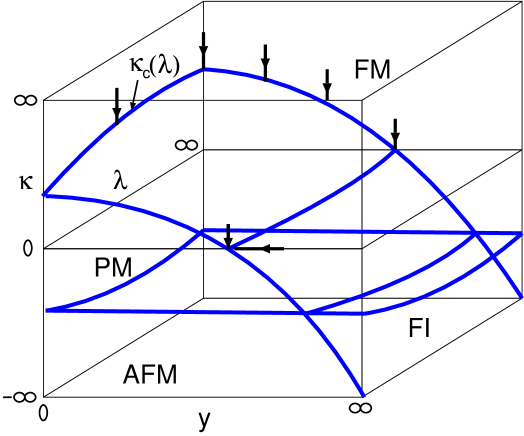
Figure 1: Schematic phase diagram of the Y₃ model. The region below the upper critical surface is the paramagnetic phase (PM), the region above it the ferromagnetic phase (FM). The $y=0$ plane and the $\kappa=\lambda=0$ line correspond to the $\phi_{3}^{4}$ and GN₃ models, respectively. For negative values of the parameter $\kappa$ we further expect an antiferromagnetic phase (AFM) and a ferrimagnetic phase (FI). We have investigated the PM-FM transition for $\kappa\simeq 0$ and $\kappa>0$, in particular at the points and directions indicated by the arrows.

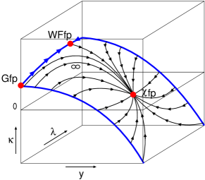
Figure 2: A suggestion for the renormalization group flow on the PM-FM critical surface of the Y₃ model. The fixed points are Gfp (Gaussian), WFfp (Wilson-Fisher) and $\chi$fp (chiral, or GN₃). The indicated position of the $\chi$fp is very schematic, it could lie anywhere on the PM-FM sheet, at $y>0$.

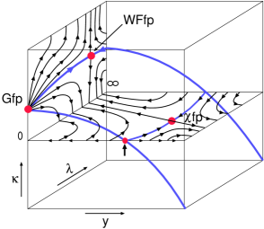
Figure 3: The schematic RG-flow in the $\phi_{3}^{4}$ model ($y=0$, $\kappa>0$), in the $\kappa=0$ surface of the Y₃ model and on the $\kappa=\lambda=0$ line, which corresponds to the GN₃ model. The fixed point of the latter model is indicated by an arrow.

When in the Y₃ model the Yukawa coupling decreases and the $\phi^{4}_{3}$ theory is approached, the WFfp gets presumably influential, as some crossover to the magnetic universality class must occur. This consideration warns us that for limited lattice volumina and consequently limited correlation lengths either no unique finite size scaling behavior can be found or the wrong fixed point dominates. Thus a detection of the genuine – presumably chiral – character of the transition gets more and more difficult in numerical simulations. This is the situation we are most interested in, as it might occur in 4D without a prior warning.

Apart from this particle physics motivation our work might be of interest also for other reasons, related mainly to statistical mechanics:

1. We have applied the Binder method of finite size scaling analysis [14, 15] to the chiral phase transition and found that it works very well also when a composite scalar field is used in the finite size scaling theory, as long as the $\chi$fp alone dominates the finite size scaling behavior.

2. A transition between various universality classes in finite volumina has been investigated recently [16, 17] in some spin models, but, to our knowledge, until now in no models with fermions. Thus we make a new contribution to the experience with this sort of complex finite size behavior. As in spin models, it is the failure of the Binder method which indicates a change of the universality class.

3. Sometimes an intermediate universality class could exist [17]. This would be very surprising for the Y₃ model, nevertheless we have verified that this is most probably not the case here.

We now briefly describe the contents of the paper and the main results:

In the next section we introduce the Y₃ model and determine its phase diagram (fig. 1), both by means of the effective potential in the one loop approximation, and by performing numerical simulations on a small lattice at many points in the three-dimensional parameter space. The most useful order parameter is the scalar field expectation value, even if this field can be considered as composed of a fermion pair. We mention some results on the fermion and boson masses both in the symmetric phase and in the phase with broken chiral symmetry.

In sec. 3 we shortly review the Binder method allowing a determination of several critical exponents by an analysis of finite size effects. The most useful exponent is the correlation length exponent $\nu$ obtained from the Binder-Challa-Landau (BCL) [14, 18] cumulant.

The magnetic transition of the $\phi^{4}_{3}$ theory is investigated in sec. 4. After localizing the critical line we concentrate on the case $\lambda=\infty$ (the XY₃ model) and a case of an intermediate scalar selfcoupling ($\lambda=0.5$). The obtained exponents are consistent with each other and with the value expected from analytic investigations of the WFfp ($\nu=0.67$). Also the values of the renormalized coupling extrapolated to infinite cutoff are consistent. The Binder method is compared with two other approaches to finite size scaling and found to be most suitable for our purposes.

Sec. 5 deals with the chiral transition in the GN₃ model at $\lambda=0$ both in the auxiliary scalar field formulation ($\kappa=0$), and with a dynamical scalar field ($\kappa$ varied and $y$ kept at the critical value, $y=1.09$). In both approaches to the critical point the Binder method works comparably well for all the lattice sizes we used (6³ – 24³) and gives consistent results for critical exponents. In particular, $\nu=1.03(11)$, which is a value consistent with theoretical expectations [13, 19, 20] and significantly different from the value found for the $\phi^{4}_{3}$ model at $y=0$. Thus the difference between the magnetic and chiral universality classes is clearly observed in the $y=0$ and $\lambda=0$ limit cases. Their common property is that the Binder method works in an exemplary way in the whole range of lattice sizes we used.

In sec. 6, the Y₃ model with a large Yukawa coupling, $y=1.1$, is investigated at the maximal value of the scalar selfcoupling $\lambda=\infty$. Also here the Binder method works quite well, and we find $\nu=0.88(6)$, a value slightly lower than, but within errors still consistent with that found in the GN₃ model. This confirms the appurtenance of the Y₃ model with both couplings $y$ and $\lambda$ strong to the same chiral universality class as the GN₃ model, and thus the physical equivalence of both theories.

However, difficulties arise when the Yukawa coupling decreases. As we describe in sec. 7, at $\lambda=\infty$ and $y=0.6$ the BCL cumulants cross at different points when only small (6³ – 10³) or large (10³ – 24³) lattices are considered, suggesting different values of the critical $\kappa$. Restricting ourselves to the larger lattices only, we find the Binder method to work, giving $\nu=0.99(23)$. This value is consistent with the GN₃ model value, but has a large error. On small lattices the obtained value of $\nu$ is significantly lower and close to the value in the $\phi^{4}_{3}$ model. As we describe in detail in the same section, at $\lambda=\infty$ and $y=0.3$ the Binder method gives inconsistent results in the whole range of lattice sizes 6³ – 32³ we have investigated. This can be interpreted as a situation in which none of the two fixed points alone dominates the finite size effects on lattices of these sizes, i.e. as an interplay of or a crossover between universality classes. We find no sign for the existence of an intermediate universality class.

As we conclude in sec. 8, an interplay of magnetic and chiral phenomena in the Y₃ model thus results in uncontrollable finite size effects. However, inconsistencies in the application of finite size methods become apparent only when a broader range of lattice sizes is investigated. This might serve as a warning for investigations of critical points with a mixture of chiral and some other critical behaviour in 4D lattice field theories.

2 The $\mbox{Y}_{3}$ model and its phase diagram

2.1 The action

In order to investigate the breakdown of a continuous chiral symmetry we use staggered fermions [21]. In the lattice parametrization the action of the Y₃ model is

$$S = S_{\mathrm{B}}+S_{\mathrm{F}}+S_{\mathrm{Y}}$$

$$S_{\mathrm{B}} = \sum_{x}\left\{-2\kappa\sum\limits_{\mu}\sum\limits_{i=1}^{2}\phi_{x+\mu}^{i}\phi_{x}^{i}+\sum\limits_{i=1}^{2}\left(\phi_{x}^{i}\right)^{2}+\lambda\left(\sum\limits_{i=1}^{2}(\phi_{x}^{i})^{2}-1\right)^{2}\right\}$$

$$S_{\mathrm{F}} = \frac{1}{2}\sum\limits_{x,\mu}\eta_{x,\mu}\sum\limits_{j=1}^{N_{F}/2}\left(\bar{\chi}_{x}^{j}\chi_{x+\mu}^{j}-\bar{\chi}_{x+\mu}^{j}\chi_{x}^{j}\right)$$

$$S_{\mathrm{Y}} = \frac{y}{2^{3}}\sum\limits_{x,j}\bar{\chi}_{x}^{j}\sum\limits_{b}\left(\phi_{x+b}^{1}+i\varepsilon_{x}\phi_{x+b}^{2}\right)\chi_{x}^{j}\>,$$ (1)

where the integer 3-vectors $x$, $x+\mu$ and $x+b$ denote, respectively, lattice site, its nearest neighbors and corners of the associated elementary cube (both in positive direction). The coefficients are:

$$\eta_{x,1}=1\>,\;\eta_{x,\mu}=(-1)^{x_{1}+\ldots+x_{\mu-1}}\>,\;\varepsilon_{x}=(-1)^{x_{1}+\ldots+x_{3}}\;.$$

The coupling constants $\kappa$, $\lambda$ and $y$ and the fields $\phi^{i}$ and $\chi_{j}$ are dimensionless quantities. $N_{F}=4$ is the number of continuum four-component fermions.

The scalar sector $S_{B}$ of the action (2.1) has a global O(2) symmetry. The action $S$ is invariant under the vectorial U(N) transformations

$$\chi_{j}\rightarrow\Omega_{ji}\chi_{i}\,\,,\,\,\bar{\chi}_{j}\rightarrow\bar{\chi}_{i}\Omega_{ij}^{\dagger}\,\,,\,\,\Omega\in U(N_{F}/2)$$ (2)

and the axial $\mbox{U}(1)_{\mathrm{A}}$ transformations

$$\chi\rightarrow e^{i\omega_{\mathrm{A}}\varepsilon_{x}}\chi\,\,,\,\,\bar{\chi}\rightarrow\bar{\chi}e^{i\omega_{\mathrm{A}}\varepsilon_{x}}\,\,,\,\,\phi\rightarrow e^{-2i\omega_{\mathrm{A}}}\phi\,\,,\,\,\phi^{*}\rightarrow e^{2i\omega_{\mathrm{A}}}\phi^{*}\;,\;\omega_{\mathrm{A}}\in\mbox{l}\!\mbox{R}\;.$$ (3)

The action (2.1) contains two important limit cases, the $\phi_{3}^{4}$ model and the GN₃ model. At $y=0$ it is the $\phi_{3}^{4}$ theory described by the purely scalar part $S_{\mathrm{B}}$ of (2.1). In the limit $\lambda\rightarrow\infty$ the action $S_{B}$ reduces to that of the XY₃ spin model. At $\kappa=\lambda=0$, the action $S$ (2.1) turns into the action of the chiral GN₃ model in the auxiliary scalar field formulation. The full Yukawa model interpolates between both these models and the PM-FM critical sheet continuously connects the magnetic phase transition of the spin model with the chiral phase transition of the GN₃ model.

2.2 Symmetry breaking

In order to get information about the breakdown of the continuous chiral symmetry in the $\mathrm{Y}_{3}$ model we have computed the effective potential in 1-loop order for $\kappa>0$. For this purpose we start with the Euclidean continuum action with $m_{0}$ being the bare mass, $g_{0}$ the bare scalar selfcoupling and $y_{0}$ the bare Yukawa coupling. The calculation is straightforward (see [22]) and yields

$$V_{\mathrm{eff}}(\sigma^{2}) = \frac{m_{0}^{2}}{2}\sigma^{2}+\frac{g_{0}}{4!}(\sigma^{2})^{2}+\frac{1}{2}\int\limits_{\Lambda}\frac{d^{3}p}{(2\pi)^{3}}\,\ln\left(p^{2}+m_{0}^{2}+\frac{g_{0}}{2}\sigma^{2}\right)$$ (4)

$$+ \frac{1}{2}\int\limits_{\Lambda}\frac{d^{3}p}{(2\pi)^{3}}\,\ln\left(p^{2}+m_{0}^{2}+\frac{g_{0}}{6}\sigma^{2}\right)$$

$$- 2N_{F}\int\limits_{\Lambda}\frac{d^{3}p}{(2\pi)^{3}}\ln\left(p^{2}+y_{0}^{2}\sigma^{2}\right)\;,$$

where we have regularized the momentum integrals with a cut-off $\Lambda$. We have introduced the abbreviation $\sigma^{2}=\sigma_{1}^{2}+\sigma_{2}^{2}$, where the constants $\sigma_{i}$ ($i=1,2$) can be identified with the expectation values $\sigma_{i}=\langle\varphi_{i}\rangle$, $\varphi_{i}$ being the scalar fields in the continuum. These fields are related to the lattice scalar fields $\phi_{x}^{i}$ by

$$\varphi_{i}(ax)=\sqrt{\frac{2\kappa}{a}}\phi_{x}^{i}$$ (5)

and the relations between the parameters are

$$m_{0}^{2}=\frac{1-2\lambda-6\kappa}{a^{2}\kappa}~{},~{}~{}g_{0}=\frac{6\lambda}{a\kappa^{2}}~{}.$$ (6)

All the values of $\sigma_{i}$ which minimize $V_{\mathrm{eff}}$ are possible candidates for the vacuum of the theory. We can find these minima by solving the equations $\partial V_{\mathrm{eff}}/\partial\sigma_{i}=0$ simultaneously for $i=1,2$. One solution is $\sigma_{1}=\sigma_{2}=0$. In the symmetric phase it is a minimum ($\partial_{i}\partial_{i}V_{\mathrm{eff}}|_{(0,0)}>0$), in the broken phase a maximum ($\partial_{i}\partial_{i}V_{\mathrm{eff}}|_{(0,0)}<0$) and a further solution exists. In this sense $\partial_{i}\partial_{i}V_{\mathrm{eff}}|_{(0,0)}=0$ is an implicit equation for the boundary between both phases of the theory.

At fixed values of the parameters $m_{0}^{2}$ and $g_{0}$ we can calculate the critical Yukawa coupling $y_{\mathrm{c}}(m_{0}^{2},g_{0})$. If we choose $m_{0}^{2}\geq 0$ we can always find a positive solution $y_{c}$ of $\partial_{i}\partial_{i}V_{\mathrm{eff}}|_{(0,0)}=0$ which is

$$y_{\mathrm{c}}=\left(4N_{F}\int\limits_{\Lambda}\frac{d^{3}p}{(2\pi)^{3}}\,\frac{1}{p^{2}}\right)^{-\frac{1}{2}}\left[m_{0}^{2}+\frac{2}{3}\int\limits_{\Lambda}\frac{d^{3}p}{(2\pi)^{3}}\,\frac{g_{0}}{p^{2}+m_{0}^{2}}\right]^{\frac{1}{2}}\;,\;g_{0}\geq 0\;.$$ (7)

Equation (7) means that even for $m_{0}^{2}\geq 0$, when the classical potential does not predict the symmetry breaking, a solution $y_{\mathrm{c}}(m_{0}^{2},g_{0})$ exists. For all couplings $y_{0}$ with $y_{0}>y_{\mathrm{c}}$ the vacuum expectation value $\langle\varphi\rangle$ of the scalar field is nonzero and the chiral symmetry is broken.

This computation of the 1-loop effective potential suggests that in the $\mathrm{Y}_{3}$ model, at sufficiently small $\kappa\geq 0$, two phases of different symmetry exist, as indicated in fig. 1. As usual, we call them paramagnetic (PM) for $\langle\phi\rangle=0$ and ferromagnetic (FM) for $\langle\phi\rangle\neq 0$.

2.3 The phase diagram

Figure 1 displays a schematic phase diagram, including also some expectations for $\kappa<0$. The phases relevant for our purposes are PM and FM. In the PM phase both order parameters $\langle\phi\rangle$ and $\langle\bar{\chi}\chi\rangle$ (for $y>0$) are zero and fermions are massless. The lightest boson pair is degenerate. In the FM phase the vacuum expectation value of the scalar field, the chiral condensate and fermion mass are nonzero.

To characterize the PM and FM phases numerically we have used the magnetization $M=V^{-1}\sqrt{(\sum_{x}\phi_{x}^{1})^{2}+(\sum_{x}\phi_{x}^{2})^{2}}$, $V$ being the number of lattice points. A continuous phase transition is indicated by a singularity of the susceptibility

$$\chi=V(\langle M^{2}\rangle-\langle M\rangle^{2})\;.$$ (8)

For the numerical simulations we used the Hybrid Monte Carlo algorithm. The critical surface of the phase diagram has been found by localizing peaks of the susceptibility on a $6^{3}$-lattice. In table 1 the values of the coupling parameters at the maxima of the susceptibility are summarized. Of course, they give only an approximate position of the critical surface. In cases in which it was needed, the critical coupling in the thermodynamic limit has been determined by a finite size scaling analysis.

Table 1: Peaks of the susceptibility in the Y₃ model determined on a $6^{3}$ lattice

$y$	$\kappa$	$\lambda$
0	1/6	0
0	0.1730(6)	0.01
0	0.1818(5)	0.03
0	0.2008(10)	0.10
0	0.2265(15)	0.30
0	0.238(2)	0.50
0	0.249(2)	1.00
0	0.240(3)	3.00
0	0.218(2)	$\infty$
1.10(8)	0	0.0
1.25(8)	0	0.5
1.25(10)	0	0.75
1.28(8)	0	1.0
1.25(13)	0	1.5
1.25((13)	0	2.0
1.10(8)	0	$\infty$
0.3	0.15(1)	0
0.6	0.12(1)	0
0.80(8)	0.08	0

$y$	$\kappa$	$\lambda$
0.90(8)	0.05	0
1.42(7)	-0.1	0
0.0	0.24(2)	0.5
0.3	0.22(1)	0.5
0.5	0.20(2)	0.5
0.95(13)	0.1	0.5
1.10(10)	0.6	0.5
1.30(13)	0.0	0.5
0.0	0.25(4)	1.0
0.3	0.22(3)	1.0
1.05(15)	0.06	1.0
1.30(25)	0.0	1.0
0.0	0.22(1)	$\infty$
0.3	0.19(1)	$\infty$
0.6	0.14(1)	$\infty$
0.80(8)	0.1	$\infty$
1.0	0.04(1)	$\infty$
1.10(8)	0.001	$\infty$
1.47(8)	-0.1	$\infty$

Our data strongly supports the expectation that for all positive values of $y$ the condensate $\langle\bar{\chi}\chi\rangle$ vanishes simultaneously with the magnetisation $M$. We have extracted the fermion mass from the fermionic momentum space propagator. The agreement with the tree level prediction $am_{F}=y\langle\phi\rangle$ is quite good. In the FM phase we have also observed in the $\phi$-propagator a massive particle, the $\sigma$-boson, and a massless particle, the Goldstone boson. These masses, as well as $\langle\bar{\chi}\chi\rangle$, are not as convenient as the BCL cumulant for the study of the finite size behavior but can be used for a qualitative comparison of the physical content of the Y₃ model in different parameter regions.

2.4 Renormalizability properties

Both the $\phi^{4}$ theory and the full Yukawa model in 3D are perturbatively superrenormalizable. For the GN₃ model this is different. The continuum 4-fermion coupling has negative mass dimension, and the corresponding interaction is therefore perturbatively nonrenormalizable. Nevertheless, it has been proved that the GN₃ model is renormalizable in the $1/N_{F}$-expansion [23].

It has also been shown in the framework of $1/N_{F}$-expansion that for weak scalar selfcoupling $\lambda=O(1/N_{F})$ the Gross-Neveu model and the full Yukawa model in $2<d<4$ are equivalent field theories [9, 10, 11]. Near the nontrivial fixed point the kinetic term of the scalar field and the quartic scalar selfinteraction turn out to be irrelevant operators. However, in those works nothing beyond the range of validity of the $1/N_{F}$-expansion could be said.

In ref. [12] the equivalence has been confirmed by analytic and numerical methods for the discrete chiral Z(2)-symmetry, still with $\lambda=O(1/N_{F})$. We have extended that work to the U(1)-symmetric case and have investigated a wide range of parameters including infinite scalar selfcoupling.

3 Finite size scaling theory

3.1 The Binder method

In order to examine the interplay of the universality classes associated with two different nontrivial fixed points in the Y₃ model we have studied the finite size scaling behavior and tried to determine the critical exponents of the theory at several points of the critical surface. A very powerful method to do this is the Binder method of finite size scaling analysis of a cumulant [14, 15].

It is sufficient to use scalar n-point functions even in the case of nonvanishing Yukawa coupling. We therefore follow refs. [15, 24] and define the corresponding fourth-order cumulant $U_{L}$ on a cubic lattice of extent $L$:

$$U_{L}=-\frac{\frac{1}{V}\tilde{G}_{L}^{(4)}-2\left[\tilde{G}_{L}^{(2)}\right]^{2}}{\left[\tilde{G}_{L}^{(2)}\right]^{2}}\;,\;V=L^{3}\;,$$ (9)

where $\tilde{G}_{L}^{(2)}$ and $\tilde{G}_{L}^{(4)}$ are

$$\tilde{G}_{L}^{(2)} = \frac{1}{V}\sum\limits_{x_{1},x_{2}}\sum\limits_{i}\langle\phi_{x_{1}}^{i}\phi_{x_{2}}^{i}\rangle$$

$$\tilde{G}_{L}^{(4)} = \frac{1}{V}\sum\limits_{x_{1},\ldots,x_{4}}\sum\limits_{i,j}\langle\phi_{x_{1}}^{i}\phi_{x_{2}}^{i}\phi_{x_{3}}^{j}\phi_{x_{4}}^{j}\rangle\;.$$ (10)

If both $L$ and the correlation length $\xi$ are sufficiently large then $U_{L}$ has the form

$$U_{L}=2-\frac{f_{4}\left(\frac{L}{\xi}\right)}{\left[f_{2}\left(\frac{L}{\xi}\right)\right]^{2}}\;$$ (11)

with analytic functions $f_{2}$ and $f_{4}$. Note that (11) requires the validity of hyperscaling.

At the critical value $\kappa_{c}$ of the hopping parameter $\kappa$ the correlation length diverges and all cumulants $U_{L}|_{\kappa_{\mathrm{c}}}$ have the same value $U^{*}$ independent of the lattice size. This makes it possible to determine the infinite volume critical coupling as the common intersection point of $U_{L}$ for different values of $L$.

In the scaling limit Binder’s cumulant has the form

$$U_{L}(t)=U\left(\frac{L}{\xi(t)}\right)=\tilde{U}(tL^{\frac{1}{\nu}})\;\;,\;\;|t|\ll 1$$ (12)

with $t=1-\kappa_{\mathrm{c}}/\kappa$. Let us consider a pair $(bL,L)$ of lattice sizes with $b>1$. From (12) it follows

$$\ln\left(\frac{\partial U_{bL}}{\partial U_{L}}\bigg{|}_{\kappa_{\mathrm{c}}}\right)=\frac{1}{\nu}\ln b\;.$$ (13)

In order to obtain the derivative $\frac{\partial U_{bL}}{\partial U_{L}}|_{\kappa_{\mathrm{c}}}$ one calculates the function $U_{bL}=g(U_{L})$ numerically and near the critical point approximates $g$ by a linear function determining its slope.

Similar relations can easily be derived for the exponent $\gamma$ of the susceptibility $\chi$ and the exponent $\beta$ of the magnetisation $M$,

$$\ln\left(\frac{\chi_{bL}(\kappa_{\mathrm{c}})}{\chi_{L}(\kappa_{\mathrm{c}})}\right) = \frac{\gamma}{\nu}\ln b$$

$$\ln\left(\frac{M_{bL}(\kappa_{\mathrm{c}})}{M_{L}(\kappa_{\mathrm{c}})}\right) = -\frac{\beta}{\nu}\ln b\;.$$ (14)

Using (3.1) one can calculate the ratios $\beta/\nu$ and $\gamma/\nu$ from $M$ and $\chi$ determined on various lattice sizes $(bL,L)$ exactly at $\kappa_{\mathrm{c}}$.

In the $\phi_{3}^{4}$ theory the specific heat exponent $\alpha$ is negative. That means that the specific heat is a regular function of the reduced coupling and there is no relation similar to (3.1) for it.

To calculate the required quantities, we used a reweighting technique. By means of the original method due to Ferrenberg and Swendsen [25] one can only interpolate operators which can be expressed as explicite functions of $S$. Therefore, like the authors of ref. [12], we used a variation of the method suggested in ref. [26]. It can be regarded as the multihistogram method with bins of zero width. With that reweighting technique one can interpolate nearly arbitrary operators over a wide range of the coupling $\beta$. For this purpose it is necessary to store the operator $S$ which corresponds to the coupling $\beta$ and the value of the operator for each configuration which has been generated during the simulation.

3.2 Previous applications of the Binder method

In the past the Binder method has been applied to a variety of interesting physical systems. In ref. [24] the method has been generalized to $O(N)$ $\phi^{4}$ theories and in ref. [27] the critical exponent $\nu$ has been determined for the $\mathrm{O}(4)$ invariant scalar $\phi^{4}$ theory in 3D and 4D. A high precision measurement of $\nu$ in the XY₃ model has been done in ref. [28].

The method has also been applied to models with interacting fermions [12]. Here a slight modification of the Binder method has been used to compute the critical exponents $\nu$ and $\gamma/\nu$ in the 3-dimensional Gross-Neveu model with Z(2)-symmetry. The found value of $\nu\approx 1$ is in good agreement with the prediction of the $1/N_{F}$-expansion.

In ref. [17] the critical behaviour of diluted Heisenberg ferromagnets with competing interactions has been investigated. The authors varied the concentration of spins and found two distinct universality classes which are separated by a crossover region. In this domain strong corrections to scaling appear, and Binder’s method does not work well. Also evidence for a new, intermediate universality class has been found.

3.3 Other methods to determine critical exponents

For the $\phi_{3}^{4}$ model we have also tried to compute critical indices by some other methods. Among these are the direct method, which makes use of the finite size scaling laws of physical quantities, and the scaling of the smallest Lee-Yang zero with the lattice size.

On a finite lattice of extent $L$ the susceptibility peaks at the value $\kappa_{M}(L)$ of the hopping parameter. If we increase the lattice size then $\kappa_{M}(L)$ approaches $\kappa_{c}$ according to

$$\kappa_{M}(L)-\kappa_{c}~{}\propto~{}L^{-1/\nu}.$$ (15)

Thus the measurement of $\kappa_{M}(L)$ for various lattice sizes $L$ yields the critical exponent $\nu$ by a corresponding fit. We have tried this method in the $\phi_{3}^{4}$ theory for different values of the scalar selfcoupling $\lambda$. Our results were rather unsatisfactory because of their quite large statistical errors. For the same statistics we obtained more accurate values for $\nu$ with the Binder method.

Another possibility to determine $\nu$ is to use the finite size scaling of the Lee-Yang-Fisher zeroes. By continuing the hopping parameter $\kappa$ to complex values one finds that the partition function has zeroes in the complex plain. For finite lattices all the zeroes lie off the real axis. The zero $\kappa_{0}$ with the smallest imaginary part scales like [29]

$$\mathrm{Im}(\kappa_{0})\sim L^{-\frac{1}{\nu}}\;.$$

We have computed $\mathrm{Im}(\kappa_{0})$ on different lattices and extracted $\nu$ from a double logarithmic plot. Our results are consistent with those obtained by the other methods but the statistical errors again turned out to be substantially larger than for the Binder method.

4 Magnetic transition at vanishing Yukawa coupling

4.1 The $\phi_{3}^{4}$ model

In the limit $y=0$ the action (2.1) describes free massless fermions and $O(2)$ invariant $\phi_{3}^{4}$ model with quartic selfcoupling. Besides our interest in the features of the $\phi_{3}^{4}$ model as a limit of the Yukawa theory, here we have developed and tested the methods we wanted to apply to the more sophisticated and expensive fermionic model. The existence of a nontrivial fixed point and a finite nonvanishing value of the renormalized quartic selfcoupling $\lambda_{R}$ in the continuum limit make this model by itself very interesting from a field theoretic point of view, too.

The phase diagram in the $\kappa$-$\lambda$ plane, computed mainly on $6^{3}$ lattices (see the $y=0$ entries in the table 1), is displayed in fig. 4. The spectrum in the PM phase below the second order phase transition line contains two degenerate massive scalar particles. In the FM phase ($\kappa>\kappa_{c}$) the $O(2)$ symmetry is spontaneously broken and the lightest particles in the spectrum are a massless Goldstone boson and a massive $\sigma$ boson.

Figure 4: Phase diagramm of the $\phi_{3}^{4}$ model. The $\lambda$-axis has been rescaled: $\lambda^{*}=50\lambda/(1+5\lambda)$. The circles show the maxima of the susceptibility on a $6^{3}$ lattice. The crosses show the positions of $\kappa_{c}$ determined with higher precision by means of finite size scaling methods.

The renormalization group properties of the $\phi_{3}^{4}$ model have been investigated e.g. in [30] and are indicated in figs. 2 and 3 on the $y=0$ face of the phase diagram at $\kappa>0$. The model is superrenormalizable in weak coupling perturbation theory and its physics at infinitesimal scalar selfcoupling is dominated by the Gaussian fixed point (Gfp) at $\lambda=0$. At nonvanishing coupling $\lambda>0$ the critical line $\kappa_{c}(\lambda)$ is dominated by the IR-stable nontrivial WFfp. The investigations by means of $\varepsilon$ expansion or $1/N$ expansion of the $O(N)$ symmetric $\phi_{3}^{4}$ suggest that the interaction term becomes irrelevant, and the only relevant term remains the kinetic one. This means that at $\lambda>0$ only one parameter has to be tuned $\kappa\rightarrow\kappa_{c}(\lambda)$ in order to reach a continuum limit governed by the WFfp. Thus the same scaling behavior should be found when the critical line is approached at arbitrary $\lambda>0$.

4.2 Results at ${\mathbf{\lambda}=\infty}$ and ${\mathbf{\lambda}=0.5}$

We have chosen $\lambda=\infty$ and $\lambda=0.5$ and determined the renormalized coupling as well as some critical indices in runs in the $\kappa$ direction. A Monte Carlo determination of the renormalized quartic coupling $\lambda_{R}$ has been done e.g. in [31] for the $Z(2)$ symmetric $\phi_{3}^{4}$ model. To our knowledge no analogous measurement exists for the $O(2)$ symmetric model. Following e.g. [31] we define $\lambda_{R}$ in the symmetric phase as

$$\lambda_{R}=(Lam_{R})^{3}U_{L}~{}.$$ (16)

Here $am_{R}$ is the mass of the $\sigma$-boson extracted from the scalar propagator. To extrapolate to the continuum limit we varied the lattice size from $L=6$ to $12$ while keeping $Lam_{R}$ fixed to $4$.

At $\lambda=\infty$ the renormalized scalar selfcoupling increases very slowly with the lattice size $L$. The linear extrapolation in $1/L$ to $L=\infty$ suggests a value of $\lambda_{R}=26\pm 4$. At $\lambda=0.5$ an extrapolation to $L=\infty$ is less precise, suggesting $\lambda_{R}=20-30$. The agreement supports the expectation, that the model is dominated by the WFfp on the whole critical line $\lambda>0$. These results for $\lambda_{R}$ are also consistent with the expected theoretical value [32].

The most sensitive test for the appurtenance to the same universality class is the comparison of critical exponents. Using the Binder method described in subsec. 3.1 we have determined the critical exponents $\nu$, $\beta/\nu$ and $\gamma/\nu$. The method works very well at both $\lambda$ values in the whole range of lattice sizes used, $4^{3}-16^{3}$. To illustrate this we show in fig. 5 the determination of $\kappa_{c}$ at $\lambda=0.5$. In fig. 6 the data for $\partial U_{bL}/\partial U_{L}$, used for the determination of $\nu$ at the same $\lambda$ value, and the linear fit, are displayed.

Figure 5: The intersection point of the Binder cumulants in the $\phi^{4}_{3}$ model on several lattices for $\lambda=0.5$ at $\kappa_{c}=0.241(1)$. The lines were obtained by reweighting, the symbols are the measured points.

Figure 6: Linear fit to $\ln(\partial U_{bL}/\partial U_{L})$ used, according to eq. 13, for the determination of the critical exponent $\nu$ determined at $\lambda=0.5$.

$\lambda$	$\kappa_{c}$	$\nu$	$\beta/\nu$	$\gamma/\nu$	$(\alpha)$	$(\delta)$	$(\eta)$
$\infty$	0.2275(10)	0.673(19)	0.51(3)	2.03(6)	-0.02(6)	5.2(4)	0.02(6)
0.5	0.241(1)	0.687(19)	0.56(5)	1.91(6)	-0.06(6)	4.5(3)	0.12(10)

Table 2: Critical exponents in the $\phi_{3}^{4}$ model at $\lambda=0.5$ and $\lambda=\infty$. The exponents enclosed in brackets were calculated by using hyperscaling relations.

We were able to determine $\nu$ to a precision of about $3\%$, $\beta/\nu$ to about $9\%$ and $\gamma/\nu$ to $3\%$. The results are summarized in table 2. They are consistent with the expectation that the two points $\lambda=\infty$ and $\lambda=0.5$ belong to the same universality class. The value of $\beta/\nu$ is consistent with the one calculated with the hyperscaling relation $\beta/\nu=(d-\gamma/\nu)/2$. As hyperscaling seems to be fulfilled, we determined the exponents $\alpha$, $\delta$ and $\eta$ from the relations

$$\alpha=2-\nu d,\quad\delta=\frac{d+\gamma/\nu}{d-\gamma/\nu},\quad\eta=2-d+2\frac{\beta}{\nu}~{}.$$

5 Chiral transition at vanishing scalar selfcoupling

5.1 The GN₃ model

At $\lambda=\kappa=0$ the scalar field $\phi$ plays in the action (2.1) the role of an auxiliary field. It can be integrated out thus obtaining a purely fermionic GN₃ model with U(1) chiral symmetry,

$$S=S_{F}-\frac{y^{2}}{4}\left[\left(\frac{1}{8}\sum\limits_{b\in h.c.}\overline{\chi}_{x+b}\chi_{x+b}\right)^{2}-\left(\frac{1}{8}\sum\limits_{b\in h.c.}\epsilon_{x+b}\overline{\chi}_{x+b}\chi_{x+b}\right)^{2}\right].$$ (17)

In 3D this model is perturbatively non-renormalizable. However, it has been shown in [33, 8] that the GN₃ model is renormalizable in the $1/N_{F}$ expansion. The $\beta$-function has been calculated to $O(1/N_{F})$ in [13, 19] and to $O(1/N_{F}^{2})$ in [20]. The $1/N_{F}$ expansion reveals a nontrivial UV-stable fixed point where dynamical chiral symmetry breaking and fermion mass generation occur. The phase transition is of $2^{\rm nd}$ order and the order parameter is the chiral condensate $\langle\overline{\chi}\chi\rangle$.

In ref. [20] one can find the critical exponent $\nu$ to $O(1/N_{F}^{2})$. In our case ($N_{F}=4$)

$$\nu=1+\frac{16}{3\pi^{2}N_{F}}-\frac{8(376+27\pi^{2})}{27\pi^{4}N_{F}^{2}}+O(1/N_{F}^{3})\simeq 1+0.135-0.122\simeq 1.0(1)~{}.$$ (18)

The $O(1/N_{F})$ term is identical with the results in [19, 13]. The $O(1/N_{F}^{2})$ term is of the same order of magnitude, which suggests a rather large error on the value of $\nu$ in (18).

In the symmetric phase ($y<y_{c}$) fermions are massless. This region is dominated by the trivial Gaussian fixed point at $y=0$.

By adding the kinetic scalar term to the bare GN₃ action the scalar field $\phi$ turns from an auxiliary field to a dynamical one. This restricted Yukawa model with $\lambda=0$, sometimes considered as a sufficient representation of the $Y_{3}$ model (e.g. in [11]), is a natural extension of the parameter space of the GN₃ model. We know that such a Yukawa model with vanishing scalar selfcoupling and $Z(2)$ symmetry is renormalizable in $1/N_{F}$ expansion. As shown in [9, 10], this model has a nontrivial IR-stable fixed point where the kinetic term of the scalar field becomes irrelevant and the 4-fermion interaction term relevant. This fixed point is identical with the critical GN₃ model. The IR-stable fixed point of this restricted Yukawa model corresponds to the UV-stable fixed point of the GN₃ model [9, 10, 11]. This can be understood from the renormalization group flow in a larger parameter space, in the full Y₃ model (2.1) (see figure 3). The flow is suggested by the $\beta$-functions obtained in the $\epsilon$-expansion [9]. The RG-flow restricted to the GN₃-line $\kappa=\lambda=0$ is consistent with the UV-stability of the nontrivial GN₃ fixed point.

5.2 Numerical results

First we comment on the spectrum calculations. The fermion mass $am_{F}$ has been measured by fitting the momentum space fermion propagator, measured usually at four lattice momenta, to a free fermion ansatz. In the broken phase $am_{F}$ agrees very well with the tree level relation $am_{F}=y\langle\phi\rangle=\frac{y^{2}}{2}\langle\overline{\chi}\chi\rangle$.

For the measurement of the masses of the $\sigma$-boson $am_{\sigma}$ and the Goldstone boson $am_{\pi}$ we had to use an ansatz for the momentum space propagators from the one-loop renormalized perturbation theory [34]. In this case the previously fitted fermion mass is used to calculate the fermionic selfenergy which contributes to the renormalized bosonic propagators. This method delivers the renormalized Yukawa coupling and describes very well the form of the bosonic propagators which differ very much from the free ones. As expected, in the FM phase $am_{\pi}$ is very small and $am_{\sigma}$ increases with the distance from the critical point. In the PM phase both masses grow with the distance from the critical point and become degenerate.

The scaling behavior has been investigated in two directions: In the GN₃ case ($\kappa=0$) we varied $y$ and determined the critical Yukawa coupling $y_{c}=1.091(5)$ from the intersection point of the Binder cumulants on several lattices. From the finite size scaling behavior of the Binder cumulant at this value we determined the exponent $\nu$. Similarly the behavior of magnetization and susceptibility allowed us to determine $\beta/\nu$ and $\gamma/\nu$, respectively. The obtained results are collected in table 3.

$\kappa_{c}$	$y_{c}$	$\nu$	$\beta/\nu$	$\gamma/\nu$	note
0	1.091(5)	1.02(8)	0.89(10)	1.19(13)	run in $y$ (GN)
0.000(2)	1.09	1.05(12)	0.90(4)	1.15(4)	run in $\kappa$

Table 3: The critical exponents $\nu$, $\beta/\nu$, $\gamma/\nu$ in the GN₃ model and in the Yukawa model at vanishing $\lambda$.

By using the measured $\gamma/\nu$ value one obtains from the hyperscaling relations $\beta/\nu=0.905(65)$. This is in good agreement with the measured value and supports the hyperscaling hypothesis.

As a test of our methods and of the equivalence between the fixed points of the GN₃ and the Yukawa model with vanishing $\lambda$ we measured the critical exponents in the latter model by approaching the critical point of the GN₃ model along the $\kappa$ direction. Fig. 7 demonstrates that the critical point obtained by the Binder method in this direction is identical with the GN₃ one. The BCL cumulants intersect at $\kappa_{c}=0.000(2)$ and $y_{c}=1.09$. As shown in fig. 8, the values of $\beta/\nu$ and $\gamma/\nu$ are perfectly consistent with those obtained in the GN₃ run (table 3).

Figure 7: Determination of $\kappa_{c}$ in the Yukawa model at $\lambda=0$ and $y=1.09$. The intersection point of the BCL cumulants measured on different lattice sizes gives $\kappa_{c}=0.000(2)$ which is in perfect agreement with the GN₃ critical point.

Figure 8: Determination of the critical exponent $\nu$ in the Yukawa model at $\lambda=0$, $y=1.09$ and $\kappa=0$.

We conclude that the Binder finite size scaling method is applicable and gives consistent results in the Yukawa model at $\lambda=0$ for a broad range of lattice sizes. The values of the critical exponents in the chiral GN₃ model are the same as in the Yukawa model with $\lambda=0$. This confirms that the fixed points of these two models are the same. The exponents are consistent with the $1/N_{F}$ predicted values ($\nu\approx 1$) and significantly different from the exponents associated with the WFfp. This allows us to investigate the crossover effects between these universality classes numerically.

6 Gross-Neveu-like behaviour for strong couplings

The $1/N$ expansion predicts [9, 10, 11] that the Y₃ model and the GN₃ models are equivalent at least for weak scalar selfcoupling $\lambda$. In order to test this hypothesis also for strong scalar couplings we have investigated the Y₃ model with $\lambda=\infty$ at strong bare Yukawa coupling $y=1.1$. This choice leads to $\kappa_{c}\simeq 0$.

The spectrum is similar to that of the GN₃ model. We observe the generation of the fermion mass $am_{F}$ which is related to a nonzero chiral condensate $\langle\overline{\chi}\chi\rangle$. Even for $\lambda=\infty$, where the $1/N_{F}$-expansion is not applicable, we find that the prediction $am_{F}\approx y\langle\phi\rangle$ is fulfilled with good precision. Fig. 9 displays the dependence of the masses of both bosons on the hopping parameter $\kappa$ at $y=1.1$ and $\lambda=\infty$. In accordance with the Goldstone theorem one massive $\sigma$ boson and one massless $\pi$ boson appear in the FM phase. The qualitative $\kappa$-dependence of both masses in the vicinity of the critical point is the same as in the Y₃ model at $\lambda=0$. This is a first numerical hint for the physical equivalence of both cases.

Figure 9: The masses of the $\sigma$- and $\pi$-bosons as functions of $\kappa$. As expected, in the broken phase the $\sigma$ boson is massive and the $\pi$ boson massless.

In order to determine the universality class of the Y₃ model at $\lambda=\infty$ and strong Yukawa coupling we have again determined the critical exponents $\nu$, $\beta/\nu$ and $\gamma/\nu$. We have applied the Binder method at $y=1.1$ approaching the critical sheet in the $\kappa$ direction. The critical value $\kappa_{\mathrm{c}}=0.007(2)$ is given by the common intersection point of the cumulants $U_{L}$ on different lattices sizes $L$.

For this value of $\kappa_{\mathrm{c}}$ we have computed the derivatives $\partial U_{bL}/\partial U_{L}$ with $L=6$ and $bL$ ranging from 8 to 24. Figure 10 shows as an example $U_{bL}$ as a function of $U_{L}$ for $b=4$. Near the critical point such functions are linear with good precision and the derivatives are thus easily determined.

Figure 10: An example ($L=6$, $b=4$) of the linear dependence of $U_{bL}$ on $U_{L}$ at $\lambda=\infty$, $y=1.1$ near the critical point.

Using equation (13) we have obtained the critical exponent $\nu$,

$$\nu=0.89(6)\;.$$ (19)

This value is a little bit smaller than the one obtained at $\lambda=0$, but both values are consistent within statistical errors. Figure 11 shows the corresponding plot. We have also made various fits with different subsets of data points. The results are nearly unaffected if we leave out one or more data points in the fit. This shows that also for $\lambda=\infty$ and $y=1.1$ corrections to scaling are quite small and the Binder method works in a broad range of lattice sizes.

Figure 11: Log-log plot of the derivative $\partial U_{bL}/\partial U_{L}$ at $\kappa_{\mathrm{c}}$ at $\lambda=\infty$, $y=1.1$. We show the linear fits to the first three,$\dots$, six points. The results of these fits are consistent values $\nu_{3},\ldots,\nu_{6}$ of the exponent $\nu$.

We have further determined the ratios $\beta/\nu$ and $\gamma/\nu$,

$$\frac{\beta}{\nu} = 0.80(8),$$

$$\frac{\gamma}{\nu} = 1.30(7)\;.$$ (20)

Within statistical errors these exponents are consistent with our results in the GN₃ model, too. They fulfill the corresponding hyperscaling relation with good precision.

These numerical results lead us to the conclusion that the Gross-Neveu universality class extends over the whole range from $\lambda=0$ to $\lambda=\infty$ provided the bare Yukawa coupling $y$ is strong enough, $y\simeq 1$. This confirms the conjecture that the GN₃ model and the $\mathrm{Y}_{3}$ model are equivalent field theories even for $\lambda=\infty$.

7 Interplay of magnetic and chiral universality classes

Both in the pure scalar $\phi^{4}_{3}$ theory at $y=0$ and in the GN₃ model at $\lambda=0$ the Binder method works in an exemplary way. Also in the Y₃ model at $\lambda=\infty$, $y=1.1$ it provides satisfactory results. This is presumably due to the dominance of only one of the fixed points in these cases. They seem to be “pure” cases, without any interplay of universality classes. Now we describe what happens in the Y₃ model when at $\lambda=\infty$ the Yukawa coupling $y$ is decreased, and the XY₃ model is approached. We made extensive simulations at $y=0.6$ and $y=0.3$, approaching the critical sheet in the $\kappa$ direction.

7.1 ${\mathbf{\lambda}=\infty}$, ${\mathbf{y}=0.6}$

For small lattice sizes, $L=6,8,10$, the cumulants consistently cross in the interval $\kappa=0.1460-0.1466$ (fig. 12a). Making the finite size analysis at $\kappa=0.1463$ we obtain $\nu=0.75(9)$, a value quite close to that of the XY₃ model.

Figure 12: Determination of $\kappa_{c}$ at $\lambda=\infty$ and $y=0.6$. On small lattices (a) the apparent critical $\kappa$ is 0.1463, but including also data on larger lattices and zooming into the rectangular region (b) suggests that the critical point is in the interval $\kappa=0.1435-0.1445$ of the intersection points of $U_{L}$ for $L\geq 10$.

However, when only large lattices $L=10,12,14,16,24$ are considered, the crossing point is found in the interval $\kappa=0.1430-0.1445$. The situation is shown on a fine $\kappa$ scale in fig. 12b. For these lattices at $\kappa=0.144$ we find $\nu=0.99(23)$, a value consistent with the GN₃ model, but with a large error.

Figure 13: Similar to fig. 11, but now at $\lambda=\infty$, $y=0.6$. The $\nu$-values increase systematically when data on larger and larger lattices is included in the linear fit.

We have made an analysis at $\kappa_{c}=0.144$ including data on all lattices and choosing the basis $L=6$. The $\nu$ values have been determined for different groups of data, for the first 3, 4, 5 and 6 points. As shown in fig. 13, when data on larger and larger lattices is included, $\nu$ increases systematically from 0.71(11) for $b=8/6$, 10/6 and 12/6 only, to 0.87(8) when all data is included. This is probably not a good way of analysis in such a complex situation and the previous one made only on large lattices seems to be more reliable. We have made it in order to illustrate the systematic increase of the apparent $\nu$ with lattice size.

We interpret the above results as a hint that for sufficiently large lattices, $L\geq 10$, the $\chi$fp universality class finally shows up. It might be tempting to conjecture that the low value of $\nu$, obtained rather consistently for $L\leq 10$, is a signal for the nearby WFfp class. But, as the results at $y=0.3$ indicate, this is questionable.

Figure 14: An attempt to determine $\kappa_{c}$ at $\lambda=\infty$, $y=0.3$ failed. $U_{L}$ do not intersect in a single point even if only large lattices are considered.

Figure 15: Example ($L=6$, $b=4$) of nonlinear dependence of $U_{bL}$ on $U_{L}$ at $\lambda=\infty$, $y=0.3$ near the critical point.

7.2 ${\mathbf{\lambda}=\infty}$, ${\mathbf{y}=0.3}$

As seen in fig. 14, the cumulants obtained on lattices up to $L=32$ show no tendency to cross at some unique point, even if smaller lattices are discarded. Also the dependence of $U_{\rm bL}$ on $U_{\rm L}$, shown in fig. 15, is not linear, differing e.g. from $\lambda=\infty,y=1.1$, seen in fig. 10. A determination of $\nu$ under these circumstances makes little sense, and one can only speculate that if lattices could be made still substantially larger, a simpler finite size behavior with the $\chi$fp exponents might be found.

Remarkable is also the fact that the finite size behavior did not improve on small lattices. As in the $y=0.6$ case, the cumulants on $L\leq 10$ lattices cross in a narrow interval $\kappa_{c}=0.2045-0.2055$. But including the $L=12$ data spoils the consistency completely. Thus halving the distance from the XY₃ model with respect to $y=0.6$ did not increase the consistency of the finite size behaviour for smaller lattice sizes. This prevents us from interpreting the low values of $\nu$ obtained on smaller lattices as a signal for the WFfp universality class.

Attempts to incorporate some corrections to the leading finite size behaviour, as suggested in ref. [27], are in our case not very helpful because simulations with dynamical fermions cannot yet produce data with the precision needed to deal with additional parameters. Thus, we conclude that at $\lambda=\infty$ and $y=0.3$ the finite size behaviour is not under control. Unfortunately, it would not have been easy to notice that without having data in a large range of lattice sizes.

8 Summary and Conclusions

We have studied the finite size behavior of the Y₃ model with U(1) chiral symmetry along the 2 dimensional sheet of chiral phase transitions at various values of the Yukawa coupling $y$ and of the scalar selfcoupling $\lambda$. The aim was to investigate the influence and the interplay of the two nongaussian fixed points of the model for various values of the couplings.

In the $y=0$ limit case, i.e. in the $\phi^{4}_{3}$ model, the critical exponents associated with the Wilson-Fisher fixed point (WFfp) are clearly observed both at $\lambda=\infty$ and $\lambda=0.5$. The Binder method of finite size scaling analysis is applicable already on small lattices. Also the renormalized coupling values agree and are consistent with the theoretical prediction. The WFfp thus provides a rather complete description of the model at least for $\lambda\geq 0.5$.

For $y>0$ we find that the chiral fixed point ($\chi$fp) determines the finite size scaling in the vicinity of the chiral phase transition sheet as long as the Yukawa coupling is strong enough, $y\simeq 1$. The independence on the value of the quartic coupling $\lambda$ confirms the expectation that the $Y_{3}$ model and its special case, the GN₃ model, belong to the same universality class of the $\chi$fp. Also the fermion and boson masses at $\lambda=0$ and $\lambda=\infty$ are very similar. For $y\simeq 1$ the Binder method of finite size scaling analysis works consistently in a broad range of lattice sizes, in analogy to the pure $\phi_{3}^{4}$ theory. No substantial difference in the finite size behavior has been found between $\lambda=0$ and $\lambda=\infty$. This implies that as long as $y$ is large enough, the $\lambda\phi^{4}$ term does not influence the finite size behavior of the Y₃ model even on small lattices and the model is rather completely described by the $\chi$fp.

When, at $\lambda=\infty$, $y$ is decreased to $y=0.6$, the finite size behavior cannot be analysed any more by the Binder method in the whole range of the lattice sizes we used. The behavior on small ($L\leq 10$) and large ($L\geq 10$) lattices is different. On the larger lattices the $\chi$fp seems still to dominate. On the smaller lattices the behavior looks consistent with the WFfp. But this does not necessarily mean that the WFfp already starts to show up: when a further step towards the $\phi^{4}_{3}$ limit case is made, at $\lambda=\infty$ and $y=0.3$, the finite size behavior does not show increased resemblance to that fixed point. If applied in a narrow interval of lattice sizes, the Binder method might seem to be applicable but the results are misleading.

A numerical verification of the expectation that the Y₃ model is equivalent to the GN₃ model is thus very difficult for $y\leq 0.6$. Our tentative conclusion is that the observed deviation from the simple finite size scaling signals an interplay of both universality classes, i.e. a crossover between them. This warns us that in the situation of intertwining phenomena the finite size behavior may be very complex. As we learned in the $\lambda=\infty,y=0.6$ case, this fact is not easily detectable in a small range of lattice sizes, however.

References

-
[1]
Recent references are e.g.:
S.J. Hands, A. Kocić, J.B. Kogut, R.L. Renken, D.K. Sinclair and K.C. Wang, Nucl. Phys. B413 (1994) 503.
M. Göckeler, R. Horsley, P. Rakow, G. Schierholz and R. Sommer, Nucl. Phys. B371 (1992) 713.
V. Azcoiti, G. Di Carlo, A. Galante, A.F. Grillo, V. Laliena and C.E. Piedrafita, Phys. Lett. B353 (1995) 279. -
[2]
For a recent investigation of the critical behavior
in pure QED see:
J. Jersák, C.B. Lang and T. Neuhaus, Nucl. Phys. B (Proc. Suppl.) 42 (1995) 672. - [3] M. Okawa, Phys. Rev. Lett. 62 (1989) 1224.
-
[4]
Recent references are e.g.:
K.-I. Kondo, A. Shibata, M. Tanabashi and K. Yamawaki, Progr. Theor. Phys. 91 (1994) 541.
M. Harada, Y. Kikukawa, T. Kugo and H. Nakano, Progr. Theor. Phys. 92 (1994) 1161.
V. Azcoiti, G. Di Carlo, A. Galante, A.F. Grillo, V. Laliena and C.E. Piedrafita, Phys. Lett. B355 (1995) 270. -
[5]
Recent references are:
C. Frick and J. Jersák, Phys. Rev. D52 (1995) 340;
W. Franzki, C. Frick, J. Jersák and X.Q. Luo, Nucl. Phys. B453 (1995) 355. - [6] A. Ali Khan, M. Göckeler, R. Horsley, P. Rakow, G. Schierholz and H. Stüben, Phys. Rev. D51 (1995) 3751.
- [7] K.G. Wilson and M.E. Fisher, Phys. Rev. Lett. 28 (1972) 240.
- [8] B. Rosenstein, B.J. Warr and S. Park, Phys. Rep. 205 (1991) 59.
- [9] J. Zinn-Justin, Nucl. Phys. B367 (1991) 105.
- [10] A. Kovner and B. Rosenstein, Phys. Lett. B261 (1991) 97.
- [11] G. Gat, A. Kovner and B. Rosenstein, Nucl. Phys. B385 (1992) 76.
- [12] L. Kärkkäinen, R. Lacaze, P. Lacock and B. Petersson, Nucl. Phys. B415 (1994) 781; Erratum ibid. B438 (1995) 650.
- [13] S. Hands, A. Kocić and J.B. Kogut, Ann. Phys. 224 (1993) 29.
- [14] K. Binder, Z. Physik B43 (1981) 119.
- [15] K. Binder, “Finite Size Effects at Phase Transitions”, in H. Gausterer and C.B. Lang (eds.), “Computational Methods in Field Theory”, Springer, Berlin (1992), p. 59.
- [16] K. Binder and H.-P. Deutsch, Europhys. Lett. 18 (1992) 667.
-
[17]
M. D’Onorio DeMeo, J.D. Reger and K. Binder,
Physica A (1995) (in print);
in Computer Simulation Studies in Condensed Matter Physics VI, eds. D.P. Landau et. al., Springer Berlin (1993), p. 193. - [18] K. Binder, M.S.S. Challa and D.P. Landau, Phys. Rev. B34 (1986) 1841.
- [19] H.J. He, Y.P. Kuang, Q. Wang and Y.P. Yi, Phys. Rev. D45 (1992) 4610.
- [20] J.A. Gracey, Phys. Rev. D50 (1994) 2840.
- [21] L. Susskind, Phys. Rev. D16 (1977) 3031.
- [22] C. Itzykson and J.-B. Zuber, “Quantum Field Theory”, McGraw–Hill (1980).
- [23] S.H. Park, B. Rosenstein and B.J. Warr, Phys. Rep. 205 (1991) 59.
- [24] W. Bernreuther and M. Göckeler, Nucl. Phys. B295 [FS21] (1988) 199.
- [25] A.M. Ferrenberg and R.H. Swendsen, Phys. Rev. Lett. 63 (1989) 1195.
- [26] K. Kajantie, L. Kärkkäinen and K. Rummukainen, Nucl. Phys. B357 (1991) 693.
- [27] W. Bernreuther, M. Göckeler and M. Kremer, Nucl. Phys. B295 [FS21] (1988) 211.
- [28] W. Janke, Phys. Lett. A148 (1990) 306.
- [29] C. Itzykson, R.B. Pearson and J.B. Zuber, Nucl. Phys. B220 [FS8] (1983) 415.
- [30] E. Brezin, G.C. Le Guillou and J. Zinn-Justin, Phys. Rev. D8 (1973) 2418.
- [31] B. Freedman, P. Smolensky and D. Weingarten, Phys. Lett. 113B (1982) 481.
- [32] J. Zinn-Justin, “Quantum field theory and critical phenomena”, Oxford University Press, 1989.
- [33] B. Rosenstein, B.J. Warr and S. Park, Phys. Rev. Lett. 62 (1989) 1433.
-
[34]
W. Bock, A.K. De, C. Frick, J. Jersák and
T. Trappenberg, Nucl. Phys. B378 (1992) 652.
C. Frick, PhD thesis at RWTH Aachen, 1993.